Massively parallel semi-Lagrangian solutionof the 6d Vlasov-Poisson problem

Katharina Kormann1 Klaus Reuter2

Markus Rampp2 Eric Sonnendrucker1

1Max–Planck–Institut fur Plasmaphysik

2Max Planck Computing and Data Facility

October 20, 2016

Introduction

Interpolation und Parallelization

Numerical comparison of interpolators

Code optimization

Overlap of computation and communication

1

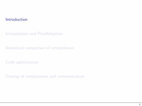
Vlasov–Poisson equation and characteristics

Vlasov–Poisson equation for electrons in neutralizing background

∂f (t, x, v)

∂t+ v · ∇xf (t, x, v)− E(t, x) · ∇vf (t, x, v) = 0,

−∆φ(t, x) = 1− ρ(t, x), E(t, x) = −∇φ(t, x),

ρ(t, x) =

∫f (t, x, v) dv.

Advection equation keeps values along characteristics:

dX

dt= V,

dV

dt= −E(t,X).

Solution: f (t, x, v) = f0(X(0; t, x, v),V(0; t, x, v))

2

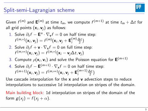
Split-semi-Lagrangian scheme

Given f (m) and E(m) at time tm, we compute f (m+1) at time tm + ∆t forall grid points (xi , vj) as follows:

1. Solve ∂t f − En · ∇vf = 0 on half time step:

f (m,∗)(xi , vj) = f (m)(xi , vj + E(m)i

∆t2 )

2. Solve ∂t f + v · ∇xf = 0 on full time step:f (m,∗∗)(xi , vj) = f (m,∗)(xi − vj∆t, vj)

3. Compute ρ(xi , vi ) and solve the Poisson equation for E(m+1)

4. Solve ∂t f − E(m+1) · ∇xf = 0 on half time step:

f (m+1)(xi , vj) = f (m,∗∗)(xi , vj + E(m+1)i

∆t2 )

Use cascade interpolation for the x and v advection steps to reduceinterpolations to successive 1d interpolation on stripes of the domain.

Main building block: 1d interpolation on stripes of the domain of theform g(xj) = f (xj + α).

3

Introduction

Interpolation und Parallelization

Numerical comparison of interpolators

Code optimization

Overlap of computation and communication

4

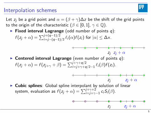
Interpolation schemes

Let zj be a grid point and α = (β + γ)∆z be the shift of the grid pointsto the origin of the characteristic (β ∈ [0, 1], γ ∈ Q).

I Fixed interval Lagrange (odd number of points q):

f (zj + α) =∑j+(q−1)/2

i=j−(q−1)/2 `i (α)f (zi ) for |α| ≤ ∆x .

r r r r rzj zj + α

I Centered interval Lagrange (even number of points q):

f (zj + α) = f (zj+γ + β) =∑j+γ+q/2

i=j+γ+q/2−1 `i (β)f (zi ).

r r r rzj zj + α

I Cubic splines: Global spline interpolant by solution of linearsystem, evaluation as f (zj + α) =

∑j+γ+2i=j+γ−1 ciSi (β).

r r r rzj zj + α

c c c c c c c5

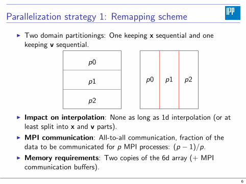
Parallelization strategy 1: Remapping scheme

I Two domain partitionings: One keeping x sequential and onekeeping v sequential.

p0

p1

p2

p0 p1 p2

I Impact on interpolation: None as long as 1d interpolation (or atleast split into x and v parts).

I MPI communication: All-to-all communication, fraction of thedata to be communicated for p MPI processes: (p − 1)/p.

I Memory requirements: Two copies of the 6d array (+ MPIcommunication buffers).

6

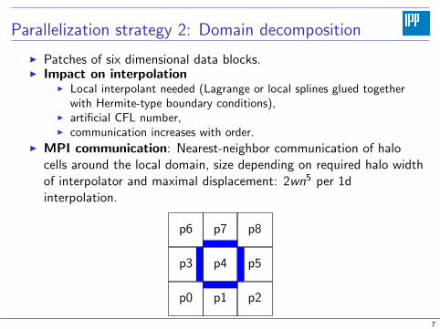
Parallelization strategy 2: Domain decomposition

I Patches of six dimensional data blocks.I Impact on interpolation

I Local interpolant needed (Lagrange or local splines glued togetherwith Hermite-type boundary conditions),

I artificial CFL number,I communication increases with order.

I MPI communication: Nearest-neighbor communication of halocells around the local domain, size depending on required halo widthof interpolator and maximal displacement: 2wn5 per 1dinterpolation.

p0 p1 p2

p3 p4 p5

p6 p7 p8

7

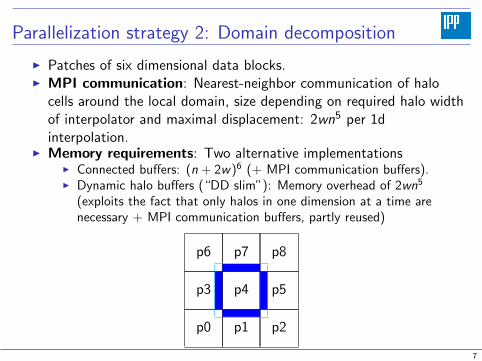
Parallelization strategy 2: Domain decomposition

I Patches of six dimensional data blocks.I MPI communication: Nearest-neighbor communication of halo

cells around the local domain, size depending on required halo widthof interpolator and maximal displacement: 2wn5 per 1dinterpolation.

I Memory requirements: Two alternative implementationsI Connected buffers: (n + 2w)6 (+ MPI communication buffers).I Dynamic halo buffers (“DD slim”): Memory overhead of 2wn5

(exploits the fact that only halos in one dimension at a time arenecessary + MPI communication buffers, partly reused)

p0 p1 p2

p3 p4 p5

p6 p7 p8

7

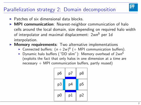
Parallelization strategy 2: Domain decomposition

I Patches of six dimensional data blocks.I MPI communication: Nearest-neighbor communication of halo

cells around the local domain, size depending on required halo widthof interpolator and maximal displacement: 2wn5 per 1dinterpolation.

I Memory requirements: Two alternative implementationsI Connected buffers: (n + 2w)6 (+ MPI communication buffers).I Dynamic halo buffers (“DD slim”): Memory overhead of 2wn5

(exploits the fact that only halos in one dimension at a time arenecessary + MPI communication buffers, partly reused)

p0 p1 p2

p3 p4 p5

p6 p7 p8

7

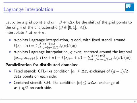
Lagrange interpolation

Let xi be a grid point and α = β + γ∆x be the shift of the grid points tothe origin of the characteristic (β ∈ [0, 1], γQ).Interpolate f at xi + α.

I q-points Lagrange interpolation, q odd, with fixed stencil around:

f (xj + α) =∑j+(q−1)/2

i=j−(q−1)/2 `i (α)f (xi )

I q-points Lagrange interpolation, q even, centered around the interval

[xi+γ , xi+γ+1]: f (xj + α) = f (xj+γ + β) =∑j+γ+q/2

i=j+γ+q/2−1 `i (β)f (xi )

Parallelization for distributed domains:

I Fixed stencil: CFL-like condition |α| ≤ ∆z , exchange of (q − 1)/2data points on each side.

I Centered stencil: CFL-like condition |α| ≤ w∆z , exchange ofw + q/2 on each side.

8

Impact of domain decomposition

I Imposes a CFL-like condition.

I Vlasov–Poisson: CFL-like condition is dominated by x-advectionsbut here α = ∆tv constant over time.

I Idea: Use the knowledge of sign of α to reduce data transfer.Resulting data transfer for CFL-like condition α = (w + β)∆z forcentered stencil: max(q/2−w , 0) on left side, q/2 +w on right side.Total data to be sent: q if w ≤ q/2.

9

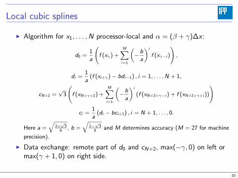
Local cubic splines

I Computation of interpolant: Use local spline on each domain withHermite-type boundary conditions from neighboring domains1.

I Use fast algorithm introduced by Unser et al.2.I Algorithm for x1, . . . ,N processor-local and α = (β + γ)∆x :

d0 =1

a

(f (xγ) +

M∑i=1

(−b

a

)i

f (xγ−i )

),

di =1

a(f (xi+γ)− bdi−1) , i = 1, . . . ,N + 1,

cN+2 =√

3

(f (xN+γ+2) +

M∑i=1

(−b

a

)i

(f (xN+2+γ−i ) + f (xN+2+γ+i ))

)

ci =1

a(di − bci+1) , i = N + 1, . . . , 0.

Here a =√

2+√

36

, b =√

2−√

36

and M determines accuracy (M = 27 for machine

precision).1Crouseilles et al., J. Comput. Phys. 228, 20092Unser et al., IEEE Trans. Pattern Anal. Mach. Intell. 13, 1991

10

Local cubic splines

I Algorithm for x1, . . . ,N processor-local and α = (β + γ)∆x :

d0 =1

a

(f (xγ) +

M∑i=1

(−b

a

)i

f (xγ−i )

),

di =1

a(f (xi+γ)− bdi−1) , i = 1, . . . ,N + 1,

cN+2 =√

3

(f (xN+γ+2) +

M∑i=1

(−b

a

)i

(f (xN+2+γ−i ) + f (xN+2+γ+i ))

)

ci =1

a(di − bci+1) , i = N + 1, . . . , 0.

Here a =√

2+√

36

, b =√

2−√

36

and M determines accuracy (M = 27 for machine

precision).

I Data exchange: remote part of d0 and cN+2, max(−γ, 0) on left ormax(γ + 1, 0) on right side.

10

Introduction

Interpolation und Parallelization

Numerical comparison of interpolators

Code optimization

Overlap of computation and communication

11

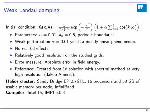
Weak Landau damping

Initial condition: f0(x, v) = 1(2π)3/2 exp

(− |v|

2

2

)(1 + α

∑3`=1 cos(k`x`)

)I Parameters: α = 0.01, kx = 0.5, periodic boundaries.

I Weak perturbation α = 0.01 yields a mostly linear phenomenon.

I No real 6d effects.

I Relatively good resolution on the studied grids.

I Error measure: Absolute error in field energy.

I Reference: Created from 1d solution with spectral method at veryhigh resolution (Jakob Ameres).

Helios cluster: Sandy-Bridge EP 2.7GHz, 16 processors and 58 GB ofusable memory per node, InfiniBandCompiler: Intel 15, IMPI 5.0.3

12

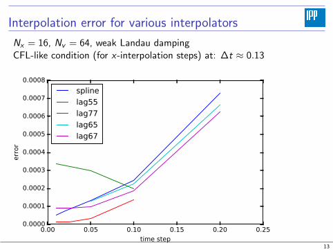
Interpolation error for various interpolators

Nx = 16, Nv = 64, weak Landau dampingCFL-like condition (for x-interpolation steps) at: ∆t ≈ 0.13

0.00 0.05 0.10 0.15 0.20 0.25time step

0.0000

0.0001

0.0002

0.0003

0.0004

0.0005

0.0006

0.0007

0.0008

error

splinelag55lag77lag65lag67

13

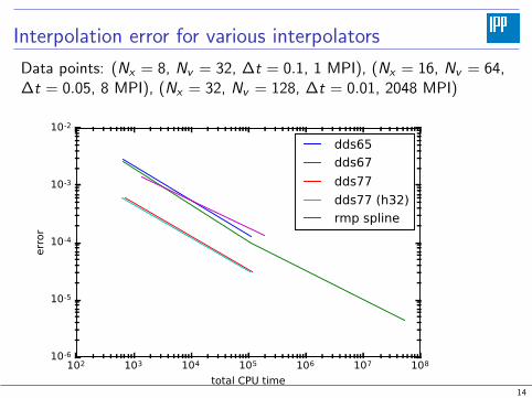
Interpolation error for various interpolators

Data points: (Nx = 8, Nv = 32, ∆t = 0.1, 1 MPI), (Nx = 16, Nv = 64,∆t = 0.05, 8 MPI), (Nx = 32, Nv = 128, ∆t = 0.01, 2048 MPI)

102 103 104 105 106 107 108

total CPU time

10-6

10-5

10-4

10-3

10-2

error

dds65dds67dds77dds77 (h32)rmp spline

14

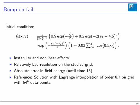
Bump-on-tail

Initial condition:

f0(x, v) = 1(2π)3/2

(0.9 exp(− v2

12 ) + 0.2 exp(−2(v1 − 4.5)2

)exp

(− (v2

2 +v23 )2

2

)(1 + 0.03

∑3`=1 cos(0.3x`)

).

I Instability and nonlinear effects.

I Relatively bad resolution on the studied grid.

I Absolute error in field energy (until time 15).

I Reference: Solution with Lagrange interpolation of order 6,7 on gridwith 646 data points.

15

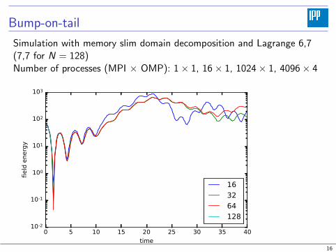
Bump-on-tail

Simulation with memory slim domain decomposition and Lagrange 6,7(7,7 for N = 128)Number of processes (MPI × OMP): 1× 1, 16× 1, 1024× 1, 4096× 4

0 5 10 15 20 25 30 35 40time

10-2

10-1

100

101

102

103

field ene

rgy

163264128

16

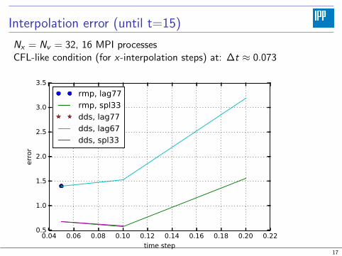
Interpolation error (until t=15)

Nx = Nv = 32, 16 MPI processesCFL-like condition (for x-interpolation steps) at: ∆t ≈ 0.073

0.04 0.06 0.08 0.10 0.12 0.14 0.16 0.18 0.20 0.22

time step

0.5

1.0

1.5

2.0

2.5

3.0

3.5

error

rmp, lag77

rmp, spl33

dds, lag77

dds, lag67

dds, spl33

17

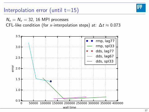
Interpolation error (until t=15)

Nx = Nv = 32, 16 MPI processesCFL-like condition (for x-interpolation steps) at: ∆t ≈ 0.073

0 50000 100000 150000 200000 250000 300000 350000 400000

wall time

0.5

1.0

1.5

2.0

2.5

3.0

3.5

error

rmp, lag77

rmp, spl33

dds, lag77

dds, lag67

dds, spl33

17

Introduction

Interpolation und Parallelization

Numerical comparison of interpolators

Code optimization

Overlap of computation and communication

18

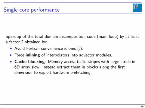
Single core performance

Speedup of the total domain decomposition code (main loop) by at leasta factor 2 obtained by:

I Avoid Fortran convenience idioms (:).

I Force inlining of interpolators into advector modules.

I Cache blocking: Memory access to 1d stripes with large stride in6D array slow. Instead extract them in blocks along the firstdimension to exploit hardware prefetching.

19

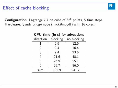
Effect of cache blocking

Configuration: Lagrange 7,7 on cube of 326 points, 5 time steps.Hardware: Sandy bridge node (mick@mpcdf) with 16 cores.

CPU time (in s) for advectionsdirection blocking no blocking

1 5.9 12.62 9.4 16.43 9.4 23.54 21.6 48.15 26.9 55.16 29.7 86.0

sum 102.9 241.7

20

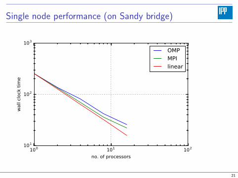
Single node performance (on Sandy bridge)

100 101 102

no. of processors

101

102

103

wall clock

tim

e

OMP

MPI

linear

21

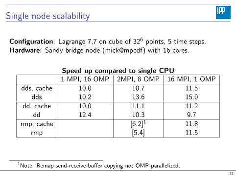
Single node scalability

Configuration: Lagrange 7,7 on cube of 326 points, 5 time steps.Hardware: Sandy bridge node (mick@mpcdf) with 16 cores.

Speed up compared to single CPU1 MPI, 16 OMP 2MPI, 8 OMP 16 MPI, 1 OMP

dds, cache 10.0 10.7 11.5dds 10.2 13.6 15.0

dd, cache 10.0 11.1 11.2dd 12.4 10.3 9.7

rmp, cache [6.2]1 11.8rmp [5.4] 11.5

1Note: Remap send-receive-buffer copying not OMP-parallelized.22

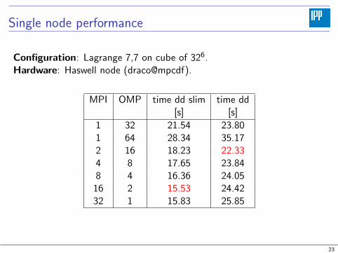
Single node performance

Configuration: Lagrange 7,7 on cube of 326.Hardware: Haswell node (draco@mpcdf).

MPI OMP time dd slim time dd[s] [s]

1 32 21.54 23.801 64 28.34 35.172 16 18.23 22.334 8 17.65 23.848 4 16.36 24.05

16 2 15.53 24.4232 1 15.83 25.85

23

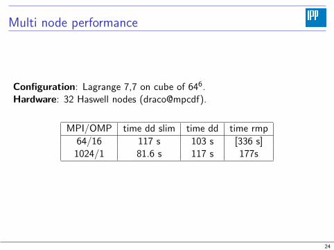
Multi node performance

Configuration: Lagrange 7,7 on cube of 646.Hardware: 32 Haswell nodes (draco@mpcdf).

MPI/OMP time dd slim time dd time rmp

64/16 117 s 103 s [336 s]1024/1 81.6 s 117 s 177s

24

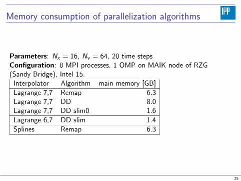
Memory consumption of parallelization algorithms

Parameters: Nx = 16, Nv = 64, 20 time stepsConfiguration: 8 MPI processes, 1 OMP on MAIK node of RZG(Sandy-Bridge), Intel 15.

Interpolator Algorithm main memory [GB]

Lagrange 7,7 Remap 6.3Lagrange 7,7 DD 8.0Lagrange 7,7 DD slim0 1.6

Lagrange 6,7 DD slim 1.4

Splines Remap 6.3

25

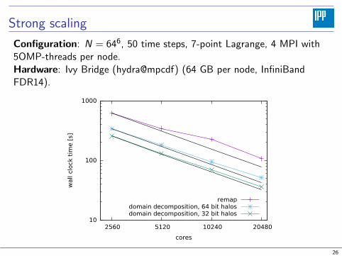
Strong scaling

Configuration: N = 646, 50 time steps, 7-point Lagrange, 4 MPI with5OMP-threads per node.Hardware: Ivy Bridge (hydra@mpcdf) (64 GB per node, InfiniBandFDR14).

10

100

1000

2560 5120 10240 20480

wall

clock

tim

e [

s]

cores

remapdomain decomposition, 64 bit halosdomain decomposition, 32 bit halos

26

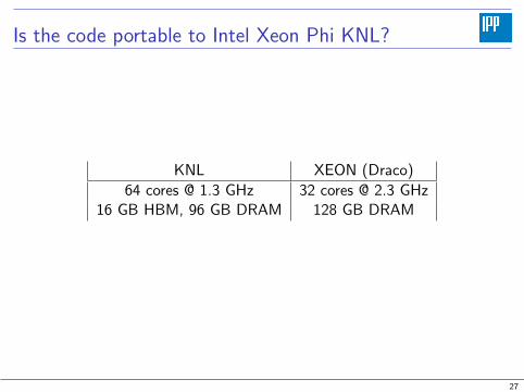
Is the code portable to Intel Xeon Phi KNL?

KNL XEON (Draco)

64 cores @ 1.3 GHz 32 cores @ 2.3 GHz16 GB HBM, 96 GB DRAM 128 GB DRAM

27

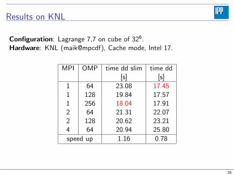
Results on KNL

Configuration: Lagrange 7,7 on cube of 326.Hardware: KNL (maik@mpcdf), Cache mode, Intel 17.

MPI OMP time dd slim time dd[s] [s]

1 64 23.08 17.451 128 19.84 17.571 256 18.04 17.912 64 21.31 22.072 128 20.62 23.214 64 20.94 25.80

speed up 1.16 0.78

28

Results on KNL

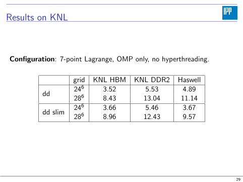
Configuration: 7-point Lagrange, OMP only, no hyperthreading.

grid KNL HBM KNL DDR2 Haswell

dd246 3.52 5.53 4.89286 8.43 13.04 11.14

dd slim246 3.66 5.46 3.67286 8.96 12.43 9.57

29

Introduction

Interpolation und Parallelization

Numerical comparison of interpolators

Code optimization

Overlap of computation and communication

30

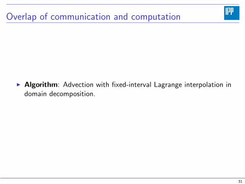
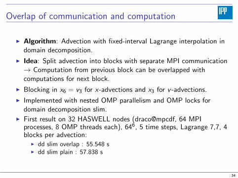
Overlap of communication and computation

I Algorithm: Advection with fixed-interval Lagrange interpolation indomain decomposition.

31

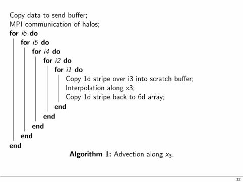
Copy data to send buffer;MPI communication of halos;for i6 do

for i5 dofor i4 do

for i2 dofor i1 do

Copy 1d stripe over i3 into scratch buffer;Interpolation along x3;Copy 1d stripe back to 6d array;

end

end

end

end

endAlgorithm 1: Advection along x3.

32

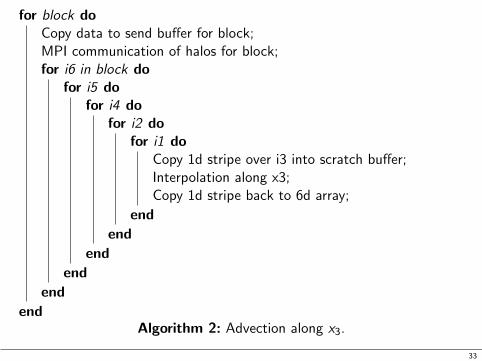
for block doCopy data to send buffer for block;MPI communication of halos for block;for i6 in block do

for i5 dofor i4 do

for i2 dofor i1 do

Copy 1d stripe over i3 into scratch buffer;Interpolation along x3;Copy 1d stripe back to 6d array;

end

end

end

end

end

endAlgorithm 2: Advection along x3.

33

Overlap of communication and computation

I Algorithm: Advection with fixed-interval Lagrange interpolation indomain decomposition.

I Idea: Split advection into blocks with separate MPI communication→ Computation from previous block can be overlapped withcomputations for next block.

I Blocking in x6 = v3 for x-advections and x3 for v -advections.

I Implemented with nested OMP parallelism and OMP locks fordomain decomposition slim.

I First result on 32 HASWELL nodes (draco@mpcdf, 64 MPIprocesses, 8 OMP threads each), 646, 5 time steps, Lagrange 7,7, 4blocks per advection:

I dd slim overlap : 55.548 sI dd slim plain : 57.838 s

34

Overlap: Preliminary results

0

1

2

0 10 20 30 40 50 60 70

thre

ad

id

time [s]

adv prep exch

I Note: Advection (adv) and halo preparation (prep) use nestedOpenMP threads to utilize all available CPU cores

35

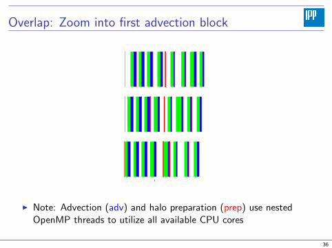
Overlap: Zoom into first advection block

I Note: Advection (adv) and halo preparation (prep) use nestedOpenMP threads to utilize all available CPU cores

36

Conclusions

Summary

I Interpolation: Lagrange better than splines for good resolution,splines for low resolution. Lagrange better suited for distributeddomains.

I Memory-slim implementation of domain decomposition enablessolution of large-scale problems.

I Domain decomposition scales better than remap on thousands ofprocessors.

I Remap algorithm gives more flexibility on time step size and forglobal interpolants.

Outlook

I Include magnetic field and multidimensional interpolation.

I Further exploit the potential of overlapping communication andcomputation.

37