Markov processes - uni-bonn.de · PDF file4.3.2 CLT for Markov processes ... A stochastic...
253
Markov processes Andreas Eberle March 15, 2015
Transcript of Markov processes - uni-bonn.de · PDF file4.3.2 CLT for Markov processes ... A stochastic...

Markov processes
Andreas Eberle
March 15, 2015
Contents
Contents 2
0 Introduction 6
0.1 Stochastic processes . . . . . . . . . . . . . . . . . . . . . . . . . . . . .. . . . 6
0.2 Transition functions and Markov processes . . . . . . . . . . .. . . . . . . . . 7
0.3 Generators and Martingales . . . . . . . . . . . . . . . . . . . . . . . .. . . . . 12
0.4 Stability and asymptotic stationarity . . . . . . . . . . . . . .. . . . . . . . . . 14
1 Markov chains & stochastic stability 16
1.1 Transition probabilities and Markov chains . . . . . . . . . .. . . . . . . . . . 16
1.1.1 Markov chains . . . . . . . . . . . . . . . . . . . . . . . . . . . . . . . 17
1.1.2 Markov chains with absorption . . . . . . . . . . . . . . . . . . . .. . . 19
1.2 Generators and martingales . . . . . . . . . . . . . . . . . . . . . . . .. . . . . 20
1.2.1 Generator . . . . . . . . . . . . . . . . . . . . . . . . . . . . . . . . . . 21
1.2.2 Martingale problem . . . . . . . . . . . . . . . . . . . . . . . . . . . . .21
1.2.3 Potential theory for Markov chains . . . . . . . . . . . . . . . .. . . . . 23
1.3 Lyapunov functions and recurrence . . . . . . . . . . . . . . . . . .. . . . . . . 29
1.3.1 Recurrence of sets . . . . . . . . . . . . . . . . . . . . . . . . . . . . . 30
1.3.2 Global recurrence . . . . . . . . . . . . . . . . . . . . . . . . . . . . . .35
1.4 The space of probability measures . . . . . . . . . . . . . . . . . . .. . . . . . 40
1.4.1 Weak topology . . . . . . . . . . . . . . . . . . . . . . . . . . . . . . . 40
1.4.2 Prokhorov’s theorem . . . . . . . . . . . . . . . . . . . . . . . . . . . .42
1.4.3 Existence of invariant probability measures . . . . . . .. . . . . . . . . 44
1.5 Couplings and transportation metrics . . . . . . . . . . . . . . . .. . . . . . . . 46
1.5.1 Wasserstein distances . . . . . . . . . . . . . . . . . . . . . . . . . .. . 46
1.5.2 Kantorovich-Rubinstein duality . . . . . . . . . . . . . . . . . .. . . . 51
1.5.3 Contraction coefficients . . . . . . . . . . . . . . . . . . . . . . . . .. 52
2
CONTENTS 3
1.5.4 Glauber dynamics, Gibbs sampler . . . . . . . . . . . . . . . . . .. . . 55
1.6 Geometric and subgeometric convergence to equilibrium. . . . . . . . . . . . . 61
1.6.1 Total variation norm . . . . . . . . . . . . . . . . . . . . . . . . . . . .61
1.6.2 Geometric ergodicity . . . . . . . . . . . . . . . . . . . . . . . . . . .. 63
1.6.3 Couplings of Markov chains and convergence rates . . . . .. . . . . . . 67
1.7 Mixing times . . . . . . . . . . . . . . . . . . . . . . . . . . . . . . . . . . . . 72
1.7.1 Upper bounds in terms of contraction coefficients . . . .. . . . . . . . . 73
1.7.2 Upper bounds by Coupling . . . . . . . . . . . . . . . . . . . . . . . . . 74
1.7.3 Conductance lower bounds . . . . . . . . . . . . . . . . . . . . . . . . .75
2 Ergodic averages 77
2.1 Ergodic theorems . . . . . . . . . . . . . . . . . . . . . . . . . . . . . . . . .. 78
2.1.1 Ergodicity . . . . . . . . . . . . . . . . . . . . . . . . . . . . . . . . . . 78
2.1.2 Ergodicity of stationary Markov chains . . . . . . . . . . . .. . . . . . 80
2.1.3 Birkhoff’s ergodic theorem . . . . . . . . . . . . . . . . . . . . . . .. . 82
2.1.4 Application to Markov chains . . . . . . . . . . . . . . . . . . . . .. . 87
2.2 Ergodic theory in continuous time . . . . . . . . . . . . . . . . . . .. . . . . . 89
2.2.1 Ergodic theorem . . . . . . . . . . . . . . . . . . . . . . . . . . . . . . 89
2.2.2 Applications . . . . . . . . . . . . . . . . . . . . . . . . . . . . . . . . 92
2.2.3 Ergodic theory for Markov processes . . . . . . . . . . . . . . .. . . . 97
2.3 Structure of invariant measures . . . . . . . . . . . . . . . . . . . .. . . . . . . 100
2.3.1 The convex set ofΘ-invariant probability measures . . . . . . . . . . . . 100
2.3.2 The set of stationary distributions of a transition semigroup . . . . . . . . 102
2.4 Quantitative bounds & CLT for ergodic averages . . . . . . . . .. . . . . . . . 103
2.4.1 Bias and variance of stationary ergodic averages . . . . .. . . . . . . . 103
2.4.2 Central limit theorem for Markov chains . . . . . . . . . . . . .. . . . . 106
2.4.3 Central limit theorem for martingales . . . . . . . . . . . . . .. . . . . 109
2.5 Asymptotic stationarity & MCMC integral estimation . . . .. . . . . . . . . . . 110
2.5.1 Asymptotic bounds for ergodic averages . . . . . . . . . . . .. . . . . . 112
2.5.2 Non-asymptotic bounds for ergodic averages . . . . . . . .. . . . . . . 114
3 Continuous time Markov processes, generators and martingales 117
3.1 Jump processes and diffusions . . . . . . . . . . . . . . . . . . . . . .. . . . . 118
3.1.1 Jump processes with finite jump intensity . . . . . . . . . . .. . . . . . 118
3.1.2 Markov property . . . . . . . . . . . . . . . . . . . . . . . . . . . . . . 123
University of Bonn Winter term 2014/2015
4 CONTENTS
3.1.3 Generator and backward equation . . . . . . . . . . . . . . . . . .. . . 127
3.1.4 Forward equation and martingale problem . . . . . . . . . . .. . . . . . 130
3.1.5 Diffusion processes . . . . . . . . . . . . . . . . . . . . . . . . . . . .. 135
3.2 Lyapunov functions and stability . . . . . . . . . . . . . . . . . . .. . . . . . . 136
3.2.1 Non-explosion criteria . . . . . . . . . . . . . . . . . . . . . . . . .. . 137
3.2.2 Hitting times and recurrence . . . . . . . . . . . . . . . . . . . . .. . . 140
3.2.3 Occupation times and existence of stationary distributions . . . . . . . . 141
3.3 Semigroups, generators and resolvents . . . . . . . . . . . . . .. . . . . . . . . 143
3.3.1 Sub-Markovian semigroups and resolvents . . . . . . . . . .. . . . . . 143
3.3.2 Strong continuity and Generator . . . . . . . . . . . . . . . . . .. . . . 146
3.3.3 Strong continuity of transition semigroups of Markovprocesses . . . . . 148
3.3.4 One-to-one correspondence . . . . . . . . . . . . . . . . . . . . . .. . 151
3.3.5 Hille-Yosida-Theorem . . . . . . . . . . . . . . . . . . . . . . . . . .. 154
3.4 Martingale problems for Markov processes . . . . . . . . . . . .. . . . . . . . 155
3.4.1 From Martingale problem to Generator . . . . . . . . . . . . . .. . . . 156
3.4.2 Identification of the generator . . . . . . . . . . . . . . . . . . .. . . . 157
3.4.3 Uniqueness of martingale problems . . . . . . . . . . . . . . . .. . . . 161
3.4.4 Strong Markov property . . . . . . . . . . . . . . . . . . . . . . . . . .163
3.5 Feller processes and their generators . . . . . . . . . . . . . . .. . . . . . . . . 165
3.5.1 Existence of Feller processes . . . . . . . . . . . . . . . . . . . .. . . . 165
3.5.2 Generators of Feller semigroups . . . . . . . . . . . . . . . . . .. . . . 168
3.6 Limits of martingale problems . . . . . . . . . . . . . . . . . . . . . .. . . . . 172
3.6.1 Weak convergence of stochastic processes . . . . . . . . . .. . . . . . . 172
3.6.2 From Random Walks to Brownian motion . . . . . . . . . . . . . . . . .175
3.6.3 Regularity and tightness for solutions of martingale problems . . . . . . 178
3.6.4 Construction of diffusion processes . . . . . . . . . . . . . . .. . . . . 182
3.6.5 The general case . . . . . . . . . . . . . . . . . . . . . . . . . . . . . . 184
4 Convergence to equilibrium 186
4.1 Stationary distributions and reversibility . . . . . . . . .. . . . . . . . . . . . . 189
4.1.1 Stationary distributions . . . . . . . . . . . . . . . . . . . . . . .. . . . 189
4.1.2 Reversibility . . . . . . . . . . . . . . . . . . . . . . . . . . . . . . . . 193
4.1.3 Application to diffusions inRn . . . . . . . . . . . . . . . . . . . . . . . 195
4.2 Poincaré inequalities and convergence to equilibrium .. . . . . . . . . . . . . . 197
4.2.1 Decay of variances and correlations . . . . . . . . . . . . . . .. . . . . 198
Markov processes Andreas Eberle
CONTENTS 5
4.2.2 Divergences . . . . . . . . . . . . . . . . . . . . . . . . . . . . . . . . . 202
4.2.3 Decay ofχ2 divergence . . . . . . . . . . . . . . . . . . . . . . . . . . . 205
4.3 Central Limit theorem for Markov processes . . . . . . . . . . . .. . . . . . . . 208
4.3.1 CLT for continuous-time martingales . . . . . . . . . . . . . . .. . . . 210
4.3.2 CLT for Markov processes . . . . . . . . . . . . . . . . . . . . . . . . . 210
4.4 Logarithmic Sobolev inequalities and entropy bouds . . .. . . . . . . . . . . . . 212
4.4.1 Logarithmic Sobolev inequalities and hypercontractivity . . . . . . . . . 212
4.4.2 Decay of relative entropy . . . . . . . . . . . . . . . . . . . . . . . .. . 214
4.4.3 LSI on product spaces . . . . . . . . . . . . . . . . . . . . . . . . . . . 217
4.4.4 LSI for log-concave probability measures . . . . . . . . . .. . . . . . . 220
4.4.5 Stability under bounded perturbations . . . . . . . . . . . .. . . . . . . 225
4.5 Concentration of measure . . . . . . . . . . . . . . . . . . . . . . . . . . .. . . 227
A Appendix 230
A.1 Conditional expectation . . . . . . . . . . . . . . . . . . . . . . . . . . .. . . . 230
A.2 Martingales . . . . . . . . . . . . . . . . . . . . . . . . . . . . . . . . . . . . .231
A.2.1 Filtrations . . . . . . . . . . . . . . . . . . . . . . . . . . . . . . . . . . 232
A.2.2 Martingales and supermartingales . . . . . . . . . . . . . . . .. . . . . 232
A.2.3 Doob Decomposition . . . . . . . . . . . . . . . . . . . . . . . . . . . . 233
A.3 Gambling strategies and stopping times . . . . . . . . . . . . . .. . . . . . . . 235
A.3.1 Martingale transforms . . . . . . . . . . . . . . . . . . . . . . . . . .. 235
A.3.2 Stopped Martingales . . . . . . . . . . . . . . . . . . . . . . . . . . . .237
A.3.3 Optional Stopping Theorems . . . . . . . . . . . . . . . . . . . . . .. . 241
A.4 Almost sure convergence of supermartingales . . . . . . . . .. . . . . . . . . . 242
A.4.1 Doob’s upcrossing inequality . . . . . . . . . . . . . . . . . . . .. . . . 243
A.4.2 Proof of Doob’s Convergence Theorem . . . . . . . . . . . . . . . .. . 245
A.4.3 Examples and first applications . . . . . . . . . . . . . . . . . . .. . . 245
A.5 Brownian Motion . . . . . . . . . . . . . . . . . . . . . . . . . . . . . . . . . . 248
Bibliography 250
University of Bonn Winter term 2014/2015
Chapter 0
Introduction
0.1 Stochastic processes
Let I = Z+ = 0, 1, 2, . . . (discrete time) orI = R+ = [0,∞) (continuous time), and let
(Ω,A, P ) be a probability space. If(S,B) is a measurable space then astochastic process with
state spaceS is a collection(Xt)t∈I of random variables
Xt : Ω → S.
More generally, we will consider processes with finite life-time. Here we add an extra point∆ to
the state space and we endowS∆ = S∪∆ with theσ-algebraB∆ = B,B ∪ ∆ : B ∈ B.A stochastic process with state spaceS and life time ζ is then defined as a process
Xt : Ω → S∆ such that Xt(ω) = ∆ if and only if t ≥ ζ(ω).
Hereζ : Ω → [0,∞] is a random variable.
We will usually assume that the state spaceS is a polish space, i.e., there exists a metric
d : S × S → R+ such that(S, d) is complete and separable. Note that for example open sets in
Rn are polish spaces, although they are not complete w.r.t. theEuclidean metric. Indeed, most
state spaces encountered in applications are polish. Moreover, on polish spaces regular version of
conditional probability distributions exist. This will becrucial for much of the theory developed
below. IfS is polish then we will always endow it with its Borelσ-algebraB = B(S).
A filtration on (Ω,A, P ) is an increasing collection(Ft)t∈I of σ-algebrasFt ⊂ A. A stochastic
process(Xt)t∈I is adapted w.r.t. a filtration(Ft)t∈I iff Xt is Ft-measurable for anyt ∈ I. In
particular, any processX = (Xt)t∈I is adapted to the filtrations(FXt ) and(FX,P
t ) where
FXt = σ(Xs : s ∈ I, s ≤ t), t ∈ I,
6
0.2. TRANSITION FUNCTIONS AND MARKOV PROCESSES 7
is thefiltration generated by X, andFX,Pt denotes thecompletionof theσ-algebraFt w.r.t. the
probability measureP :
FX,Pt = A ∈ A : ∃A ∈ FX
t with P [A∆A] = 0.
Finally, a stochastic process(Xt)t∈I on (Ω,A, P ) with state space(S,B) is called an(Ft)
Markov process iff (Xt) is adapted w.r.t. the filtration(Ft)t∈I , and
P [Xt ∈ B|Fs] = P [Xt ∈ B|Xs] P -a.s. for anyB ∈ B ands, t ∈ I with s ≤ t. (0.1.1)
Any (Ft) Markov process is also a Markov process w.r.t. the filtration(FXt ) generated by the
process. Hence an(FXt ) Markov process will be called simply aMarkov process. We will see
other equivalent forms of the Markov property below. For themoment we just note that (0.1.1)
implies
P [Xt ∈ B|Fs] = ps,t(Xs, B) P -a.s. forB ∈ B ands ≤ t and (0.1.2)
E[f(Xt)|Fs] = (ps,tf)(Xs) P -a.s. for any measurable functionf : S → R+ ands ≤ t.
(0.1.3)
whereps,t(x, dy) is a regular version of the conditional probability distribution ofXt givenXs,
and
(ps,tf)(x) =
ˆ
ps,t(x, dy)f(y).
Furthermore, by the tower property of conditional expectations, the kernelsps,t (s, t ∈ I with
s ≤ t) satisfy the consistency condition
ps,u(Xs, B) =
ˆ
ps,t(Xs, dy)pt,u(y,B) (0.1.4)
P -almost surely for anyB ∈ B ands ≤ t ≤ u, i.e.,
ps,uf = ps,tpt,uf P X−1s -almost surely for any0 ≤ s ≤ t ≤ u. (0.1.5)
Exercise.Show that the consistency conditions (0.1.4) and (0.1.5) follow from the defining prop-
erty (0.1.2) of the kernelsps,t.
0.2 Transition functions and Markov processes
From now on we assume thatS is a polish space andB is the Borelσ-algebra onS. We denote
the collection of all non-negative respectively bounded measurable functionsf : S → R by
University of Bonn Winter term 2014/2015
8 CHAPTER 0. INTRODUCTION
F+(S),Fb(S) respectively. The space of all probability measures resp. finite signed measures
are denoted byP(S) andM(S). For µ ∈ M(S) and f ∈ Fb(S), and forµ ∈ P(S) and
f ∈ F+(S) we set
µ(f) =
ˆ
fdµ.
The following definition is natural by the considerations above:
Definition (Sub-probability kernel, transition function ). 1) A(sub) probability kernelp on
(S,B) is a map(x,B) 7→ p(x,B) fromS × B to [0, 1] such that
(i) for any x ∈ S, p(x, ·) is a positive measure on(S,B) with total massp(x, S) = 1
(p(x, S) ≤ 1 respectively), and
(ii) for anyB ∈ B, p(·, B) is a measurable function on(S,B).
2) A transition function is a collectionps,t (s, t ∈ I with s ≤ t) of sub-probability kernels on
(S,B) satisfying
pt,t(x, ·) = δx for anyx ∈ S andt ∈ I, and (0.2.1)
ps,tpt,u = ps,u for anys ≤ t ≤ u, (0.2.2)
where the composition of two sub-probability kernelsp andq on(S,B) is the sub-probability
kernelpq defined by
(pq)(x,B) =
ˆ
p(x, dy)q(y,B) for anyx ∈ S,B ∈ B.
The equations in (0.2.2) are called theChapman-Kolmogorov equations. They correspond to
the consistency conditions in (0.1.4). Note, however, thatwe are now assuming that the consis-
tency conditions hold everywhere. This will allow us to relate a family of Markov processes with
arbitrary starting points and starting times to a transition function. The reason for considering
sub-probability instead of probability kernels is that mass may be lost during the evolution if the
process has a finite life-time.
Example(Discrete and absolutely continuous transition kernels). A sub-probability kernel on
a countable setS takes the formp(x, y) = p(x, y) wherep : S × S → [0, 1] is a non-negative
function satisfying∑y∈S
p(x, y) ≤ 1. More generally, letλ be a non-negative measure on a general
polish state space (e.g. the counting measure on a discrete space or Lebesgue measure onRn). If
p : S × S → R+ is a measurable function satisfyingˆ
p(x, y)λ(dy) ≤ 1 for anyx ∈ S,
Markov processes Andreas Eberle
0.2. TRANSITION FUNCTIONS AND MARKOV PROCESSES 9
thenp is the density of a sub-probability kernel given by
p(x,B) =
ˆ
B
p(x, y)λ(dy).
The collection of corresponding densitiesps,t(x, y) for the kernels of a transition function w.r.t.
a fixed measureλ is called atransition density. Note however, that many interesting Markov
processes on general state spaces do not possess a transition density w.r.t. a natural reference
measure. A simple example is the Random Walk Metropolis algorithm onRd. This Markov
chain moves in each time step with a positive probability according to an absolutely continuous
transition density, whereas with the opposite probability, it stays at its current position, cf.XXX
below.
Definition (Markov process with transition function ps,t). Let ps,t (s, t ∈ I with s ≤ t) be a
transition function on(S,B), and let(Ft)t∈I be a filtration on a probability space(Ω,A, P ).
1) A stochastic process(Xt)t∈I on(Ω,A, P ) is called an(Ft) Markov process with transition
function (ps,t) iff it is (Ft) adapted, and
(MP) P [Xt ∈ B|Fs] = ps,t(Xs, B) P -a.s. for anys ≤ t andB ∈ B.
2) It is calledtime-homogeneousiff the transition function is time-homogeneous, i.e., iffthere
exist sub-probability kernelspt (t ∈ I) such that
ps,t = pt−s for anys ≤ t.
Notice that time-homogeneity does not mean that the law ofXt is independent oft; it is only
a property of the transition function. For the transition kernels(pt)t∈I of a time-homogeneous
Markov process, the Chapman-Kolmogorov equations take the simple form
ps+t = pspt for anys, t ∈ I. (0.2.3)
A time-inhomogeneous Markov process(Xt) with state spaceS can be identified with the time-
homogeneous Markov process(t,Xt) on the enlarged state spaceR+ × S :
Exercise(Reduction to time-homogeneous case). Let ((Xt)t∈I , P ) be a Markov process with
transition function(ps,t). Show that for anys ∈ I the time-space processXt = (s+ t,Xs+t) is a
time-homogeneous Markov process with state spaceR+ × S and transition function
pt ((s, x), ·) = δs+t ⊗ ps,s+t(x, ·).
University of Bonn Winter term 2014/2015
10 CHAPTER 0. INTRODUCTION
Markov processes(Xt)t∈Z+ in discrete time are calledMarkov chains. The transition function of
a Markov chain is completely determined by its one-step transition kernelsπn = pn−1,n (n ∈ N).
Indeed, by the Chapman-Kolmogorov equation,
ps,t = πs+1πs+2 · · · πt for anys, t ∈ Z+ with s ≤ t.
In particular, in the time-homogeneous case, the transition function takes the form
pt = πt for anyt ∈ Z+,
whereπ = pn−1,n is the one-step transition kernel that does not depend onn.
Examples.
1) Random dynamical systems:A stochastic process on a probability space(Ω,A, P ) de-
fined recursively by
Xn+1 = Φn+1(Xn,Wn+1) for n ∈ Z+ (0.2.4)
is a Markov chain ifX0 : Ω → S andW1,W2, · · · : Ω → T are independent random vari-
ables taking values in measurable spaces(S,B) and(T, C), andΦ1,Φ2, . . . are measurable
functions fromS × T to S. The one-step transition kernels are
πn(x,B) = P [Φn(x,Wn) ∈ B],
and the transition function is given by
ps,t(x,B) = P [Xt(s, x) ∈ B],
whereXt(s, x) for t ≥ s denotes the solution of the recurrence relation (0.2.4) with initial
valueXs(s, x) = x at time s. The Markov chain is time-homogeneous if the random
variablesWn are identically distributed, and the functionsΦn coincide for anyn ∈ N.
2) Continuous time Markov chains: If (Yn)n∈Z+ is a time-homogeneous Markov chain
on a polish space(Ω,A, P ), and(Nt)t≥0 is a Poisson processwith intensityλ > 0 on
(Ω,A, P ) that is independent of(Yn)n∈Z+ then the process
Xt = YNt , t ∈ [0,∞),
is a time-homogeneous Markov process in continuous time, see e.g. [10]. Conditioning on
the value ofNt shows that the transition function is given by
pt(x,B) =∞∑
k=0
e−λt (λt)k
k!πk(x,B) = eλt(π−I)(x,B).
Markov processes Andreas Eberle
0.2. TRANSITION FUNCTIONS AND MARKOV PROCESSES 11
The construction can be generalized to time-inhomogeneousjump processes with finite
jump intensities, but in this case the processes(Yn) and (Nt) determining the positions
and the jump times are not necessarily Markov processes on their own, and they are not
necessarily independent of each other, see Section 3.1 below.
3) Diffusion processes onRn: A Brownian motion ((Bt)t≥0, P ) taking values inRn is a
time-homogeneous Markov process with continuous sample paths t 7→ Bt(ω) and transi-
tion density
pt(x, y) = (2πt)−n/2 exp
(−|x− y|2
2t
)
with respect to then-dimensional Lebesgue measureλn. In general, Markov processes with
continuous sample paths are calleddiffusion processes. It can be shown that a solution to
an Itô stochastic differential equation of the form
dXt = b(t,Xt)dt+ σ(t,Xt)dBt, X0 = x0, (0.2.5)
is a diffusion process if, for example, the coefficients are Lipschitz continuous functions
b : R+ ×Rn → Rn andσ : R+ ×Rn → Rn×d, and(Bt)t≥0 is a Brownian motion inRd. In
this case, the transition function is usually not known explicitly.
Kolmogorov’s Theorem states that for any transition function and any given initial distribution
there is a unique canonical Markov process on the product space
Ωcan= SI∆ = ω : I → S∆.
Indeed, letXt : Ωcan → S∆, Xt(ω) = ω(t), denote the evaluation at timet, and endowΩcan with
the productσ-algebra
Acan=⊗
t∈IB∆ = σ(Xt : t ∈ I).
Theorem 0.1(Kolmogorov’s Theorem). Letps,t (s, t ∈ I with s ≤ t) be a transition function on
(S,B). Then for any probability measureν on (S,B), there exists a unique probability measure
Pν on (Ωcan,Acan) such that((Xt)t∈I , Pν) is a Markov process with transition function(ps,t) and
initial distribution Pν X−10 = ν.
Since the Markov property (MP) is equivalent to the fact thatthe finite-dimensional marginal
laws of the process are given by
(Xt0 , Xt1 , . . . , Xtn) ∼ µ(dx0)p0,t1(x0, dx1)pt1,t2(x1, dx2) · · · ptn−1,tn(xn−1, dxn)
University of Bonn Winter term 2014/2015
12 CHAPTER 0. INTRODUCTION
for any0 = t0 ≤ t1 ≤ · · · ≤ tn, the proof of Theorem 0.1 is a consequence of Kolmogorov’s
extension theorem (which follows from Carathéodory’s extension theorem), cf.XXX. Thus
Theorem 0.1 is a purely measure-theoretic statement. Its main disadvantage is that the spaceSI
is too large and the productσ-algebra is too small whenI = R+. Indeed, in this case important
events such as the event that the process(Xt)t≥0 has continuous trajectories are not measurable
w.r.t. Acan. Therefore, in continuous time we will usually replaceΩcan by the spaceD(R+, S∆)
of all right-continuous functionsω : R+ → S∆ with left limits ω(t−) for anyt > 0. To realize a
Markov process with a given transition function onΩ = D(R+, S∆) requires modest additional
regularity conditions, cf. e.g. Rogers & Williams I [32].
0.3 Generators and Martingales
Since the transition function of a Markov process is usuallynot known explicitly, one is looking
for other natural ways to describe the evolution. An obviousidea is to consider the rate of change
of the transition probabilities or expectations at a given time t.
In discrete time this is straightforward: Forf ∈ Fb(S) andt ≥ 0,
E[f(Xt+1)− f(Xt)|Ft] = (Ltf)(Xt) P -a.s.
whereLt : Fb(S) → Fb(S) is the linear operator defined by
(Ltf)(x) = (πtf) (x)− f(x) =
ˆ
πt(x, dy) (f(y)− f(x)) .
Lt is called thegenerator at time t - in the time homogeneous case it does not depend ont.
In continuous time, the situation is more involved. Here we have to consider the instantaneous
rate of change, i.e., the derivative of the transition function. We would like to define
(Ltf)(x) = limh↓0
(pt,t+hf)(x)− f(x)
h= lim
h↓0
1
hE[f(Xt+h)− f(Xt)|Xt = x]. (0.3.1)
By an informal calculation based on the Chapman-Kolmogorov equation, we could then hope
that the transition function satisfies the differential equations
(FE)d
dtps,tf =
d
dh(ps,tpt,t+hf) |h=0 = ps,tLtf, and (0.3.2)
(BE) − d
dsps,tf = − d
dh(ps,s+hps+h,tf) |h=0 + ps,sLsps,tf = Lsps,tf. (0.3.3)
Markov processes Andreas Eberle
0.3. GENERATORS AND MARTINGALES 13
These equations are calledKolmogorov’s forward and backward equation respectively, since
they describe the forward and backward in time evolution of the transition probabilities.
However, making these informal computations rigorous is not a triviality in general. The problem
is that the right-sided derivative in (0.3.1) may not exist for all bounded functionsf . Moreover,
different notions of convergence on function spaces lead todifferent definitions ofLt (or at least
of its domain). Indeed, we will see that in many cases, the generator of a Markov process in
continuous time is an unbounded linear operator - for instance, generators of diffusion processes
are (generalized) second order differential operators. One way to circumvent these difficulties
partially is the martingale problem of Stroock and Varadhanwhich sets up a connection to the
generator only on a fixed class of nice functions:
Let A be a linear space of bounded measurable functions on(S,B), and letLt : A → F(S),
t ∈ I, be a collection of linear operators with domainA taking values in the spaceF(S) of
measurable (not necessarily bounded) functions on(S,B).
Definition (Martingale problem ). A stochastic process((Xt)t∈I , P ) that is adapted to a filtra-
tion (Ft) is said to be asolution of the martingale problem for((Lt)t∈I,A) iff the real valued
processes
M ft = f(Xt)−
t−1∑
s=0
(Lsf)(Xs) if I = Z+, resp.
M ft = f(Xt)−
ˆ t
0
(Lsf)(Xs) if I = R+,
are (Ft) martingales for all functionsf ∈ A.
In the discrete time case, a process((Xt), P ) is a solution to the martingale problem w.r.t. the
operatorLt = πt − I with domainA = Fb(S) if and only if it is a Markov chain with one-
step transition kernelsπt. Again, in continuous time the situation is much more trickysince the
solution to the martingale problem may not be unique, and notall solutions are Markov processes.
Indeed, the price to pay in the martingale formulation is that it is usually not easy to establish
uniqueness. Nevertheless, if uniqueness holds, and even incases where uniqueness does not
hold, the martingale problem turns out to be a powerful tool for deriving properties of a Markov
process in an elegant and general way. This together with stability under weak convergence turns
the martingale problem into a fundamental concept in a modern approach to Markov processes.
Example. 1) Markov chains. As remarked above, a Markov chain solves the martingale
problem for the operators(Lt,Fb(S)) where(Ltf)(x) =´
(f(y)− f(x))πt(x, dy).
University of Bonn Winter term 2014/2015
14 CHAPTER 0. INTRODUCTION
2) Continuous time Markov chains. A continuous time processXt = YNt constructed from
a time-homogeneous Markov chain(Yn)n∈Z+ with transition kernelπ and an independent
Poisson process(Nt)t≥0 solves the martingale problem for the operator(L,Fb(S)) defined
by
(Lf)(x) =ˆ
(f(y)− f(x))q(x, dy)
whereq(x, dy) = λπ(x, dy) are the jump rates of the process(Xt)t≥0. More generally, we
will construct in Section 3.1 Markov jump processes with general finite time-dependent
jump intensitiesqt(x, dy).
3) Diffusion processes.By Itô’s formula, a Brownian motion inRn solves the martingale
problem for
Lf =1
2∆f with domainA = C2
b (Rn).
More generally, an Itô diffusion solving the stochastic differential equation (0.2.5) solves
the martingale problem for
Ltf = b(t, x) · ∇f +1
2
n∑
i,j=1
aij(t, x)∂2f
∂xi∂xj, A = C∞
0 (Rn),
wherea(t, x) = σ(t, x)σ(t, x)T . This is again a consequence of Itô’s formula, cf. Stochas-
tic Analysis, e.g. [7]/[9].
0.4 Stability and asymptotic stationarity
A question of fundamental importance in the theory of Markovprocesses are the long-time sta-
bility properties of the process and its transition function. In the time-homogeneous case that we
will mostly consider here, many Markov processes approach an equilibrium distributionµ in the
long-time limit, i.e.,
Law(Xt) → µ ast→ ∞ (0.4.1)
w.r.t. an appropriate notion of convergence of probabilitymeasures. The limit is then necessarily
astationary distribution for the transition kernels, i.e.,
µ(B) = (µpt)(B) =
ˆ
µ(dx)pt(x,B) for anyt ∈ I andB ∈ B.
Markov processes Andreas Eberle
0.4. STABILITY AND ASYMPTOTIC STATIONARITY 15
More generally, the laws of the trajectoriesXt:∞ = (Xs)s≥t from time t onwards converge to
the lawPµ of the Markov process with initial distributionµ, and ergodic averages approach
expectations w.r.t.Pµ, i.e.,
1
t
t−1∑
n=0
F (Xn, Xn+1, . . . ) →ˆ
SZ+
FdPµ, (0.4.2)
1
t
ˆ t
0
F (Xs:∞)ds→ˆ
D(R+,S)
FdPµ respectively (0.4.3)
w.r.t. appropriate notions of convergence.
Statements as in (0.4.2) and (0.4.3) are calledergodic theorems. They provide far-reaching gen-
eralizations of the classical law of large numbers. We will spend a substantial amount of time on
proving convergence statements as in (0.4.1), (0.4.2) and (0.4.3) w.r.t. different notions of conver-
gence, and on quantifying the approximation errors asymptotically and non-asymptotically w.r.t.
different metrics. This includes studying the existence and uniqueness of stationary distributions.
In particular, we will see inXXX that for Markov processes on infinite dimensional spaces (e.g.
interacting particle systems with an infinite number of particles), the non-uniqueness of station-
ary distributions is often related to aphase transition. On spaces with high finite dimension the
phase transition will sometimes correspond to a slowdown ofthe equilibration/mixing properties
of the process as the dimension (or some other system parameter) tends to infinity.
We start in Sections 1.1 - 1.4 by applying martingale theory to Markov chains in discrete time.
A key idea in the theory of Markov processes is to relate long-time properties of the process to
short-time properties described in terms of its generator.Two important approaches for doing
this are the coupling/transportation approach consideredin Section 1.5 - 1.7 and 2.5 for discrete
time chains, and theL2/Dirichlet form approach considered in Chapter 4. Chapter 2 focuses on
ergodic theorems and bounds for ergodic averages as in (0.4.2) and (0.4.3), and in Chapter 3 we
introduce basic concepts and examples for Markov processesin continuous time and the relation
to their generator. The concluding Chapter?? studies a few selected applications to interacting
particle systems. Other jump processes with infinite jump intensities (e.g. general Lévy pro-
cesses) as well as jump diffusions will be constructed and analyzed in the stochastic analysis
course.
University of Bonn Winter term 2014/2015
Chapter 1
Markov chains & stochastic stability
1.1 Transition probabilities and Markov chains
LetX, Y : Ω → S be random variables on a probability space(Ω,A, P ) with polish state spaceS.
A regular version of the conditional distribution of Y givenX is a stochastic kernelp(x, dy)
onS such that
P [Y ∈ B|X] = p(X,B) P − a.s. for anyB ∈ B.
If p is a regular version of the conditional distribution ofY givenX then
P [X ∈ A, Y ∈ B] = E [P [Y ∈ B|X];X ∈ A] =
ˆ
A
p(x,B)µX(dx) for anyA,B ∈ B,
whereµX denotes the law ofX. For random variables with a polish state space, regular versions
of conditional distributions always exist, cf. [XXX] []. Now let µ andp be a probability measure
and a transition kernel on(S,B). The first step towards analyzing a Markov chain with initial
distributionµ and transition probability is to consider a single transition step:
Lemma 1.1(Two-stage model). Suppose thatX andY are random variables on a probability
space(Ω,A, P ) such thatX ∼ µ andp(X, dy) is a regular version of the conditional law ofY
givenX. Then
(X, Y ) ∼ µ⊗ p and Y ∼ µp,
whereµ⊗ p andµp are the probability measures onS × S andS respectively defined by
(µ⊗ p)(A) =
ˆ
µ(dx)
(ˆ
p(x, dy)1A(x, y)
)for A ∈ B ⊗ B,
(µp)(C) =
ˆ
µ(dx)p(x, C) for C ∈ B.
16
1.1. TRANSITION PROBABILITIES AND MARKOV CHAINS 17
Proof. LetA = B × C with B,C ∈ B. Then
P [(X, Y ) ∈ A] = P [X ∈ B, Y ∈ C] = E[P [X ∈ B, Y ∈ C|X]]
= E[1X∈BP [Y ∈ C|X]] = E[p(X,C);X ∈ B]
=
ˆ
B
µ(dx)p(x, C) = (µ⊗ p)(A), and
P [Y ∈ C] = P [(X, Y ) ∈ S × C] = (µp)(C).
The assertion follows since the product sets form a generating system for the productσ-algebra
that is stable under intersections.
1.1.1 Markov chains
Now suppose that we are given a probability measureµ on (S,B) and a sequencep1, p2, . . . of
stochastic kernels on(S,B). Recall that a stochastic processXn : Ω → S (n ∈ Z+) defined
on a probability space(Ω,A, P ) is called an(Fn) Markov chain with initial distributionµ and
transition kernelspn iff (Xn) is adapted to the filtration(Fn), X0 ∼ µ, and pn+1(Xn, ·) is a
version of the conditional distribution ofXn+1 givenFn for anyn ∈ Z+. By iteratively applying
Lemma 1.1, we see that w.r.t. the measure
P = µ⊗ p1 ⊗ p2 ⊗ · · · ⊗ pn onS0,1,...,n
the canonical processXk(ω0, ω1, . . . , ωn) = ωk (k = 0, 1, . . . , n) is a Markov chain with initial
distributionµ and transition kernelsp1, . . . , pn (e.g. w.r.t. the filtration generated by the process).
More generally, there exists a unique probability measurePµ on
Ωcan= S0,1,2,... = (ωn)n∈Z+ : ωn ∈ S
endowed with the productσ-algebraAcan generated by the mapsXn(ω) = ωn (n ∈ Z+) such
that w.r.t. Pµ, the canonical process(Xn)n∈Z+ is a Markov chain with initial distributionµ and
transition kernelspn. The probability measurePµ can be viewed as the infinite product
Pµ = µ⊗ p1 ⊗ p2 ⊗ p3 ⊗ . . . ,i.e.,
Pµ (dx0:∞) = µ(dx0)p1(x0, dx1)p2(x1, dx2)p3(x2, dx3) . . . .
We denote byP (n)x the canonical measure for the Markov chain with initial distribution δx and
transition kernelspn+1, pn+2, pn+3, . . . .
University of Bonn Winter term 2014/2015
18 CHAPTER 1. MARKOV CHAINS & STOCHASTIC STABILITY
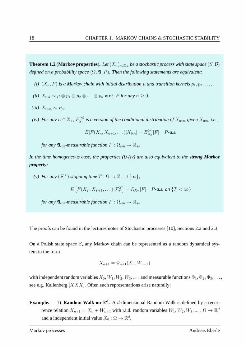
Theorem 1.2(Markov properties ). Let(Xn)n∈Z+ be a stochastic process with state space(S,B)defined on a probability space(Ω,A, P ). Then the following statements are equivalent:
(i) (Xn, P ) is a Markov chain with initial distributionµ and transition kernelsp1, p2, . . . .
(ii) X0:n ∼ µ⊗ p1 ⊗ p2 ⊗ · · · ⊗ pn w.r.t. P for anyn ≥ 0.
(iii) X0:∞ ∼ Pµ.
(iv) For anyn ∈ Z+, P (n)Xn
is a version of the conditional distribution ofXn:∞ givenX0:n, i.e.,
E[F (Xn, Xn+1, . . . )|X0:n] = E(n)Xn
[F ] P -a.s.
for anyAcan-measurable functionF : Ωcan → R+.
In the time homogeneous case, the properties (i)-(iv) are also equivalent to thestrong Markov
property:
(v) For any(FXn ) stopping timeT : Ω → Z+ ∪ ∞,
E[F (XT , XT+1, . . . )|FX
T
]= EXT
[F ] P -a.s. onT <∞
for anyAcan-measurable functionF : Ωcan → R+.
The proofs can be found in the lectures notes of Stochastic processes [10], Sections 2.2 and 2.3.
On a Polish state spaceS, any Markov chain can be represented as a random dynamical sys-
tem in the form
Xn+1 = Φn+1(Xn,Wn+1)
with independent random variablesX0,W1,W2,W3, . . . and measurable functionsΦ1,Φ2,Φ3, . . . ,
see e.g. Kallenberg[XXX]. Often such representations arise naturally:
Example. 1) Random Walk on Rd. A d-dimensional Random Walk is defined by a recur-
rence relationXn+1 = Xn +Wn+1 with i.i.d. random variablesW1,W2,W3, ... : Ω → Rd
and a independent initial valueX0 : Ω → Rd.
Markov processes Andreas Eberle
1.1. TRANSITION PROBABILITIES AND MARKOV CHAINS 19
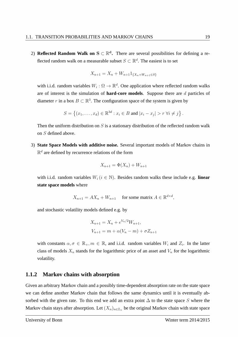
2) Reflected Random Walk onS ⊂ Rd. There are several possibilities for defining a re-
flected random walk on a measurable subsetS ⊂ Rd. The easiest is to set
Xn+1 = Xn +Wn+11Xn+Wn+1∈S
with i.i.d. random variablesWi : Ω → Rd. One application where reflected random walks
are of interest is the simulation ofhard-core models. Suppose there ared particles of
diameterr in a boxB ⊂ R3. The configuration space of the system is given by
S =(x1, . . . , xd) ∈ R3d : xi ∈ B and|xi − xj| > r ∀i 6= j
.
Then the uniform distribution onS is a stationary distribution of the reflected random walk
onS defined above.
3) State Space Models with additive noise.Several important models of Markov chains in
Rd are defined by recurrence relations of the form
Xn+1 = Φ(Xn) +Wn+1
with i.i.d. random variablesWi (i ∈ N). Besides random walks these include e.g.linear
state space modelswhere
Xn+1 = AXn +Wn+1 for some matrixA ∈ Rd×d,
and stochastic volatility models defined e.g. by
Xn+1 = Xn + eVn/2Wn+1,
Vn+1 = m+ α(Vn −m) + σZn+1
with constantsα, σ ∈ R+,m ∈ R, and i.i.d. random variablesWi andZi. In the latter
class of modelsXn stands for the logarithmic price of an asset andVn for the logarithmic
volatility.
1.1.2 Markov chains with absorption
Given an arbitrary Markov chain and a possibly time-dependent absorption rate on the state space
we can define another Markov chain that follows the same dynamics until it is eventually ab-
sorbed with the given rate. To this end we add an extra point∆ to the state spaceS where the
Markov chain stays after absorption. Let(Xn)n∈Z+ be the original Markov chain with state space
University of Bonn Winter term 2014/2015
20 CHAPTER 1. MARKOV CHAINS & STOCHASTIC STABILITY
S and transition probabilitiespn, and suppose that the absorption rates are given by measurable
functionswn : S × S → [0,∞], i.e., the survival (non-absorption) probability ise−wn(x,y) if the
Markov chain is jumping fromx to y in the n-th step. LetEn (n ∈ N) be independent exponential
random variables with parameter1 that are also independent of the Markov chain(Xn). Then we
can define the absorbed chains with state spaceS∪∆ recursively byXw0 = X0,
Xwn+1 =
Xn if Xw
n 6= ∆ and En+1 ≥ wn(Xn, Xn+1),
∆ otherwise.
Example (Absorption at the boundary). If D is a measurable subset ofS and we set
wn(x, y) =
0 for y ∈ D,
∞ for y ∈ S\D,
then the Markov chain is absorbed completely when exiting the domainD for the first time.
Lemma 1.3(Absorbed Markov chain). The process(Xwn ) is a Markov chain onS∆ w.r.t. the
filtration Fn = σ(X0, X1, . . . , Xn, E1, . . . , En). The transition probabilities are given by
Pwn (x, dy) = e−wn(x,y)pn(x, dy) +
(1−ˆ
e−wn(x,z)pn(x, dz)
)δ∆(dy) for x ∈ S.
Pwn (∆, ·) = δ∆
Proof. For any Borel subsetB of S,
P[Xw
n+1 ∈ B|Fn
]= E [P [Xn+1 ∈ B,En+1 ≥ wn(Xn, Xn+1)|σ(X0:∞, E1:n)] |Fn]
= E[1B(Xn+1)e
−wn(Xn,Xn+1)|X0:n
]
=
ˆ
B
e−wn(Xn,y)pn(Xn, dy).
Here we have used the properties of conditional expectations and the Markov property for(Xn).
The assertion follows since theσ-algebra onS ∪ ∆ is generated by the sets inB, andB is
stable under intersections.
1.2 Generators and martingales
Let (Xn, Px) be a time-homogeneous Markov chain with transition probability p and initial dis-
tributionX0 = x Px-almost surely for anyx ∈ S.
Markov processes Andreas Eberle
1.2. GENERATORS AND MARTINGALES 21
1.2.1 Generator
The average change off(Xn) in one transition step of the Markov chain starting atx is given by
(Lf)(x) = Ex[f(X1)− f(X0)] =
ˆ
p(x, dy)(f(y)− f(x)). (1.2.1)
Definition (Generator of a time-homogeneous Markov chain).
The linear operatorL : Fb(S) → Fb(S) defined by(1.2.1)is called thegeneratorof the Markov
chain(Xn, Px).
Examples. 1) Simple random walk onZ. Herep(x, ·) = 12δx+1 +
12δx−1. Hence the gener-
ator is given by
(Lf)(x) = 1
2(f(x+ 1) + f(x− 1))−f(x) = 1
2[(f(x+ 1)− f(x))− (f(x)− f(x− 1))] .
2) Random walk onRd. A random walk onRd with increment distributionµ can be repre-
sented as
Xn = x+n∑
k=1
Wk (n ∈ Z+)
with independent random variablesWk ∼ µ. The generator is given by
(Lf)(x) =ˆ
f(x+ w)µ(dw)− f(x) =
ˆ
(f(x+ w)− f(x))µ(dw).
3) Markov chain with absorption. Suppose thatL is the generator of a time-homogeneous
Markov chain with state spaceS. Then the generator of the corresponding Markov chain
onS∪∆ with absorption ratew(x, y) is given by
(Lwf)(x) = (pwf)(x)− f(x) = p(e−w(x,·)f
)− f(x)
= L(e−w(x,·)f
)(x) +
(e−w(x,x) − 1
)f(x)
for any bounded functionf : S ∪ ∆ → R with f(0) = 0, and for anyx ∈ S.
1.2.2 Martingale problem
The generator can be used to identify martingales associated to a Markov chain. Indeed if(Xn, P )
is an(Fn) Markov chain with transition kernelp then forf ∈ Fb(S),
E [f(Xk+1)− f(Xk)|Fk] = EXk[f(X1)− f(X0)] = (Lf)(Xk) P -a.s.∀k ≥ 0.
University of Bonn Winter term 2014/2015
22 CHAPTER 1. MARKOV CHAINS & STOCHASTIC STABILITY
Hence the processM [f ] defined by
M [f ]n = f(Xn)−
n−1∑
k=0
(Lf)(Xk), n ∈ Z+, (1.2.2)
is an(Fn) martingale. We even have:
Theorem 1.4(Martingale problem characterization of Markov chains). LetXn : Ω → S be
an (Fn) adapted stochastic process defined on a probability space(Ω,A, P ). Then(Xn, P ) is
an (Fn) Markov chain with transition kernelp if and only ifM [f ], defined by(1.2.2)is an (Fn)
martingale for any functionf ∈ Fb(S).
The proof is left as an exercise.
The result in Theorem 1.4 can be extended to the time-inhomogeneous case. Indeed, if(Xn, P )
is an inhomogeneous Markov chain with state spaceS and transition kernelspn, n ∈ N, then
the time-space processXn := (n,Xn) is a time-homogeneous Markov chains with state space
Z+ × S. Let
(Lf)(n, x) =ˆ
pn+1(x, dy)(f(n+ 1, y)− f(n, y))
= Ln+1f(n+ 1, ·)(x) + f(n+ 1, x)− f(n, x)
denote the correspondingtime-space generator.
Corollary 1.5 (Time-dependent martingale problem). LetXn : Ω → S be an(Fn) adapted
stochastic process defined on a probability space(Ω,A, P ). Then(Xn, P ) is an (Fn) Markov
chain with transition kernelsp1, p2, . . . if and only if the processes
M [f ]n := f(n,Xn)−
n−1∑
k=0
(Lf)(k,Xk) (n ∈ Z+)
are (Fn) martingales for all bounded functionsf ∈ Fb(Z+ × S).
Proof. By definition, the process(Xn, P ) is a Markov chain with transition kernelspn if and
only if the time-space process((n,Xn), P ) is a time-homogeneous Markov chain with transition
kernel
p((n, x), ·) = δn+1 ⊗ pn+1(x, ·).
The assertion now follows from Theorem 1.4.
Markov processes Andreas Eberle
1.2. GENERATORS AND MARTINGALES 23
In applications it is often not possible to identify relevant martingales explicitly. Instead one
is frequently using supermartingales (or, equivalently, submartingales) to derive upper or lower
bounds on expectation values one is interested in. It is thenconvenient to drop the integrability
assumption in the martingale definition:
Definition (Non-negative supermartingale). A real-valued stochastic process(Mn, P ) is called
a non-negative supermartingalew.r.t. a filtration(Fn) if and only if for anyn ∈ Z+,
(i) Mn ≥ 0 P -almost surely,
(ii) Mn is Fn-measurable, and
(iii) E[Mn+1|Fn] ≤Mn P -almost surely.
The optional stopping theorem and the supermartingale convergence theorem have versions for
non-negative supermartingales. Indeed by Fatou’s lemma,
E[MT ;T <∞] ≤ lim infn→∞
E[MT∧n] ≤ E[M0]
holds for anarbitrary (Fn) stopping timeT : Ω → Z+ ∪ ∞. Similarly, the limit
M∞ = limn→∞
Mn
exists almost surely in[0,∞).
1.2.3 Potential theory for Markov chains
Let (Xn, Px) be a canonical time-homogeneous Markov chain with state space(S,B) and
generator
(Lf)(x) = (pf)(x)− f(x) = Ex[f(X1)− f(X0)]
By Theorem 1.4,
M [f ]n = f(Xn)−
∑
i<n
(Lf)(Xi)
is a martingale w.r.t.(FXn ) andPx for anyx ∈ S andf ∈ Fb(S). Similarly, one easily verifies
that if the inequalityLf ≤ −c holds for non-negative functionsf, c ∈ F+(S), then the process
M [f,c]n = f(Xn) +
∑
i<n
c(Xi)
is a non-negative supermartingale w.r.t.(FXn ) andPx for any x ∈ S. By applying optional
stopping to these processes, we will derive upper bounds forvarious expectations of the Markov
University of Bonn Winter term 2014/2015

24 CHAPTER 1. MARKOV CHAINS & STOCHASTIC STABILITY
chain.
LetD ∈ B be a measurable subset ofS. We define theexterior boundary ofD w.r.t. the Markov
chain as
∂D =⋃
x∈Dsuppp(x, ·) \D
where the support supp(µ) of a measureµ on (S,B) is defined as the smallest closed set A such
thatµ vanishes onAc. Thus, open sets contained in the complement ofD∪∂D can not be reached
by the Markov chain in a single transition step fromD.
Examples. (1). For the simple random walk onZd, the exterior boundary of a subsetD ⊂ Zd
is given by
∂D = x ∈ Zd \D : |x− y| = 1 for somey ∈ D.
(2). For the ball walk onRd with transition kernel
p(x, ·) = Unif (B(x, r)) ,
the exterior boundary of a Borel setD ∈ B is ther-neighbourhood
∂D = x ∈ Rd \D : dist(x,D) ≤ r.
Let
T = minn ≥ 0 : Xn ∈ Dc
denote the first exit time fromD. Then
XT ∈ ∂D Px-a.s. onT <∞ for anyx ∈ D.
Our aim is to compute or bound expectations of the form
u(x) = Ex
[e−
T−1∑
n=0w(Xn)
f(XT );T <∞]+ Ex
[T−1∑
n=0
e−
n−1∑
i=0w(Xi)
c(Xn)
](1.2.3)
for given non-negative measurable functionsf : ∂D → R+, c, w : D → R+. The general
expression (1.2.3) combines a number of important probabilities and expectations related to the
Markov chain:
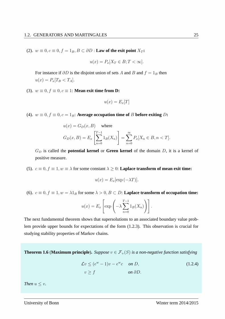
Examples. (1). w ≡ 0, c ≡ 0, f ≡ 1: Exit probability from D:
u(x) = Px[T <∞]
Markov processes Andreas Eberle
1.2. GENERATORS AND MARTINGALES 25
(2). w ≡ 0, c ≡ 0, f = 1B, B ⊂ ∂D : Law of the exit point XT :
u(x) = Px[XT ∈ B;T <∞].
For instance if∂D is the disjoint union of setsA andB andf = 1B then
u(x) = Px[TB < TA].
(3). w ≡ 0, f ≡ 0, c ≡ 1: Mean exit time from D:
u(x) = Ex[T ]
(4). w ≡ 0, f ≡ 0, c = 1B: Average occupation time ofB before exitingD:
u(x) = GD(x,B) where
GD(x,B) = Ex
[T−1∑
n=0
1B(Xn)
]=
∞∑
n=0
Px[Xn ∈ B, n < T ].
GD is called thepotential kernel or Green kernel of the domainD, it is a kernel of
positive measure.
(5). c ≡ 0, f ≡ 1, w ≡ λ for some constantλ ≥ 0: Laplace transform of mean exit time:
u(x) = Ex[exp (−λT )].
(6). c ≡ 0, f ≡ 1, w = λ1B for someλ > 0, B ⊂ D: Laplace transform of occupation time:
u(x) = Ex
[exp
(−λ
T−1∑
n=0
1B(Xn)
)].
The next fundamental theorem shows that supersolutions to an associated boundary value prob-
lem provide upper bounds for expectations of the form (1.2.3). This observation is crucial for
studying stability properties of Markov chains.
Theorem 1.6(Maximum principle ). Supposev ∈ F+(S) is a non-negative function satisfying
Lv ≤ (ew − 1)v − ewc onD, (1.2.4)
v ≥ f on∂D.
Thenu ≤ v.
University of Bonn Winter term 2014/2015
26 CHAPTER 1. MARKOV CHAINS & STOCHASTIC STABILITY
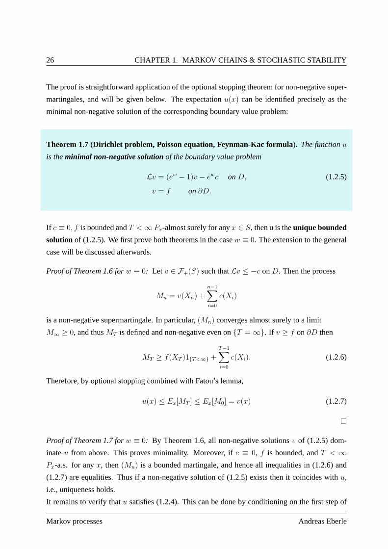
The proof is straightforward application of the optional stopping theorem for non-negative super-
martingales, and will be given below. The expectationu(x) can be identified precisely as the
minimal non-negative solution of the corresponding boundary value problem:
Theorem 1.7(Dirichlet problem, Poisson equation, Feynman-Kac formula). The functionu
is theminimal non-negative solutionof the boundary value problem
Lv = (ew − 1)v − ewc onD, (1.2.5)
v = f on∂D.
If c ≡ 0, f is bounded andT <∞ Px-almost surely for anyx ∈ S, then u is theunique bounded
solution of (1.2.5). We first prove both theorems in the casew ≡ 0. The extension to the general
case will be discussed afterwards.
Proof of Theorem 1.6 forw ≡ 0: Let v ∈ F+(S) such thatLv ≤ −c onD. Then the process
Mn = v(Xn) +n−1∑
i=0
c(Xi)
is a non-negative supermartingale. In particular,(Mn) converges almost surely to a limit
M∞ ≥ 0, and thusMT is defined and non-negative even onT = ∞. If v ≥ f on∂D then
MT ≥ f(XT )1T<∞ +T−1∑
i=0
c(Xi). (1.2.6)
Therefore, by optional stopping combined with Fatou’s lemma,
u(x) ≤ Ex[MT ] ≤ Ex[M0] = v(x) (1.2.7)
Proof of Theorem 1.7 forw ≡ 0: By Theorem 1.6, all non-negative solutionsv of (1.2.5) dom-
inateu from above. This proves minimality. Moreover, ifc ≡ 0, f is bounded, andT < ∞Px-a.s. for anyx, then(Mn) is a bounded martingale, and hence all inequalities in (1.2.6) and
(1.2.7) are equalities. Thus if a non-negative solution of (1.2.5) exists then it coincides withu,
i.e., uniqueness holds.
It remains to verify thatu satisfies (1.2.4). This can be done by conditioning on the first step of
Markov processes Andreas Eberle
1.2. GENERATORS AND MARTINGALES 27
the Markov chain: Forx ∈ D, we haveT ≥ 1 Px-almost surely. In particular, ifT <∞ thenXT
coincides with the exit point of the shifted Markov chain(Xn+1)n≥0, andT − 1 is the exit time
of (Xn+1). Therefore, the Markov property implies that
Ex
[f(XT )1T<∞ +
∑
n<T
c(Xn)|X1
]
= c(x) + Ex
[f(XT )1T<∞ +
∑
n<T−1
c(Xn+1)|X1
]
= c(x) + EX1
[f(XT )1T<∞ +
∑
n<T
c(Xn)
]
= c(x) + u(X1) Px-almost surely,
and hence
u(x) = Ex [c(x) + u(X1)] = c(x) + (pu)(x),
i.e., Lu(x) = −c(x).
Moreover, forx ∈ ∂D, we haveT = 0 Px-almost surely and hence
u(x) = Ex[f(X0)] = f(x).
We now extend the results to the casew 6≡ 0. This can be done by representing the expectation
in (1.2.5) as a corresponding expectation withw ≡ 0 for an absorbed Markov chain:
Reduction of general case tow ≡ 0: We consider the Markov chain(Xwn ) with absorption rate
w defined on the extended state spaceS∪∆ byXw0 = X0,
Xwn+1 =
Xn+1 if Xw
n 6= ∆ andEn+1 ≥ w(Xn),
∆ otherwise,
with independent Exp(1) distributed random variablesEi(i ∈ N) that are independent of(Xn) as
well. Settingf(∆) = c(∆) = 0 one easily verifies that
u(x) = Ex[f(XwT );T <∞] + Ex[
T−1∑
n=0
c(Xwn )].
By applying Theorem 1.6 and 1.7 withw ≡ 0 to the Markov chain(Xwn ), we see thatu is the
minimal non-negative solution of
Lwu = −c onD, u = f on∂D, (1.2.8)
University of Bonn Winter term 2014/2015
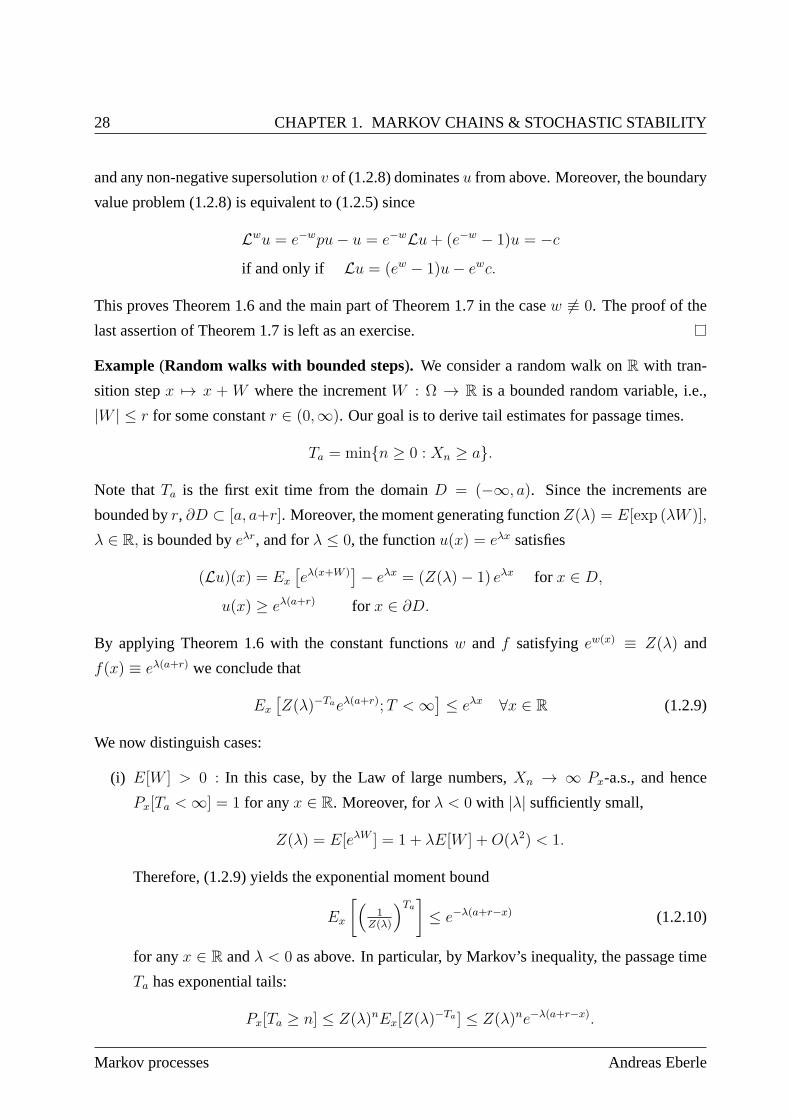
28 CHAPTER 1. MARKOV CHAINS & STOCHASTIC STABILITY
and any non-negative supersolutionv of (1.2.8) dominatesu from above. Moreover, the boundary
value problem (1.2.8) is equivalent to (1.2.5) since
Lwu = e−wpu− u = e−wLu+ (e−w − 1)u = −cif and only if Lu = (ew − 1)u− ewc.
This proves Theorem 1.6 and the main part of Theorem 1.7 in thecasew 6≡ 0. The proof of the
last assertion of Theorem 1.7 is left as an exercise.
Example (Random walks with bounded steps). We consider a random walk onR with tran-
sition stepx 7→ x +W where the incrementW : Ω → R is a bounded random variable, i.e.,
|W | ≤ r for some constantr ∈ (0,∞). Our goal is to derive tail estimates for passage times.
Ta = minn ≥ 0 : Xn ≥ a.
Note thatTa is the first exit time from the domainD = (−∞, a). Since the increments are
bounded byr, ∂D ⊂ [a, a+r]. Moreover, the moment generating functionZ(λ) = E[exp (λW )],
λ ∈ R, is bounded byeλr, and forλ ≤ 0, the functionu(x) = eλx satisfies
(Lu)(x) = Ex
[eλ(x+W )
]− eλx = (Z(λ)− 1) eλx for x ∈ D,
u(x) ≥ eλ(a+r) for x ∈ ∂D.
By applying Theorem 1.6 with the constant functionsw and f satisfyingew(x) ≡ Z(λ) and
f(x) ≡ eλ(a+r) we conclude that
Ex
[Z(λ)−Taeλ(a+r);T <∞
]≤ eλx ∀x ∈ R (1.2.9)
We now distinguish cases:
(i) E[W ] > 0 : In this case, by the Law of large numbers,Xn → ∞ Px-a.s., and hence
Px[Ta <∞] = 1 for anyx ∈ R. Moreover, forλ < 0 with |λ| sufficiently small,
Z(λ) = E[eλW ] = 1 + λE[W ] +O(λ2) < 1.
Therefore, (1.2.9) yields the exponential moment bound
Ex
[(1
Z(λ)
)Ta]≤ e−λ(a+r−x) (1.2.10)
for anyx ∈ R andλ < 0 as above. In particular, by Markov’s inequality, the passage time
Ta has exponential tails:
Px[Ta ≥ n] ≤ Z(λ)nEx[Z(λ)−Ta ] ≤ Z(λ)ne−λ(a+r−x).
Markov processes Andreas Eberle
1.3. LYAPUNOV FUNCTIONS AND RECURRENCE 29
(ii) E[W ] = 0 : In this case, we may haveZ(λ) ≥ 1 for anyλ ∈ R, and thus we can not
apply the argument above. Indeed, it is well known that for instance for the simple random
walk onZ even the first momentEx[Ta] is infinite, cf. [Eberle:Stochastic processes] [10].
However, we may apply a similar approach as above to the exit timeTR\(−a,a) from a finite
interval. We assume thatW has a symmetric distribution, i.e.,W ∼ −W . By choosing
u(x) = cos(λx) for someλ > 0 with λ(a+ r) < π/2, we obtain
(Lu)(x) = E[cos(λx+W )]− cos(λx)
= cos(λx)E[cos(λW )] + sin(λx)E[sin(λW )]− cos(λx)
= (C(λ)− 1) cos(λx)
whereC(λ) := E[cos(λW )], andcos(λx) ≥ cos (λ(a+ r)) > 0 for x ∈ ∂(−a, a). Here
we have used that∂(−a, a) ⊂ [−a − r, a + r] andλ(a + r) < π/2. If W does not vanish
almost surely thenC(λ) < 1 for sufficiently smallλ. Hence we obtain similarly as above
the exponential tail estimate
Px
[T(−a,a)c ≥ n
]≤ C(λ)nE
[C(λ)−T(−a,a)c
]≤ C(λ)n
cos(λx)
cos(λ(a+ r))for |x| < a.
1.3 Lyapunov functions and recurrence
The results in the last section already indicated that superharmonic functions can be used to con-
trol stability properties of Markov chains, i.e., they can serve as stochastic Lyapunov functions.
This idea will be developed systematically in this and the next sections. As before we consider a
time-homogeneous Markov chain(Xn, Px) with generatorL = p − I on a Polish state spaceS
endowed with the Borelσ-algebraB. We start with the following simple observation:
Lemma 1.8. [Locally Superharmonic functions and supermartingales] LetA ∈ B and suppose
thatV ∈ F+(S) is a non-negative function satisfying
LV ≤ −c onS \ A
for some constantc ≥ 0. Then the process
Mn = V (Xn∧TA) + c · (n ∧ TA) (1.3.1)
is a non-negative supermartingale.
The elementary proof is left as an exercise.
University of Bonn Winter term 2014/2015
30 CHAPTER 1. MARKOV CHAINS & STOCHASTIC STABILITY
1.3.1 Recurrence of sets
The first return time to a setA is given by
T+A = infn ≥ 1 : Xn ∈ A.
Notice that
TA = T+A · 1X0 /∈A,
i.e., the first hitting time and the first return time coincideif and only if the chain is not started in
A.
Definition (Harris recurrence and positive recurrence). A setA ∈ B is calledHarris recur-
rent iff
Px[T+A <∞] = 1 for anyx ∈ A.
It is calledpositive recurrentiff
Ex[T+A ] <∞ for anyx ∈ A.
The name “Harris recurrence” is used to be able to differentiate between several possible notions
of recurrence that are all equivalent on a discrete state space but not necessarily on a general state
space, cf. [Meyn and Tweedie: Markov Chains and Stochastic Stability] [23]. Harris recurrence
is the most widely used notion of recurrence on general statespaces. By the strong Markov
property, the following alternative characterisations holds:
Exercise. Prove that a setA ∈ B is Harris recurrent if and only if
Px[Xn ∈ A infinitely often] = 1 for anyx ∈ A
We will now show that the existence of superharmonic functions with certain properties provides
sufficient conditions for non-recurrence, Harris recurrence and positive recurrence respectively.
Below, we will see that for irreducible Markov chains on countable spaces these conditions are
essentially sharp. The conditions are:
(LT) There exists a functionV ∈ F+(S) andy ∈ S such that
LV ≤ 0 onAc andV (y) < infAV.
(LR) There exists a functionV ∈ F+(S) such that
LV ≤ 0 onAc andTV >c <∞ Px-a.s. for anyx ∈ S andc ≥ 0.
Markov processes Andreas Eberle
1.3. LYAPUNOV FUNCTIONS AND RECURRENCE 31
(LP) There exists a functionV ∈ F+(S) such that
LV ≤ −1 onAc andpV <∞ onA.
Theorem 1.9. (Foster-Lyapunov conditions for non-recurrence, Harris recurrence and
positive recurrence)
(1). If (LT ) holds then
Py[TA <∞] ≤ V (y)/ infAV < 1.
(2). If (LR) holds then
Px[TA <∞] = 1 for anyx ∈ S.
In particular, the setA is Harris recurrent.
(3). If (LP ) holds then
Ex[TA] ≤ V (x) <∞ for anyx ∈ Ac, and
Ex[T+A ] ≤ (pV )(x) <∞ for anyx ∈ A.
In particular, the setA is positive recurrent.
Proof: (1). If LV ≤ 0 onAc then by Lemma 1.8 the processMn = V (Xn∧TA) is a non-negative
supermartingale w.r.t.Px for any x. Hence by optional stopping and Fatou’s lemma,
V (y) = Ey[M0] ≥ Ey[MTA;TA <∞] ≥ Py[TA <∞] · inf
AV.
Assuming(LT ), we obtainPy[TA <∞] < 1.
(2). Now assume that(LR) holds. Then by applying optional stopping to(Mn), we obtain
V (x) = Ex[M0] ≥ Ex[MTV >c] = Ex[V (XTA∧TV >c
)] ≥ cPx[TA = ∞]
for any c > 0 andx ∈ S. Here we have used thatTV >c < ∞ Px-almost surely and
henceV (XTA∧TV >c) ≥ c Px-almost surely onTA = ∞. By letting c tend to infinity,
we conclude thatPx[TA = ∞] = 0 for anyx.
(3). Finally, suppose thatLV ≤ −1 onAc. Then by Lemma 1.8,
Mn = V (Xn∧TA) + n ∧ TA
University of Bonn Winter term 2014/2015

32 CHAPTER 1. MARKOV CHAINS & STOCHASTIC STABILITY
is a non-negative supermartingale w.r.t.Px for anyx. In particular,(Mn) convergesPx-
almost surely to a finite limit, and hencePx[TA < ∞] = 1. Thus by optional stopping and
sinceV ≥ 0,
Ex[TA] ≤ Ex[MTA] ≤ Ex[M0] = V (x) for anyx ∈ S. (1.3.2)
Moreover, we can also estimate the first return time by conditioning on the first step. In-
deed, forx ∈ A we obtain by (1.3.2):
Ex[T+A ] = Ex
[Ex[T
+A |X1]
]= Ex [EX1 [TA]] ≤ Ex[V (X1)] = (pV )(x)
ThusA is positive recurrent if(LP ) holds.
Example (State space model onRd). We consider a simple state space model with one-step
transition
x 7→ x+ b(x) +W
whereb : Rd → Rd is a measurable vector field andW : Ω → Rd is a square-integrable random
vector withE[W ] = 0 andCov(W i,W j) = δij. As a Lyapunov function we try
V (x) = |x|/ε for some constantε > 0.
A simple calculation shows that
ε(LV )(x) = E[|x+ b(x) +W |2
]− |x|2
= |x+ b(x)|2 + E[|W |2]− |x|2 = 2x · b(x) + |b(x)|2 + d.
Therefore, the conditionLV (x) ≤ −1 is satisfied if and only if
2x · b(x) + |b(x)|2 + d ≤ −ε.
By choosingε small enough we see that positive recurrence holds for ballB(0, r) with r suffi-
ciently large provided
lim sup|x|→∞
(2x · b(x) + |b(x)|2
)< −d. (1.3.3)
This condition is satisfied in particular if outside of a ball, the radial componentbr(x) = x|x| · b(x)
of the drift satisfies(1− δ)br(x) ≤ − d2|x| for someδ > 0, and|b(x)|2/r ≤ −δ · br(x).
Markov processes Andreas Eberle
1.3. LYAPUNOV FUNCTIONS AND RECURRENCE 33
Exercise. Derive a sufficient condition similar to (1.3.3) for positive recurrence of state space
models with transition step
x 7→ x+ b(x) + σ(x)W
whereb andW are chosen as in the example above andσ is a measurable function fromRd to
Rd×d.
Example(Recurrence and transience for the simple random walk onZd). The simple random
walk is the Markov chain onZd with transition probabilitiesp(x, y) = 12d
if |x − y| = 1 and
p(x, y) = 0 otherwise. The generator is given by
(Lf)(x) = 1
2d(∆Zdf)(x) =
1
2d
d∑
i=1
[(f(x+ ei)− f(x))− (f(x)− f(x− ei))] .
In order to find suitable Lyapunov functions, we approximatethe discrete Laplacian onZd by the
Laplacian onRd. By Taylor’s theorem, forf ∈ C4(Rd),
f(x+ ei)− f(x) = ∂if(x) +1
2∂2iif(x) +
1
6∂3iiif(x) +
1
24∂4iiiif(ξ),
f(x− ei)− f(x) = −∂if(x) +1
2∂2iif(x)−
1
6∂3iiif(x) +
1
24∂4iiiif(η),
whereξ andη are intermediate points on the line segments betweenx andx + ei, x andx − ei
respectively. Adding these2d equations, we see that
∆Zdf(x) = ∆f(x) +R(x), where (1.3.4)
|R(x)| ≤ d
12supB(x,1)
‖∂4f‖. (1.3.5)
This suggests to choose Lyapunov functions that are close toharmonic functions onRd outside a
ball. However, since there is a perturbation involved, we will not be able to use exactly harmonic
functions, but we will have to choose functions that are strictly superharmonic instead. We try
V (x) = |x|p for somep ∈ R.
By the expression for the Laplacian in polar coordinates,
∆V (x) =
(d2
dr2+d− 1
r
d
dr
)rp
= p · (p− 1 + d− 1) rp−2
University of Bonn Winter term 2014/2015
34 CHAPTER 1. MARKOV CHAINS & STOCHASTIC STABILITY
wherer = |x|. In particular,V is superharmonic onRd if and only ifp ∈ [0, 2−d] or p ∈ [2−d, 0]respectively. The perturbation term can be controlled by noting that there exists a finite constant
C such that
‖∂4V (x)‖ ≤ C · |x|p−4 (Exercise).
This bound shows that the approximation of the discrete Laplacian by the Laplacian onRd im-
proves if|x| is large. Indeed by (1.3.4) and (1.3.5) we obtain
LV (x) =1
2d∆ZdV (x)
≤ p
2d(p+ d− 2)rp−2 +
C
2drp−4.
ThusV is superharmonic forL outside a ball providedp ∈ (0, 2−d) orp ∈ (2−d, 0) respectively.
We now distinguish cases:
d > 2 : In this case we can choosep < 0 such thatLV ≤ 0 outside some ballB(0, r0). Sincerp
is decreasing, we have
V (x) < infB(0,r0)
V for anyx with |x| > r0,
and hence by Theorem 1.9,
Px[TB(0,r0) <∞] < 1 whenever|x| > r0.
Theorem 1.10 below shows that this implies that any finite setis transient, i.e., it is almost
surely visited only finitely many times by the random walk with an arbitrary starting point.
d < 2 : In this case we can choosep ∈ (0, 2 − d) to obtainLV ≤ 0 outside some ballB(0, r0).
Now V (x) → ∞ as|x| → ∞. Sincelim sup |Xn| = ∞ almost surely, we see that
TV >c <∞ Px-almost surely for anyx ∈ Zd andc ∈ R+.
Therefore, by Theorem 1.9, the ballB(0, r0) is (Harris)recurrent . By irreducibility this
implies that any statex ∈ Zd is recurrent, cf. Theorem 1.10 below.
d = 2 : This is the critical case and therefore more delicate. The Lyapunov functions considered
above can not be used. Since a rotationally symmetric harmonic function for the Laplacian
onR2 is log |x|, it is natural to try choosingV (x) = (log |x|)α for someα ∈ R+. Indeed,
one can show by choosing appropriately that the Lyapunov condition for recurrence is
satisfied in this case as well:
Markov processes Andreas Eberle
1.3. LYAPUNOV FUNCTIONS AND RECURRENCE 35
Exercise (Recurrence of the two-dimensional simple random walk). Show by choosing an
appropriate Lyapunov function that the simple random walk onZ2 is recurrent.
Exercise(Recurrence and transience of Brownian motion). A continuous-time stochastic pro-
cess((Bt)t∈[0,∞), Px
)taking values inRd is called aBrownian motion starting at xif the sample
pathst 7→ Bt(ω) are continuous,B0 = x Px-a.s., and for everyf ∈ C2b (R
d), the process
M[f ]t = f(Bt)−
1
2
ˆ t
0
∆f(Bs)ds
is a martingale w.r.t. the filtrationFBt = σ(Bs : s ∈ [0, t]). LetTa = inft ≥ 0 : |Bt| = a.
a) ComputePx[Ta < Tb] for a < |x| < b.
b) Show that ford ≤ 2, a Brownian motion is recurrent in the sense thatPx[Ta <∞] = 1 for
anya < |x|.
c) Show that ford ≥ 3, a Brownian motion is transient in the sense thatPx[Ta < ∞] → 0 as
|x| → ∞.
You may assume the optional stopping theorem and the martingale convergence theorem in con-
tinuous time without proof. You may also assume that the Laplacian applied to a rotationally
symmetric functiong(x) = γ(|x|) is given by
∆g(x) = r1−d d
dr
(rd−1 d
drγ
)(r) =
d2
dr2γ(r) +
d− 1
r
d
drγ(r) wherer = |x|.
(How can you derive this expression rapidly if you do not remember it?)
1.3.2 Global recurrence
For irreducible Markov chains on countable state spaces, recurrence respectively transience of an
arbitrary finite set already implies that recurrence resp. transience holds for any finite set. This
allows to show that the Lyapunov conditions for recurrence and transience are both necessary
and sufficient. On general state spaces this is not necessarily true, and proving corresponding
statements under appropriate conditions is much more delicate. We recall the results on countable
state spaces, and we state a result on general state spaces without proof. For a thorough treatment
of recurrence properties for Markov chains on general statespaces we refer to the monograph
“Markov chains and stochastic stability” by Meyn and Tweedie, [23].
University of Bonn Winter term 2014/2015
36 CHAPTER 1. MARKOV CHAINS & STOCHASTIC STABILITY
a) Countable state space
Suppose thatp(x, y) = p(x, y) are the transition probabilities of a homogeneous Markov chain
(Xn, Px) taking values in a countable setS, and letTy andT+y denote the first hitting resp. return
time to a sety consisting of a single statey ∈ S.
Definition (Irreducibility on countable state spaces). The transition matrixp and the Markov
chain(Xn, Px) are calledirreducible if and only if
(1). ∀x, y ∈ S : ∃n ∈ Z+ : pn(x, y) > 0, or equivalently, if and only if
(2). ∀x, y ∈ S : Px[Ty <∞] > 0.
If the transition matrix is irreducible then recurrence andpositive recurrence of different states
are equivalent to each other, since between two visits to a recurrent state the Markov chain will
visit any other state with positive probability:
Theorem 1.10(Recurrence and positive recurrence of irreducible Markov chains). Suppose
thatS is countable and the transition matrixp is irreducible.
(1). The following statements are all equivalent:
(i) There exists a finite recurrent setA ⊂ S.
(ii) For any x ∈ S, the setx is recurrent.
(iii) For any x, y ∈ S,
Px[Xn = y infinitely often] = 1.
(2). The following statements are all equivalent:
(i) There exists a finite positive recurrent setA ⊂ S.
(ii) For any x ∈ S, the setx is positive recurrent.
(iii) For any x, y ∈ S,
Ex[Ty] <∞.
The proof is left as an exercise, see also the lecture notes on“Stochastic Processes”, [10]. The
Markov chain is called(globally) recurrent iff the equivalent conditions in (1) hold, and tran-
sient iff these conditions do not hold. Similarly, it is called (globally) positive recurrent iff the
Markov processes Andreas Eberle

1.3. LYAPUNOV FUNCTIONS AND RECURRENCE 37
conditions in (2) are satisfied. By the example above, ford ≤ 2 the simple random walk onZd is
globally recurrent but not positive recurrent. Ford ≥ 3 it is transient.
As a consequence of Theorem 1.10, we obtain Lyapunov conditions for transience, recurrence
and positive recurrence on a countable state space that are both necessary and sufficient:
Corollary 1.11 (Foster-Lyapunov conditions for recurrence on a countable state space).
Suppose thatS is countable and the transition matrixp is irreducible. Then:
1) The Markov chain is transient if and only if there exists a finite setA ⊂ S and a function
V ∈ F+(S) such that(LT ) holds.
2) The Markov chain is recurrent if and only if there exists a finite setA ⊂ S and a function
V ∈ F+(S) such that
(LR′) LV ≤ 0 onAc, andV ≤ c is finite for anyc ∈ R+.
3) The Markov chain is positive recurrent if and only if thereexists a finite setA ⊂ S and a
functionV ∈ F+(S) such that(LP ) holds.
Proof: Sufficiency of the Lyapunov conditions follows directly by Theorems 1.9 and 1.10: If
(LT ) holds then by 1.9 there existsy ∈ S such thatPy[TA <∞], and hence the Markov chain is
transient by 1.10. Similarly, if(LP ) holds thenA is positive recurrent by 1.9, and hence global
positive recurrence holds by 1.10. Finally, if(LR′) holds and the state space is not finite, then
for anyc ∈ R+, the setV ≤ c is not empty. Therefore,(LR) holds by irreducibility, and the
recurrence follows again from 1.9 and 1.10. IfS is finite then any irreducible chain is globally
recurrent.
We now prove that the Lyapunov conditions are alsonecessary:
1) If the Markov chain is transient then we can find a statex ∈ S and a finite setA ⊂ S such
that the functionV (x) = Px[TA <∞] satisfies
V (x) < 1 = infAV.
By Theorem 1.7,V is harmonic onAc and thus(LT ) is satisfied.
2) Now suppose that the Markov chain is recurrent. IfS is finite then(LR′) holds withA = S
for an arbitrary functionV ∈ F+(S). If S is not finite then we choose a finite setA ⊂ S
and an arbitrary decreasing sequence of setsDn ⊂ S such thatA ⊂ Dc1, D
cn is finite for
anyn, and⋂Dn = ∅, and we set
Vn(x) = Px[TDn < TA].
University of Bonn Winter term 2014/2015
38 CHAPTER 1. MARKOV CHAINS & STOCHASTIC STABILITY
ThenVn ≡ 1 onDn and asn→ ∞,
Vn(x) ց Px[TA = ∞] = 0 for anyx ∈ S.
SinceS is countable, we can apply a diagonal argument to extract a subsequence such that
V (x) :=∞∑
n=0
Vnk(x) <∞ for anyx ∈ S.
By Theorem 1.7, the functionsVn andV are harmonic onS \A. Moreover,V ≥ k onDnk.
Thus the sub-level sets ofV are finite, and(LR′) is satisfied.
3) Finally if the chain is positive recurrent then for an arbitrary finite setA ⊂ S, the function
V (x) = Ex[TA] is finite and satisfiesLV = −1 onAc. Since
(pV )(x) = Ex [EX1 [TA]] = Ex
[Ex[T
+A |X1]
]= Ex[T
+A ] <∞
for anyx, condition(LP ) is satisfied.
b) Extension to locally compact state spaces
Extensions of Corollary 1.11 to general state spaces are not trivial. Suppose for example thatS
is locally compact, i.e., there exists a sequence of compact setsKn ⊂ S such thatS =⋃n∈N
Kn.
Let p be a transition kernel on(S,B), and letλ be a positive measure on(S,B) with full support,
i.e., λ(B) > 0 for any non-empty open setB ⊂ S. For instance,S = Rd andλ the Lebesgue
measure.
Definition (λ-irreducibility and Feller property ).
1) The transition kernelp is calledλ-irreducible if and only if for anyx ∈ S and for any
Borel setA ∈ B with λ(A) > 0, there existsn ∈ Z+ such thatpn(x,A) > 0.
2) p is calledFeller iff
(F) pf ∈ Cb(S) for anyf ∈ Cb(S)
One of the difficulties on general state spaces is that there are different concepts of irreducibility.
In general,λ-irreducibility is a strictly stronger condition thantopological irreducibility which
Markov processes Andreas Eberle
1.3. LYAPUNOV FUNCTIONS AND RECURRENCE 39
means that every non-empty open setB ⊂ S is accessible from any statex ∈ S.
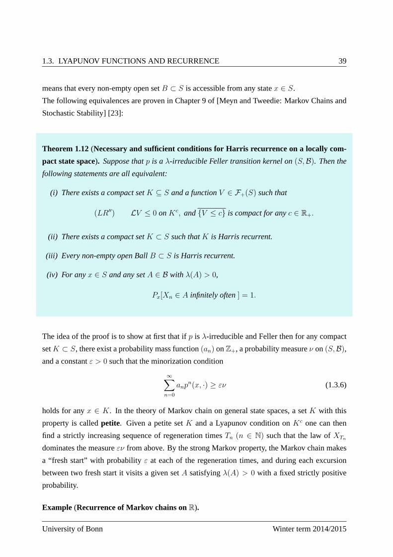
The following equivalences are proven in Chapter 9 of [Meyn and Tweedie: Markov Chains and
Stochastic Stability] [23]:
Theorem 1.12(Necessary and sufficient conditions for Harris recurrence on a locally com-
pact state space). Suppose thatp is aλ-irreducible Feller transition kernel on(S,B). Then the
following statements are all equivalent:
(i) There exists a compact setK ⊆ S and a functionV ∈ F+(S) such that
(LR′′) LV ≤ 0 onKc, andV ≤ c is compact for anyc ∈ R+.
(ii) There exists a compact setK ⊂ S such thatK is Harris recurrent.
(iii) Every non-empty open BallB ⊂ S is Harris recurrent.
(iv) For anyx ∈ S and any setA ∈ B with λ(A) > 0,
Px[Xn ∈ A infinitely often] = 1.
The idea of the proof is to show at first that ifp is λ-irreducible and Feller then for any compact
setK ⊂ S, there exist a probability mass function(an) onZ+, a probability measureν on(S,B),and a constantε > 0 such that the minorization condition
∞∑
n=0
anpn(x, ·) ≥ εν (1.3.6)
holds for anyx ∈ K. In the theory of Markov chain on general state spaces, a setK with this
property is calledpetite. Given a petite setK and a Lyapunov condition onKc one can then
find a strictly increasing sequence of regeneration timesTn (n ∈ N) such that the law ofXTn
dominates the measureεν from above. By the strong Markov property, the Markov chain makes
a “fresh start” with probabilityε at each of the regeneration times, and during each excursion
between two fresh start it visits a given setA satisfyingλ(A) > 0 with a fixed strictly positive
probability.
Example (Recurrence of Markov chains onR).
University of Bonn Winter term 2014/2015
40 CHAPTER 1. MARKOV CHAINS & STOCHASTIC STABILITY
1.4 The space of probability measures
Our next goal is to study convergence of Markov chains to stationary distributions. To this end
we consider different topologies and metrics on the spaceP(S) of probability measures on a
Polish spaceS endowed with its Borelσ-algebraB. We study and apply weak convergence of
probability measures in this section, and we consider Wasserstein and total variation metrics in
the next two sections. A useful additional reference for this section is [Billingsley:Convergence
of probability measures] [2]. Recall thatP(S) is a convex subset of the vector space
M(S) = αµ+ − βµ− : µ+, µ− ∈ P(S), α, β ≥ 0
consisting of all finite signed measures on(S,B). By M+(S) we denote the set of all (not
necessarily finite) non-negative measures on(S,B). For a measureµ and a measurable function
f we set
µ(f) =
ˆ
fdµ whenever the integral exists.
Definition (Invariant measures, stationary distribution). A measureµ ∈ M+(S) is called
invariant w.r.t. a transition kernelp on (S,B) iff µp = µ, i.e., iffˆ
µ(dx)p(x,B) = µ(B) for anyB ∈ B.
An invariant probability measure is also called astationary (initial) distribution or an equilib-
rium of p.
Exercise. Show that the set of invariant probability measures for a given transition kernelp is a
convex subset ofP(S).
1.4.1 Weak topology
Recall that a sequence(µk)k∈N of probability measures on(S,B) is said toconverge weaklyto
a measureµ ∈ P(S) if and only if
(i) µk(f) → µ(f) for anyf ∈ Cb(S).
ThePortemanteau Theoremstates that weak convergence is equivalent to each of the following
properties:
(ii) µk(f) → µ(f) for any uniformly continuousf ∈ C(S).
(iii) lim supµk(A) ≤ µ(A) for any closed setA ⊂ S.
Markov processes Andreas Eberle
1.4. THE SPACE OF PROBABILITY MEASURES 41
(iv) lim inf µk(O) ≥ µ(O) for any open setO ⊂ S.
(v) lim supµk(f) ≤ µ(f) for any upper semicontinuous functionf : S → R that is bounded
from above.
(vi) lim inf µk(f) ≥ µ(f) for any lower semicontinuous functionf : S → R that is bounded
from below.
(vii) µk(f) → µ(f) for any functionf ∈ Fb(S) that is continuous atµ-almost everyx ∈ S.
For the proof see e.g. [Stroock:Probability Theory: An Analytic View] [34], Theorem 3.1.5, or
[Billingsley:Convergence of probability measures] [2]. Thefollowing observation is crucial for
studying weak convergence on polish spaces:
Remark (Polish spaces as measurable subset of[0, 1]N). Suppose that(S, ) is a separable
metric space, andxn : n ∈ N is a countable dense subset. Then the map
h :S → [0, 1]N
x →(
(x,xn)1+(x,xn)
)n∈N
(1.4.1)
is a homeomorphism fromS to h(S) provided[0, 1]N is endowed with the product topology (i.e.,
the topology corresponding to pointwise convergence). In general,h(S) is a measurable subset
of the compact space[0, 1]N (endowed with the productσ-algebra that is generated by the product
topology). IfS is compact thenh(S) is compact as well. In general,
S ∼= h(S) ⊂ S ⊂ [0, 1]N
whereS := h(S) is compact since it is a closed subset of the compact space[0, 1]N. ThusS can
be viewed as a compactification ofS.
On compact spaces, any sequence of probability measures hasa weakly convergent subsequence.
Theorem 1.13.If S is compact thenP(S) is compact w.r.t. weak convergence.
Proof: Suppose thatS is compact. Then it can be shown based on the remark above thatC(S)
is separable w.r.t. uniform convergence. Thus there existsa sequencegn ∈ C(S) (n ∈ N) such
that‖gn‖sup ≤ 1 for anyn, and the linear span of the functionsgn is dense inC(S).
Now consider an arbitrary sequence(µk)k∈N in P(S). We will show that(µk) has a convergent
University of Bonn Winter term 2014/2015
42 CHAPTER 1. MARKOV CHAINS & STOCHASTIC STABILITY
subsequence. Note first that(µk(gn))k∈N is a bounded sequence of real numbers for anyn. By a
diagonal argument, we can extract a subsequence(µkl)l∈N of (µk)k∈N such thatµkl(gn) converges
asl → ∞ for everyn ∈ N. Since the span of the functionsgn is dense inC(S), this implies that
Λ(f) := liml→∞
µkl(f) (1.4.2)
exists for anyf ∈ C(S). It is easy to verify thatΛ is apositive (i.e.,Λ(f) ≥ 0 wheneverf ≥ 0)
linear functional onC(S) with Λ(1) = 1. Moreover, if(fn)n∈N is a decreasing sequence inC(S)
such thatfn ց 0 pointwise, thenfn → 0 uniformly by compactness ofS, and henceΛ(fn) → 0.
Therefore, there exists a probability measureµ onS such that
Λ(f) = µ(f) for anyf ∈ C(S).
By (1.4.2), the sequence(µkl) converges weakly toµ.
Remark (A metric for weak convergence). Choosing the functiongn as in the proof above, we
see that a sequence(µk)k∈N of probability measures inP(S) converges weakly toµ if and only
if µk(gn) → µ(gn) for anyn ∈ N. Thus weak convergence inP(S) is equivalent to convergence
w.r.t. the metric
d(µ, ν) =∞∑
n=1
2−n|µ(gn)− ν(gn)|.
1.4.2 Prokhorov’s theorem
We now consider the case whereS is a non-compact polish space. By identifyingS with the
imageh(S) under the maph defined by (1.4.1), we can still viewS as a measurable subset of the
compact spaceS:
S ⊂ S ⊂ [0, 1]N.
HenceP(S) can be viewed as a subset of the compact spaceP(S):
P(S) = µ ∈ P(S) : µ(S \ S) = 0 ⊂ P(S).
If µk (k ∈ N) andµ are probability measures onS (that trivially extend toS) then:
µk → µ weakly inP(S) (1.4.3)
⇔ µk(f) → µ(f) for any uniformly continuousf ∈ Cb(S)
⇔ µk(f) → µ(f) for anyf ∈ C(S)
⇔ µk → µ weakly inP(S).
Markov processes Andreas Eberle
1.4. THE SPACE OF PROBABILITY MEASURES 43
ThusP(S) inherits the weak topology fromP(S). The problem is, however, that sinceS is
not necessarily a closed subset ofS, it can happen that a sequence(µk) in P(S) converges to a
probability measureµ on S s.t. µ(S) < 1. To exclude this possibility, the following tightness
condition is required:
Definition (Tightness of collections of probability measures). LetR ⊂ P(S) be a set consist-
ing of probability measures onS. ThenR is calledtight iff for any ε > 0 there exists a compact
setK ⊂ S such that
supµ∈R
µ(S \K) < ε.
Thus tightness means that the measures in the setR are concentrated uniformly on a compact set
up to an arbitrary small positive amount of mass. A setR ⊂ P(S) is calledrelatively compact
iff every sequence inR has a subsequence that converges weakly inP(S).
Theorem 1.14(Prokhorov). Suppose thatS is polish, and letR ⊂ P(S). Then
R is relatively compact⇔ R is tight .
In particular, every tight sequence inP(S) has a weakly convergent subsequence.
We only prove the implication “⇐” that will be the more important one for our purposes. This
implication holds in arbitrary separable metric spaces. For the proof of the converse implication
cf. e.g. [Billingsley:Convergence of probability measures][2].
Proof of “⇐”: Let (µk)k∈N be a sequence inR. We have to show that(µk) has a weakly con-
vergent subsequence inP(S). SinceP(S) is compact by Theorem 1.13, there is a subsequence
(µkl) that converges weakly inP(S) to a probability measureµ on S. We claim that by tightness,
µ(S) = 1 andµkl → µ weakly inP(S). Let ε > 0 be given. Then there exists a compact subset
K of S such thatµkl(K) ≥ 1− ε for anyl. SinceK is compact, it is also a compact and (hence)
closed subset ofS. Therefore, by the Portmanteau Theorem,
µ(K) ≥ lim supl→∞
µkl(K) ≥ 1− ε,
and thus
µ(S \ S) ≤ µ(S \K) ≤ ε.
Letting ε tend to0, we see thatµ(S \ S) = 0. Henceµ ∈ P(S) andµkl → µ weakly inP(S) by
(1.4.3).
University of Bonn Winter term 2014/2015
44 CHAPTER 1. MARKOV CHAINS & STOCHASTIC STABILITY
1.4.3 Existence of invariant probability measures
We now apply Prokhorov’s Theorem to derive sufficient conditions for the existence of an invari-
ant probability measure for a given transition kernelp(x, dy) on (S,B).
Definition (Feller property ). The stochastic kernelp is called(weakly) Felleriff pf is continu-
ous for anyf ∈ Cb(S).
A kernelp is Feller if and only ifx 7→ p(x, ·) is a continuous map fromS toP(S) w.r.t. the weak
topology onP(S). Indeed, by definition,p is Feller if and only if
xn → x⇒ (pf)(xn) → (pf)(x) ∀f ∈ Cb(S).
A topological space is said to beσ-compactiff it is the union of countably many compact subsets.
For example,Rd is σ-compact whereas an infinite dimensional Hilbert space is not σ-compact.
Theorem 1.15(Foguel, Krylov-Bogolionbov). Suppose thatp is a Feller transition kernel on
the Polish spaceS, and letpn := 1n
n−1∑i=0
pi. Then there exists an invariant probability measureµ
of p if one of the following conditions is satisfied for somex ∈ S:
(i) The sequencepn(x, ·) : n ∈ N is tight, or
(ii) S is σ-compact, and there exists a compact setK ⊂ S such that
lim infn→∞
pn(x,K) > 0.
Remark. If (Xn, Px) is a canonical Markov chain with transition kernelp then
pn(x,K) = Ex
[1
n
n−1∑
i=0
1K(Xi)
]
is the average proportion of time spent by the chain in the setK during the firstn steps. Condi-
tions(i) and(ii) say that
(i) ∀ε > 0 ∃K ⊂ S compact:pn(x,K) ≥ 1− ε for all n ∈ N,
(ii) ∃ε > 0, K ⊂ S compact,nk ր ∞: pnk(x,K) ≥ ε for all k ∈ N.
Clearly, the second condition is weaker than the first one in several respects.
Markov processes Andreas Eberle

1.4. THE SPACE OF PROBABILITY MEASURES 45
Proof of Theorem 1.15: (i) Suppose that the sequenceνn := pn(x, ·) is tight for somex ∈ S.
Then by Prokhorov’s Theorem, there exists a subsequenceνnkand a probability measure
µ onS such thatνnk→ µ weakly. We claim thatµp = µ. Indeed for,f ∈ Cb(S) we have
pf ∈ Cb(S) by the Feller property. Therefore,
(µp)(f) = µ(pf) = limk→∞
νnk(pf) = lim
k→∞(νnk
p)(f)
= limk→∞
νnk(f) = µ(f) for anyf ∈ Cb(S),
where the second last equality holds since
νnkp =
1
nk
nk−1∑
i=0
pi+1(x, ·) = νnk− 1
nk
δx +1
nk
pnk(x, ·).
(ii) Now suppose that Condition(ii) holds. We may also assume thatS is a Borel subset of a
compact spaceS. SinceP(S) is compact and(ii) holds, there existsε > 0, a compact set
K ⊂ S, a subsequence(νnk) of (νn), and a probability measureµ on S such that
νnk(K) ≥ ε for anyk ∈ N, and νnk
→ µ weakly inS.
Note that weak convergence inS does not imply weak convergence inS. However
νnk(f) → µ(f) for any compactly supported functionf ∈ C(S), and
µ(S) ≥ µ(K) ≥ lim sup νnk(K) ≥ ε.
Therefore, it can be verified similarly as above that the conditioned measure
µ(B) =µ(B ∩ S)µ(S)
= µ(B|S), B ∈ B(S),
is an invariant probability measure forp.
In practice, the assumptions in Theorem 1.15 can be verified via appropriate Lyapunov functions:
Corollary 1.16 (Lyapunov condition for the existence of an invariant probability measure).
Suppose thatp is a Feller transition kernel andS is σ-compact. Then an invariant probability
measure forp exists if the following Lyapunov condition is satisfied:
(LI) There exists a functionV ∈ F+(S), a compact setK ⊂ S, and constantsc, ε ∈ (0,∞)
such that
LV ≤ c1K − ε.
University of Bonn Winter term 2014/2015
46 CHAPTER 1. MARKOV CHAINS & STOCHASTIC STABILITY
Proof: By (LI),
c1K ≥ ε+ LV = ε+ pV − V.
By integrating the inequality w.r.t. the probability measurepn(x, ·), we obtain
cpn(·, K) = cpn1K ≥ ε+1
n
n−1∑
i=0
(pi+1V − piV )
= ε+1
npnV − 1
nV ≥ ε− 1
nV
for anyn ∈ N. Therefore,
lim infn→∞
pn(x,K) ≥ ε for anyx ∈ S.
The assertion now follows by Theorem 1.15.
Example. 1) Countable state space:If S is countable andp is irreducible then an invariant
probability measure exists if and only if the Markov chain ispositive recurrent. On the other
hand, by Corollary 1.11, positive recurrence is equivalent to (LI). Hence for irreducible
Markov chains on countable state spaces, Condition(LI) is both necessary and sufficient
for the existence of a stationary distribution.
2) S = Rd: OnRd, Condition(LI) is satisfied in particular ifLV is continuous and
lim sup|x|→∞
LV (x) < 0.
1.5 Couplings and transportation metrics
Additional reference: [Villani:Optional transport-old and new] [37].
Let S be a Polish space endowed with its Borelσ-algebraB. An invariant probability measure
is a fixed point of the mapµ 7→ µp acting on an appropriate subspace ofP(S). Therefore, one
approach for studying convergence to equilibrium of Markovchains is to apply the Banach fixed
point theorem and variants thereof. To obtain useful results in this way we need adequate metrics
on probability measures.
1.5.1 Wasserstein distances
We fix a metricd : S × S → [0,∞) on the state spaceS. For p ∈ [1,∞), the space of all
probability measures onS with finite p-th moment is defined by
Pp(S) =
µ ∈ P(S) :
ˆ
d(x0, y)pµ(dy) <∞
,
Markov processes Andreas Eberle
1.5. COUPLINGS AND TRANSPORTATION METRICS 47
wherex0 is an arbitrary given point inS. Note that by the triangle inequality, the definition is
indeed independent ofx0. A natural distance onPp(S) can be defined via couplings:
Definition (Coupling of probability measures). A coupling of measuresµ, ν ∈ Pp(S) is a
probability measureγ ∈ P(S × S) with marginalsµ and ν. The couplingγ is realizedby
random variablesX, Y : Ω → S defined on a common probability space(Ω,A, P ) such that
(X, Y ) ∼ γ.
We denote the set of all couplings of given probability measuresµ andν byΠ(µ, ν).
Definition (Wasserstein distance, Kantorovich distance). For p ∈ [1,∞), theLp Wasserstein
distanceof probability measuresµ, ν ∈ P(S) is defined by
Wp(µ, ν) = infγ∈Π(µ,ν)
(ˆ
d(x, y)pγ(dxdy)
) 1p
= infX∼µ
Y∼ν
E [d(X, Y )p]1p , (1.5.1)
where the second infimum is over all random variablesX, Y defined on a common probability
space with lawsµ andν. TheKantorovich distanceof µ andν is theL1 Wasserstein distance
W1(µ, ν).
Remark (Optimal transport ). The Minimization in (1.5.1) is a particular case of an optimal
transport problem. Given a cost functionc : S × S → [0,∞], one is either looking for a map
T : S → S minimizing the average costˆ
c(x, T (x))µ(dx)
under the constraintν = µ T−1 (Monge problem, 8th century), or, less restrictively, for a
couplingγ ∈ Π(µ, ν) minimizingˆ
c(x, y)γ(dxdy)
(Kantorovich problem , around 1940).
Note that the definition of theWp distance depends in an essential way on the distanced consid-
ered onS. In particular, we can create different distances on probability measures by modifying
the underlying metric. For example, iff : [0,∞) → [0,∞) is increasing andconcavewith
f(0) = 0 andf(r) > 0 for any r > 0 thenf d is again a metric, and we can consider the
corresponding Kantorovich distance
Wf (µ, ν) = infX∼µ
Y∼ν
E [f(d(X, Y ))] .
The distancesWf obtained in this way are in some sense converse toWp distances forp > 1
which are obtained by applying the convex functionr 7→ rp to d(x, y).
University of Bonn Winter term 2014/2015
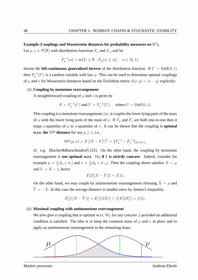
48 CHAPTER 1. MARKOV CHAINS & STOCHASTIC STABILITY
Example (Couplings and Wasserstein distances for probability measures onR1).
Let µ, ν ∈ P(R) with distribution functionsFµ andFν , and let
F−1µ (u) = infc ∈ R : Fµ(c) ≥ u, u ∈ (0, 1),
denote theleft-continuous generalized inverseof the distribution function. IfU ∼ Unif(0, 1)
thenF−1µ (U) is a random variable with lawµ. This can be used to determine optimal couplings
of µ andν for Wasserstein distances based on the Euclidean metricd(x, y) = |x− y| explicitly:
(i) Coupling by monotone rearrangement
A straightforward coupling ofµ andν is given by
X = F−1µ (U) andY = F−1
ν (U), whereU ∼ Unif(0, 1).
This coupling is a monotone rearrangement, i.e., it couplesthe lower lying parts of the mass
of µ with the lower lying parts of the mass ofν. If Fµ andFν are both one-to-one then it
mapsu-quantiles ofµ to u-quantiles ofν. It can be shown that the coupling isoptimal
w.r.t. the Wp distancefor anyp ≥ 1, i.e.,
Wp(µ, ν) = E [|X − Y |p] 1p = ‖F−1µ − F−1
ν ‖Lp(0,1),
cf. e.g. [Rachev&Rueschendorf] [25]. On the other hand, the coupling by monotone
rearrangement isnot optimal w.r.t. Wf if f is strictly concave. Indeed, consider for
exampleµ = 12(δ0 + δ1) andν = 1
2(δ0 + δ−1). Then the coupling above satisfiesX ∼ µ
andY = X − 1, hence
E[f(|X − Y |)] = f(1).
On the other hand, we may couple by antimonotone rearrangement choosingX ∼ µ and
Y = −X. In this case the average distance is smaller since by Jensen’s inequality,
E[f(|X − Y |)] = E[f(2X)] < f(E[2X]) = f(1).
(ii) Maximal coupling with antimonotone rearrangement
We now give a coupling that is optimal w.r.t.Wf for any concavef provided an additional
condition is satisfied. The idea is to keep the common mass ofµ andν in place and to
apply an antimonotone rearrangement to the remaining mass:
µ ν
Markov processes Andreas Eberle
1.5. COUPLINGS AND TRANSPORTATION METRICS 49
Suppose thatS = S+∪S− andµ−ν = (µ−ν)+−(µ−ν)− is a Hahn-Jordan decomposition
of the finite signed measureµ− ν into a difference of positive measures such that
(µ− ν)+(A∩S−) = 0 and(µ− ν)−(A∩S+) = 0 for anyA ∈ B, cf. also Section 1.6. Let
µ ∧ ν = µ− (µ− ν)+ = ν − (µ− ν)−.
If p = (µ∧ ν)(S) is the total shared mass of the measuresµ andν then we can writeµ and
ν as mixtures
µ = (µ ∧ ν) + (µ− ν)+ = pα + (1− p)β,
ν = (µ ∧ ν) + (µ− ν)− = pα + (1− p)γ
of probability measuresα, β andγ. Hence a coupling(X, Y ) of µ andν as described above
is given by setting
(X, Y ) =
(F−1
α (U), F−1α (U)) if B = 1,
(F−1β (U), F−1
γ (1− U))
if B = 0,
with independent random variablesB ∼Bernoulli(p) andU ∼Unif(0, 1). It can be shown
that ifS+ andS− are intervals then(X, Y ) is an optimal coupling w.r.t.Wf for any concave
f , cf. [McCann:Exact solution to the transportation problem on the line] [22].
In contrast to the one-dimensional case it is not easy to describe optimal couplings onRd for
d > 1 explicitly. On the other hand, the existence of optimal couplings holds on an arbitrary
polish spaceS by Prokhorov’s Theorem:
Theorem 1.17(Existence of optimal couplings). For anyµ, ν ∈ P(S) and anyp ∈ [1,∞) there
exists a couplingγ ∈ Π(µ, ν) such that
Wp(µ, ν)p =
ˆ
d(x, y)pγ(dxdy).
Proof: Let I(γ) :=´
d(x, y)pγ(dxdy). By definition of Wp(µ, ν) there exists a minimizing
sequence(γn) in Π(µ, ν) such that
I(γn) → Wp(µ, ν)p asn→ ∞.
Moreover, such a sequence is automatically tight inP(S × S). Indeed, letε > 0 be given. Then,
sinceS is a polish space, there exists a compact setK ⊂ S such that
µ(S \K) <ε
2, ν(S \K) <
ε
2,
University of Bonn Winter term 2014/2015
50 CHAPTER 1. MARKOV CHAINS & STOCHASTIC STABILITY
and hence for anyn ∈ N,
γn ((x, y) /∈ K ×K) ≤ γn(x /∈ K) + γn(y /∈ K)
= µ(S \K) + ν(S \K) < ε.
Prokhorov’s Theorem now implies that there is a subsequence(γnk) that converges weakly to a
limit γ ∈ P(S × S). It is straightforward to verify thatγ is again a coupling ofµ andν, and,
sinced(x, y)p is (lower semi-)continuous,
I(γ) =
ˆ
d(x, y)pγ(dxdy) ≤ lim infk→∞
ˆ
d(x, y)pγnk(dxdy) = Wp(µ, ν)p
by the portemanteau Theorem.
Lemma 1.18(Triangle inequality ). Wp is a metric onPp(S).
Proof: Let µ, ν, ∈ Pp(S). We prove the triangle inequality
Wp(µ, ) ≤ Wp(µ, ν) +Wp(ν, ). (1.5.2)
The other properties of a metric can be verified easily. To prove (1.5.2) letγ andγ be couplings
of µ andν, ν and respectively. We show
Wp(µ, ) ≤(ˆ
d(x, y)pγ(dxdy)
) 1p
+
(ˆ
d(y, z)pγ(dydz)
) 1p
. (1.5.3)
The claim then follows by taking the infimum over allγ ∈ Π(µ, ν) andγ ∈ Π(ν, ). SinceS is a
polish space we can disintegrate
γ(dxdy) = µ(dx)p(x, dy) and γ(dydz) = ν(dy)p(y, dz)
wherep andp are regular versions of conditional distributions of the first component w.r.t.γ, γ
given the second component. The disintegration enables us to “glue” the couplingsγ andγ to a
joint coupling
γ(dxdydz) := µ(dx)p(x, dy)p(y, dz)
of the measuresµ, ν and such that underγ,
(x, y) ∼ γ and (y, z) ∼ γ.
Therefore, by the triangle inequality for theLp norm, we obtain
Wp(µ, ) ≤(ˆ
d(x, z)pγ(dxdydz)
) 1p
≤(ˆ
d(x, y)pγ(dxdydz)
) 1p
+
(ˆ
d(y, z)pγ(dxdydz)
) 1p
=
(ˆ
d(x, y)pγ(dxdy)
) 1p
+
(ˆ
d(y, z)pγ(dydz)
) 1p
.
Markov processes Andreas Eberle
1.5. COUPLINGS AND TRANSPORTATION METRICS 51
Exercise(Couplings inRd). LetW : Ω → Rd be a random variable on(Ω,A, P ) with
W ∼ −W , and letµa denote the law ofa+W .
a) (Synchronous coupling) LetX = a+W andY = b+W for a, b ∈ Rd. Show that
W2(µa, µb) = |a− b| = E(|X − Y |2)1/2,
i.e.,(X, Y ) is an optimal coupling w.r.t.W2.
b) (Reflection coupling) LetY = W + b whereW ≡ W − 2e ·W e with e = a−b|a−b| . Prove that
(X, Y ) is also a coupling ofµa andµb, and if |W | ≤ |a−b|2
a.s. then
E(f(|X − Y |
)≤ f(|a− b|) = E (f(|X − Y |))
for any concave, increasing functionf : R+ → R+ such thatf(0) = 0.
1.5.2 Kantorovich-Rubinstein duality
TheLipschitz norm of a functiong : S → R is defined by
‖g‖Lip = supx 6=y
|g(x)− g(y)|d(x, y)
.
Bounds in Wasserstein distances can be used to estimate differences of integrals of Lipschitz
continuous functions w.r.t. different probability measures. Indeed, one even has:
Theorem 1.19(Kantorovich-Rubinstein duality ). For anyµ, ν ∈ P(S),
W1(µ, ν) = sup‖g‖Lip≤1
(ˆ
gdµ−ˆ
gdν
). (1.5.4)
Remark. There is a corresponding dual description ofWp for p > 1 but it takes a more compli-
cated form, cf. [Villani:OT-old&new] [37].
Proof: We only prove the easy “≥” part. For different proofs of the converse inequality see
Rachev and Rueschendorf [25], Villani1 [38], Villani2 [37] and Mufa Chen [4]. For instance one
can approximateµ andν by finite convex combinations of Dirac measures for which (1.5.4) is a
University of Bonn Winter term 2014/2015
52 CHAPTER 1. MARKOV CHAINS & STOCHASTIC STABILITY
consequence of the standard duality principle of linear programming, cf. Chen [4].
To prove “≥” let µ, ν ∈ P(S) andg ∈ C(S). If γ is a coupling ofµ andν thenˆ
gdµ−ˆ
gdν =
ˆ
(g(x)− g(y))γ(dxdy)
≤ ‖g‖Lip
ˆ
d(x, y)γ(dxdy).
Hence, by taking the infimum overγ ∈ Π(µ, ν), we obtainˆ
gdµ−ˆ
gdν ≤ ‖g‖LipW1(µ, ν).
As a consequence of the “≥” part of (1.5.4), we see that if(µn)n∈N is a sequence of probability
measures such thatW1(µn, µ) → 0 then´
gdµn →´
gdµ for any Lipschitz continuous func-
tion g : S → R, and henceµn → µ weakly. The following more general statement connects
convergence in Wasserstein distances and weak convergence:
Theorem 1.20(Wp convergence and weak convergence). Letp ∈ [1,∞).
1) The metric space(Pp(S),Wp) is complete and separable.
2) A sequence(µn) in Pp(S) converges to a limitµ w.r.t. theWp distance if and only ifˆ
gdµn →ˆ
gdµ for anyg ∈ C(S) satisfyingg(x) ≤ C · (1 + d(x, xo)p)
for a finite constantC and somex0 ∈ S.
Among other things, the proof relies on Prokhorov’s Theorem- we refer to [Villani:OT-old&new]
[37].
1.5.3 Contraction coefficients
Let p(x, dy) be a transition kernel on(S,B) and fixq ∈ [1,∞). We will be mainly interested in
the caseq = 1.
Definition (Wasserstein contraction coefficient of a transition kernel). The globalcontraction
coefficientof p w.r.t. the distanceWq is defined as
αq(p) = sup
Wq(µp, νp)
Wq(µ, ν): µ, ν ∈ Pq(S)s.t.µ 6= ν
.
Markov processes Andreas Eberle
1.5. COUPLINGS AND TRANSPORTATION METRICS 53
In other words,αq(p) is the Lipschitz norm of the mapµ 7→ µp w.r.t. theWq distance. By
applying the Banach fixed point theorem, we obtain:
Theorem 1.21(Geometric ergodicity for Wasserstein contractions). If αq(p) < 1 then there
exists a unique invariant probability measureµ of p in Pq(S). Moreover, for any initial distribu-
tion ν ∈ Pq(S), νpn converges toµ with a geometric rate:
Wq(νpn, µ) ≤ αq(p)nW q(ν, µ).
Proof: The Banach fixed point theorem can be applied by Theorem 1.20.
The assumptionαq(p) < 1 seems restrictive. However, one should bear in mind that theunder-
lying metric onS can be chosen adequately. In particular, in applications itis often possible to
find a concave functionf such thatµ 7→ µp is a contraction w.r.t. theW1 distance based on the
modified metricf d.
The next lemma is crucial for boundingαq(p) in applications:
Lemma 1.22(Bounds for contraction coefficients, Path coupling). 1) Suppose that the tran-
sition kernelp(x, dy) is Feller. Then
α(p) = supx 6=y
Wq (p(x, ·), p(y, ·))d(x, y)
. (1.5.5)
2) Moreover, suppose thatS is a geodesic graphwith edge setE in the sense that for any
x, y ∈ S there exists a pathx0 = x, x1, x2, . . . , xn−1, xn = y from x to y such that
xi−1, xi ∈ E for i = 1, . . . , n andd(x, y) =n∑
i=1
d(xi−1, xi). Then
α(p) = supx,y∈E
W (p(x, ·), p(y, ·))d(x, y)
. (1.5.6)
The application of the second assertion of the lemma to proveupper bounds forαq(p) is known
as thepath coupling methodof Bubley and Dyer.
Proof: 1) Letβ := supx 6=y
Wq(p(x,·),p(y,·))d(x,y)
. We have to show that
Wq(µp, νp) ≤ βWq(µ, ν) (1.5.7)
University of Bonn Winter term 2014/2015
54 CHAPTER 1. MARKOV CHAINS & STOCHASTIC STABILITY
holds for arbitrary probability measuresµ, ν ∈ P(S). By definition ofβ and since
Wq(δx, δy) = d(x, y), (1.5.7) is satisfied ifµ andν are Dirac measures.
Next suppose that
µ =∑
x∈Cµ(x)δx and ν =
∑
x∈Cν(x)δy
are convex combinations of Dirac measures, whereC ⊂ S is a countable subset. Then for
anyx, y ∈ C, we can choose a couplingγxy of δxp andδyp such that
(ˆ
d(x′, y′)qγxy(dx′dy′)
) 1q
= Wq(δxp, δyp) ≤ βd(x, y). (1.5.8)
Let ξ(dxdy) be an arbitrary coupling ofµ andν. Then a couplingγ(dx′dy′) of µp andνp
is given by
γ :=
ˆ
γxyξ(dxdy),
and therefore, by (1.5.8),
Wq(µp, νp) ≤(ˆ
d(x′, y′)qγ(dx′dy′)
) 1q
=
(ˆ ˆ
d(x′, y′)qγxy(dx′dy′)ξ(dxdy)
) 1q
≤ β
(ˆ
d(x, y)qξ(dxdy)
) 1q
.
By taking the infimum over all couplingsξ ∈ Π(µ, ν), we see thatµ andν satisfy (1.5.7).
Finally, to show that (1.5.7) holds for arbitraryµ, ν ∈ P(S), note that sinceS is sepa-
rable, there is a countable dense subsetC, and the convex combinations of Dirac measures
based inC are dense inWq. Henceµ andν areWq limits of corresponding convex com-
binationsµn andνn (n ∈ N). By the Feller property, the sequenceµnp andνnp converge
weakly toµp, νp respectively. Hence
Wq(µp, νp) ≤ lim infWq(µnp, νnp)
≤ β lim infWq(µn, νn) = βWq(µ, ν).
2) Let β := sup(x,y)∈E
Wq(p(x,·),p(y,·))d(x,y)
. We show that
Wq(p(x, ·), p(y, ·)) ≤ βd(x, y)
Markov processes Andreas Eberle
1.5. COUPLINGS AND TRANSPORTATION METRICS 55
holds for arbitraryx, y ∈ S. Indeed, letx0 = x, x1, x2, . . . , xn = y be a geodesic fromx
to y such that(xi−1, xi) ∈ E for i = 1, . . . , n. Then by the triangle inequality for theWq
distance,
Wq(p(x, ·), p(y, ·)) ≤n∑
i=1
Wq(p(xi−1, ·), p(xi, ·))
≤ βn∑
i=1
d(xi−1, xi) = βd(x, y),
where we have used in the last equality thatx0, . . . , xn is a geodesic.
Exercise.Letp be a transition kernel onS×S such thatp((x, y), dx′dy′) is a coupling ofp(x, dx′)
andp(y, dy′) for anyx, y ∈ S. Prove that if there exists a distance functiond : S × S → [0,∞)
and a constantα ∈ (0, 1) such that
pd ≤ αd,
then there is a unique invariant probability measureµ of p, and
W1d (νp
n, µ) ≤ αnW1d (ν, µ) for anyν ∈ P1(S).
1.5.4 Glauber dynamics, Gibbs sampler
Let µ be a probability measure on a product space
S = T V = η : V → T.
We assume thatV is a finite set (for example a finite graph) andT is a polish space (e.g.T = Rd).
Depending on the model considered the elements inT are called types, states, spins, colors etc.,
whereas we call the elements ofS configurations. There is a natural transition mechanism onS
that leads to a Markov chain which is reversible w.r.t.µ. The transition step from a configuration
ξ ∈ S to the next configurationξ′ is given in the following way:
• Choose an elementx ∈ V uniformly at random
• Setξ′(y) = ξ(y) for anyy 6= x, and sampleξ′(x) from the conditional distribution w.r.t.
µ(dy) of η(x) given thatη(y) = ξ(y) for anyy 6= x.
To make this precise, we fix a regular versionµ(dη|η = ξ onV \ x) of the conditional proba-
bility given (η(y))y∈V \x, and we define the transition kernelp by
p =1
|V |∑
x∈Vpx, where
University of Bonn Winter term 2014/2015
56 CHAPTER 1. MARKOV CHAINS & STOCHASTIC STABILITY
px(ξ, dξ′) = µ (dξ′|ξ′ = ξ onV \ x) .
Definition. A time-homogeneous Markov chain with transition kernelp is calledGlauber dy-
namicsor random scan Gibbs samplerwith stationary distributionµ.
Thatµ is indeed invariant w.r.t.p is shown in the next lemma:
Lemma 1.23.The transition kernelspx (x ∈ V ) andp satisfy the detailed balance conditions
µ(dξ)px(ξ, dξ′) = µ(dξ′)px(ξ
′, dξ),
µ(dξ)p(ξ, dξ′) = µ(dξ′)p(ξ′, dξ).
In particular,µ is a stationary distribution forp.
Proof: Let x ∈ V , and letη(x) := (η(y))y 6=x denote the configuration restricted toV \ x.
Disintegration of the measureµ into the lawµx of η(x) and the conditional lawµx(·|η(x)) of
η(x) given η(x) yields
µ (dξ) px (ξ, dξ′) = µx
(dξ(x)
)µx
(dξ(x)|ξ(x)
)δξ(x)
(dξ′(x)
)µx
(dξ′(x)|ξ(x)
)
= µx
(dξ′(x)
)µx
(dξ(x)|ξ′(x)
)δξ′(x)
(dξ(x)
)µx
(dξ′(x)|ξ′(x)
)
= µ (dξ′) px (ξ′, dξ) .
Hence the detailed balance condition is satisfied w.r.t.px for anyx ∈ V , and, by averaging over
x, also w.r.t.p.
Examples. In the following examples we assume thatV is the vertex set of a finite graph with
edge setE.
1) Random colourings. HereT is a finite set (the set of possible colours of a vertex), and
µ is the uniform distribution on all admissible colourings ofthe vertices inV such that no
two neighbouring vertices have the same colour:
µ = Unif(η ∈ T V : η(x) 6= η(y) ∀(x, y) ∈ E
).
The Gibbs sampler selects in each step a vertex at random and changes its colour randomly
to one of the colours that are different from all colours of neighbouring vertices.
2) Hard core model. HereT = 0, 1 whereη(x) = 1 stands for the presence of a particle
at the vertexx. The hard core model with fugacityλ ∈ R+ is the probability measureµλ
on0, 1V satisfying
µλ(η) =1Zλλ
∑
x∈Vη(v)
if η(x)η(y) = 0 for any(x, y) ∈ E,
Markov processes Andreas Eberle
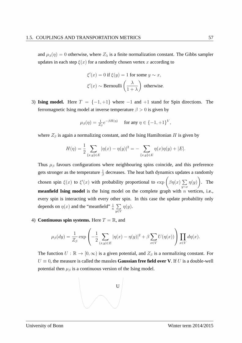
1.5. COUPLINGS AND TRANSPORTATION METRICS 57
andµλ(η) = 0 otherwise, whereZλ is a finite normalization constant. The Gibbs sampler
updates in each stepξ(x) for a randomly chosen vertexx according to
ξ′(x) = 0 if ξ(y) = 1 for somey ∼ x,
ξ′(x) ∼ Bernoulli
(λ
1 + λ
)otherwise.
3) Ising model. HereT = −1,+1 where−1 and+1 stand for Spin directions. The
ferromagnetic Ising model at inverse temperatureβ > 0 is given by
µβ(η) =1Zβe−βH(η) for anyη ∈ −1,+1V ,
whereZβ is again a normalizing constant, and the Ising HamiltonianH is given by
H(η) =1
2
∑
x,y∈E|η(x)− η(y)|2 = −
∑
x,y∈Eη(x)η(y) + |E|.
Thusµβ favours configurations where neighbouring spins coincide,and this preference
gets stronger as the temperature1β
decreases. The heat bath dynamics updates a randomly
chosen spinξ(x) to ξ′(x) with probability proportional toexp
(βη(x)
∑y∼x
η(y)
). The
meanfield Ising model is the Ising model on the complete graph withn vertices, i.e.,
every spin is interacting with every other spin. In this casethe update probability only
depends onη(x) and the “meanfield”1n
∑y∈V
η(y).
4) Continuous spin systems.HereT = R, and
µβ(dy) =1
Zβ
exp
−1
2
∑
(x,y)∈E|η(x)− η(y)|2 + β
∑
x∈VU(η(x))
∏
x∈Vdη(x).
The functionU : R → [0,∞) is a given potential, andZβ is a normalizing constant. For
U ≡ 0, the measure is called the masslesGaussian free field over V. If U is a double-well
potential thenµβ is a continuous version of the Ising model.
U
University of Bonn Winter term 2014/2015
58 CHAPTER 1. MARKOV CHAINS & STOCHASTIC STABILITY
5) Bayesian posterior distributions. Gibbs samplers are applied frequently to sample from
posterior distributions in Bayesian statistical models. For instance in a typical hierarchi-
cal Bayes model one assumes that the data are realizations of conditionally independent
random variablesYij (i = 1, . . . , k, j = 1, . . . ,mi) with conditional laws
Yij|(θ1, . . . , θk, λe) ∼ N (θi, λ−1e ).
The parametersθ1, . . . , θk andλe are again assumed to be conditionally independent ran-
dom variables with
θi|(µ, λθ) ∼ N (µ, λ−1θ ) andλe|(µ, λθ) ∼ Γ(a2, b2).
Finally,µ andλθ are independent with
µ ∼ N (m, v) andλθ ∼ Γ(a1, b1)
wherea1, b1, a2, b2 ∈ R+ andv ∈ R are given constants, cf. [Jones] [13]. The posterior
distributionµ of (θ1, . . . , θk, µ, λe, λθ) onRk+3 given observationsYij = yij is then given
by Bayes’ formula. Although the density is explicitly up to a normalizing constant involv-
ing a possibly high-dimensional integral, it is not clear how to generate exact samples from
µ and how to compute expectation values w.r.t.µ.
On the other hand, it is not difficult to see that all the conditional distributions w.r.t.µ of
one of the parametersθ1, . . . , θk, µ, λe, λθ given all the other parameters are either normal
or Gamma distributions with parameters depending on the observed data. Therefore, it is
easy to run a Gibbs sampler w.r.t.µ on a computer. If this Markov chain converges suffi-
ciently rapidly to its stationary distribution then its values after a sufficiently large number
of steps can be used as approximate samples fromµ, and longtime averages of the values of
a function applied to the Markov chain provide estimators for the integral of this function.
It is then an obvious question for how many steps the Gibbs sampler has to be run to ob-
tain sufficiently good approximations, cf. [Roberts&Rosenthal:Markov chains and MCMC
algorithms] [30].
Returning to the general setup on the product spaceT V , we fix a metric on T , and we denote
by d the correspondingl1 metric on the configuration spaceT V , i.e.,
d(ξ, η) =∑
x∈V (ξ(x), η(x)) , ξ, η ∈ T V .
A frequent choice is (s, t) = 1s 6=t. In this case,
d(ξ, η) = |x ∈ V : ξ(x) 6= η(x)|
is called theHamming distanceof ξ andη.
Markov processes Andreas Eberle
1.5. COUPLINGS AND TRANSPORTATION METRICS 59
Lemma 1.24.Letn = |V |. Then for the Gibbs sampler,
W1d (p(ξ, ·), p(η, ·)) ≤
(1− 1
n
)d(ξ, η) +
1
n
∑
x∈VW1
(µx(·|ξ), µx(·|η))
for anyξ, η ∈ T V .
Proof: Let γx for x ∈ V be optimal couplings w.r.t.W1 of the conditional measuresµx(·|ξ) and
µx(·|η). Then we can construct a coupling ofp(ξ, dξ′) andp(η, dη′) in the following way:
• DrawU ∼ Unif(V ).
• GivenU , choose(ξ′(U), η′(U)) ∼ γU , and setξ′(x) = ξ(x) andη′(x) = η(x) for any
x 6= U .
For this coupling we obtain:
E[d(ξ′, η′)] =∑
x∈VE[(ξ′(x), η′(x))]
= d(ξ, η) + E [(ξ′(U), η′(U))− (ξ(U), η(U))]
= d(ξ, η) +1
n
∑
x∈V
(ˆ
(s, t)γx(dsdt)− (ξ(x), η(x))
)
=
(1− 1
n
)d(ξ, η) +
1
n
∑
x∈VW1
(µx(·|ξ), µx(·|η)) .
Here we have used in the last step the optimality of the coupling γx. The claim follows since
W1d (p(x, ·), p(y, ·)) ≤ E[d(ξ′, η′)].
The lemma shows that we obtain contractivity w.r.t.W1d if the conditional distributions atx ∈ V
do not depend too strongly on the values of the configuration at other vertices:
Theorem 1.25(Geometric ergodicity of the Gibbs sampler for weak interactions).
1) Suppose that there exists a constantc ∈ (0, 1) such that
∑
x∈VW1
(µx(·|ξ), µx(·|η)) ≤ cd(ξ, η) for anyξ, η ∈ T V . (1.5.9)
Then
W1d (νp
t, µ) ≤ α(p)tW1d (ν, µ) for anyν ∈ P(T V ) andt ∈ Z+, (1.5.10)
whereα(p) ≤ exp(−1−c
n
).
University of Bonn Winter term 2014/2015
60 CHAPTER 1. MARKOV CHAINS & STOCHASTIC STABILITY
2) If T is a graph and is geodesic then it suffices to verify(1.5.9)for neighbouring configu-
rationsξ, η ∈ T V such thatξ = η onV \ x for somex ∈ V andξ(x) ∼ η(x).
Proof: 1) If (1.5.9) holds then by Lemma 1.24,
Wd (p(ξ, ·), p(η, ·)) ≤(1− 1− c
n
)d(ξ, η) for anyξ, η ∈ T V .
Hence (1.5.10) holds withα(p) = 1− 1−cn
≤ exp(−1−c
n
).
2) If (T, ) is a geodesic graph andd is the l1 distance based on then (T V , d) is again a
geodesic graph. Indeed, a geodesic path between two configurationsξ andη w.r.t. thel1
distance is given by changing one component after the other along a geodesic path onT .
Therefore, the claim follows from the path coupling lemma 1.22.
The results in Theorem 1.25 can be applied to many basic models including random colourings,
hardcore models and meanfield Ising models at low temperature.
Example (Random colourings). Suppose thatV is a regular graph of degree∆. ThenT V is
geodesic w.r.t. the Hamming distanced. Suppose thatξ andη are admissible random colourings
such thatd(ξ, η) = 1, and lety ∈ V be the unique vertex such thatξ(y) 6= η(y). Then
µx(·|ξ) = µx(·|η) for x = y and for anyx 6∼ y.
Moreover, forx ∼ y and(s, t) = 1s 6=t we have
W1 (µx(·|ξ), µx(·|η)) ≤
1
|T | −∆
since there are at least|T | − ∆ possible colours available, and the possible colours atx givenξ
respectivelyη onV \ x differ only in one colour. Hence
∑
x∈VW1
(µx(·|ξ), µx(·|η)) ≤∆
|T | −∆d(ξ, η),
and therefore, (1.5.10) holds with
α(p) ≤ exp
(−(1− ∆
|T | −∆
)· 1n
), and hence
α(p)t ≤ exp
(−|T | − 2∆
|T | −∆· tn
).
Markov processes Andreas Eberle
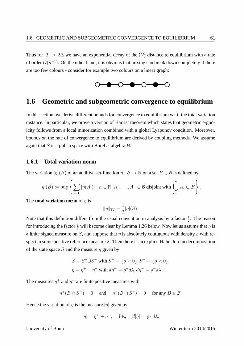
1.6. GEOMETRIC AND SUBGEOMETRIC CONVERGENCE TO EQUILIBRIUM 61
Thus for|T | > 2∆ we have an exponential decay of theW1d distance to equilibrium with a rate
of orderO(n−1). On the other hand, it is obvious that mixing can break down completely if there
are too few colours - consider for example two colours on a linear graph:
bC b bC b bC b bC
1.6 Geometric and subgeometric convergence to equilibrium
In this section, we derive different bounds for convergenceto equilibrium w.r.t. the total variation
distance. In particular, we prove a version of Harris’ theorem which states that geometric ergod-
icity follows from a local minorization combined with a global Lyapunov condition. Moreover,
bounds on the rate of convergence to equilibrium are derivedby coupling methods. We assume
again thatS is a polish space with Borelσ-algebraB.
1.6.1 Total variation norm
The variation|η|(B) of an additive set-functionη : B → R on a setB ∈ B is defined by
|η|(B) := sup
n∑
i=1
|η(Ai)| : n ∈ N, A1, . . . , An ∈ B disjoint withn⋃
i=1
Ai ⊂ B
.
Thetotal variation norm of η is
‖η‖TV =1
2|η|(S).
Note that this definition differs from the usual convention in analysis by a factor12. The reason
for introducing the factor12
will become clear by Lemma 1.26 below. Now let us assume thatη is
a finite signed measure onS, and suppose thatη is absolutely continuous with densitywith re-
spect to some positive reference measureλ. Then there is an explicit Hahn-Jordan decomposition
of the state spaceS and the measureη given by
S = S+∪S− with S+ = ≥ 0, S− = < 0,η = η+ − η− with dη+ = +dλ, dη− = −dλ.
The measuresη+ andη− are finite positive measures with
η+(B ∩ S−) = 0 and η−(B ∩ S+) = 0 for anyB ∈ B.
Hence the variation ofη is the measure|η| given by
|η| = η+ + η−, i.e., d|η| = · dλ.
University of Bonn Winter term 2014/2015
62 CHAPTER 1. MARKOV CHAINS & STOCHASTIC STABILITY
In particular, the total variation norm ofη is theL1 norm of:
‖η‖TV =
ˆ
||dx = ‖‖L1(λ). (1.6.1)
Lemma 1.26 (Equivalent descriptions of the total variation norm). Let µ, ν ∈ P(S) and
λ ∈ M+(S) such thatµ and ν are both absolutely continuous w.r.t.λ. Then the following
identities hold:
‖µ− ν‖TV = (µ− ν)+(S) = (µ− ν)−(S) = 1− (µ ∧ ν)(S)
=
∥∥∥∥dµ
dλ− dν
dλ
∥∥∥∥L1(λ)
=1
2sup |µ(f)− ν(f)| : f ∈ Fb(S) s.t.‖f‖sup ≤ 1 (1.6.2)
= inf P [X 6= Y ] : X ∼ µ, Y ∼ ν (1.6.3)
In particular, ‖µ− ν‖TV ∈ [0, 1].
Remarks. 1) The last identity shows that the total variation distanceof µ andν is the Kan-
torovich distanceW1d (µ, ν) based on the trivial metricd(x, y) = 1x 6=y onS.
2) The assumptionµ, ν << λ can always be satisfied by choosingλ appropriately. For
example, we may chooseλ = µ+ ν.
Proof: Sinceµ andν are both probability measures,
(µ− ν)(S) = µ(S)− ν(S) = 0.
Hence(µ− ν)+(S) = (µ− ν)−(S), and
‖µ− ν‖TV =1
2|µ− ν|(S) = (µ− ν)+(S) = µ(S)− (µ ∧ ν)(S) = (µ− ν)−(S).
The identity‖µ − ν‖TV =∥∥dµdλ
− dνdλ
∥∥L1(λ)
holds by (1.6.1). Moreover, forf ∈ Fb(S) with
‖f‖sup ≤ 1,
|µ(f)− ν(f)| ≤ |(µ− ν)+(f)|+ |(µ− ν)−(f)|≤ (µ− ν)+(S) + (µ− ν)−(S) = 2‖µ− ν‖TV
with identity forf = 1S+ − 1S− . This proves the representation (1.6.2) of‖µ− ν‖TV.
Finally, to prove (1.6.3) note that if(X, Y ) is a coupling ofµ andν, then
|µ(f)− ν(f)| = |E[f(X)− f(Y )]| ≤ 2P [X 6= Y ]
Markov processes Andreas Eberle
1.6. GEOMETRIC AND SUBGEOMETRIC CONVERGENCE TO EQUILIBRIUM 63
holds for any bounded measurablef with ‖f‖sup ≤ 1. Hence by (1.6.2),
‖µ− ν‖TV ≤ infX∼µ
Y∼ν
P [X 6= Y ].
To show the converse inequality we choose a coupling(X, Y ) that maximizes the probability that
X andY agree. The maximal coupling can be constructed by noting that
µ = (µ ∧ ν) + (µ− ν)+ = pα + (1− p)β, (1.6.4)
ν = (µ ∧ ν) + (µ− ν)− = pα + (1− p)γ (1.6.5)
with p = (µ ∧ ν)(S) and probability measuresα, β, γ ∈ P(S). We choose independent random
variablesU ∼ α, V ∼ β,W ∼ γ andZ ∼ Bernoulli(p), and we define
(X, Y ) =
(U,U) onZ = 1,(V,W ) onZ = 0.
Then by (1.6.4) and (1.6.5),(X, Y ) ∈ Π(µ, ν) and
P [X 6= Y ] ≤ P [Z = 0] = 1− p = 1− (µ ∧ ν)(S) = ‖µ− ν‖TV.
Remark. The last equation can also be seen as a special case of the Kantorovich-Rubinstein
duality formula.
1.6.2 Geometric ergodicity
Let p be a transition kernel on(S,B). We define thelocal contraction coefficientα(p,K) of p
on a setK ⊂ S w.r.t. the total variation distance by
α(p,K) = supx,y∈K
‖p(x, ·)− p(y, ·)‖TV = supx,y∈K
x 6=y
‖δxp− δyp‖TV
‖δx − δy‖TV. (1.6.6)
Note that in contrast to more general Wasserstein contraction coefficients, we always have
α(p,K) ≤ 1.
Moreover,α(p,K) ≤ 1 − ε holds for ε > 0 if p satisfies the followinglocal minorization
condition: There exists a probability measureν onS such that
p(x,B) ≥ εν(B) for anyx ∈ K andB ∈ B. (1.6.7)
University of Bonn Winter term 2014/2015
64 CHAPTER 1. MARKOV CHAINS & STOCHASTIC STABILITY
Doeblin’s classical theorem states that ifα(pn, S) < 1 for somen ∈ N then there exists a unique
stationary distributionµ of p, and uniform ergodicity holds in the following sense:
supx∈S
‖pt(x, ·)− µ‖TV → 0 ast→ ∞. (1.6.8)
Exercise(Doeblin’s Theorem). Prove that (1.6.8) holds ifα(pn, S) < 1 for somen ∈ N.
If the state space is infinite, a global contraction condition w.r.t. the total variation norm as
assumed in Doeblin’s Theorem can not be expected to hold:
Example (Autoregressive process AR(1)). Suppose that
Xn+1 = αXn +Wn+1, X0 = x
with α ∈ (−1, 1), x ∈ R, and i.i.d. random variablesWn : Ω → R. By induction, one easily
verifies that
Xn = αnx+n−1∑
i=0
αiWn−i ∼ N
(αnx,
1− α2n
1− α2
),
i.e., then-step transition kernel is given by
pn(x, ·) = N
(αnx,
1− α2n
1− α2
), x ∈ S.
As n→ ∞, pn(x, ·) → µ in total variation, where
µ = N
(0,
1
1− α2
)
is the unique stationary distribution. However, the convergence is not uniform inx, since
supx∈R
‖pn(x, ·)− µ‖TV = 1 for anyn ∈ N.
The example demonstrates the need of a weaker notion of convergence to equilibrium than uni-
form ergodicity, and of a weaker assumption than the global minorization condition.
Definition (Geometric ergodicity). A time-homogeneous Markov chain(Xn, Px) with transition
kernelp is calledgeometrically ergodic with stationary distributionµ iff there existγ ∈ (0, 1)
and a non-negative functionM : S → R such that
‖pn(x, ·)− µ‖TV ≤M(x)γn for µ-almost everyx ∈ S.
Harris’ Theorem states that geometric ergodicity is a consequence of alocal minorization con-
dition and a globalLyapunov condition of the following form:
Markov processes Andreas Eberle
1.6. GEOMETRIC AND SUBGEOMETRIC CONVERGENCE TO EQUILIBRIUM 65
(LG) There exist a functionV ∈ F+(S) and constantsλ > 0 andC <∞ such that
LV (x) ≤ C − λV (x) for anyx ∈ S. (1.6.9)
In terms of the transition kernel the condition (LG) states that
pV (x) ≤ C + γV (x) (1.6.10)
whereγ = 1− λ < 1.
Below, we follow the approach of M. Hairer and J. Mattingly to give a simple proof of a quan-
titative version of the Harris Theorem, cf. [Hairer:Convergence of Markov processes,Webpage
M.Hairer] [12]. The key idea is to replace the total variation distance by the Kantorovich distance
Wβ(µ, ν) = infX∼µ
Y∼ν
E[dβ(µ, ν)]
based on a distance function onS of the form
dβ(x, y) = (1 + βV (x) + βV (y)) 1x 6=y
with β > 0. Note that‖µ− ν‖TV ≤ Wβ(µ, ν) with equality forβ = 0.
Theorem 1.27(Quantitative Harris Theorem ). Suppose that there exists a functionV ∈ F+(S)
such that the condition in (LG) is satisfied with constantsC, λ ∈ (0,∞), and
α(p, V ≤ r) < 1 for somer > 2C/λ. (1.6.11)
Then there exists a constantβ ∈ R+ such thatαβ(p) < 1. In particular, there is a unique
stationary distributionµ of p satisfying´
V dµ <∞, and geometric ergodicity holds:
‖pn(x, ·)− µ‖TV ≤ Wβ (pn(x, ·), µ) ≤
(1 + βV (x) + β
ˆ
V dµ
)αβ(p)
n
for anyn ∈ N andx ∈ S.
Remark. There are explicit expressions for the constantsβ andαβ(p).
Proof: Fix x, y ∈ S with x 6= y, and let(X, Y ) be amaximal coupling ofp(x, ·) andp(y, ·)w.r.t. the total variation distance, i.e.,
P [X 6= Y ] = ‖p(x, ·)− p(y, ·)‖TV.
University of Bonn Winter term 2014/2015
66 CHAPTER 1. MARKOV CHAINS & STOCHASTIC STABILITY
Then forβ ≥ 0,
Wβ(p(x, ·), p(y, ·)) ≤ E[dβ(X, Y )]
≤ P [X 6= Y ] + βE[V (X)] + βE[V (Y )]
= ‖p(x, ·)− p(y, ·)‖TV + β(pV )(x) + β(pV )(y)
≤ ‖p(x, ·)− p(y, ·)‖TV + 2Cβ + (1− λ)β(V (x) + V (y)), (1.6.12)
where we have used (1.6.10) in the last step. We now fixr as in (1.6.11), and distinguish cases:
(i) If V (x)+V (y) ≥ r, then the Lyapunov condition ensures contractivity. Indeed, by (1.6.12),
Wβ(p(x, ·), p(y, ·)) ≤ dβ(x, y) + 2Cβ − λβ · (V (x) + V (y)). (1.6.13)
Sincedβ(x, y) = 1 + βV (x) + βV (y), the expression on the right hand side in (1.6.13)
is bounded from above by(1 − δ)dβ(x, y) for some constantδ > 0 provided2Cβ + δ ≤(λ− δ)βr. This condition is satisfied if we choose
δ :=λ− 2C
r
1 + 1βr
=λr − 2C
1 + βrβ,
which is positive sincer > 2C/λ.
(ii) If V (x) + V (y) < r then contractivity follows from (1.6.11). Indeed, (1.6.12) implies that
for ε := min(
1−α(p,V≤r)2
, λ)
,
Wβ(p(x, ·), p(y, ·)) ≤ α(p, V ≤ r) + 2Cβ + (1− λ)β(V (x) + V (y))
≤ (1− ε)dβ(x, y)
providedβ ≤ 1−α(p,V≤r)4C
.
Choosingδ, ε, β > 0 as in (i) and (ii), we obtain
Wβ(p(x, ·), p(y, ·)) ≤ (1−min(δ, ε))dβ(x, y) for anyx, y ∈ S,
i.e., theglobal contraction coefficientαβ(p) w.r.t. Wβ is strictly smaller than one. Hence there
exists a unique stationary distribution
µ ∈ P1β(S) =
µ ∈ P(S) :
ˆ
V dµ <∞, and
Wβ(pn(x, ·), µ) = Wβ (δxp
n, µpn) ≤ αβ(p)nWβ(δx, µ)
= αβ(p)n
(1 + βV (x) + β
ˆ
V dµ
).
Markov processes Andreas Eberle
1.6. GEOMETRIC AND SUBGEOMETRIC CONVERGENCE TO EQUILIBRIUM 67
Remark (Doeblin’s Theorem). If α(p, S) < 1 then by choosingV ≡ 0, we recover Doeblin’s
Theorem:
‖pn(x, ·)− µ‖TV ≤ α(p, S)n → 0 uniformly in x ∈ S.
Example (State space model inRd). Consider the Markov chain with state spaceRd and tran-
sition step
x 7→ x+ b(x) + σ(x)W,
whereb : Rd → Rd andσ : Rd → Rd×d are measurable functions, andW : Ω → Rd is a random
vector withE[W ] = 0 andCov(Wi,Wj) = δij. ChoosingV (x) = |x|2, we obtain
LV (x) = 2x · b(x) + |b(x)|2 + tr(σTσ)(x) ≤ C − λV (x)
for someC, λ ∈ (0,∞) provided
lim sup|x|→∞
x · b(x) + |b(x)|2 + tr(σTσ)(x)
|x|2 < 0.
Since
α(p, V ≤ r) = sup|x|≤√
r
sup|y|≤√
r
∥∥N(x+ b(x), (σσT )(x)
)−N
(y + b(y), (σσT )(y)
)∥∥TV< 1
for anyr ∈ (0,∞), the conditions in Harris’ Theorem are satisfied in this case.
Example (Gibbs Sampler in Bayesian Statistics). For several concrete Bayesian posterior dis-
tributions on moderately high dimensional spaces, Theorem1.27 can be applied to show that the
total variation distance between the law of the Gibbs sampler aftern steps and the stationary target
distribution is small after a feasible number of iterations, cf. e.g. [Roberts&Rosenthal:Markov
chains & MCMC algorithms] [30].
1.6.3 Couplings of Markov chains and convergence rates
On infinite state spaces, convergence to equilibrium may hold only at asubgeometric (i.e.,
slower than exponential) rate. Roughly, subgeometric convergence occurs if the drift is not strong
enough to push the Markov chain rapidly back towards the center of the state space. There are
two possible approaches for proving convergence to equilibrium at subgeometric rates:
a) The Harris’ Theorem can be extended to the subgeometric case provided a Lyapunov con-
dition of the form
LV ≤ C − ϕ V
holds with a concave increasing functionϕ : R+ → R+ satisfyingϕ(0) = 0, cf. [Hairer]
[12] and [Meyn&Tweedie] [23].
University of Bonn Winter term 2014/2015
68 CHAPTER 1. MARKOV CHAINS & STOCHASTIC STABILITY
b) Alternatively, couplings of Markov chains can be applieddirectly to prove both geometric
and subgeometric convergence bounds.
Both approaches eventually lead to similar conditions. We focus now on the second approach.
Definition (Couplings of stochastic processes).
1) A coupling of two stochastic processes(Xn, P ) and (Yn, Q) with state spaceS andT is
given by a process((X, Y ), P
)with state spaceS × T such that
(Xn)n≥0 ∼ (Xn)n≥0 and (Yn)n≥0 ∼ (Yn)n≥0.
2) The coupling is calledMarkovian iff the process(Xn, Yn)n≥0 is a Markov chain on the
product spaceS × T .
Example (Construction of Markovian couplings). A Markovian coupling of two time homo-
geneous Markov chains can be constructed from a coupling of the transition functions. Suppose
thatp andq are transition kernels on measurable spaces(S,B) and(T, C), andp is a transition
kernel on(S × T,B ⊗ C) such thatp ((x, y), dx′dy′) is a coupling of the measuresp(x, dx′) and
p(y, dy′) for anyx ∈ S andy ∈ T . Then for anyx ∈ S andy ∈ T , the canonical Markov chain
((Xn, Yn), Pxy) with transition kernelp and initial distributionδx,y is a Markovian coupling of
Markov chains with transition kernelsp andq and initial distributionsδx andδy. More generally,
((Xn, Yn), Pγ) is a coupling of Markov chains with transition kernelsp, q and initial distributions
µ, ν providedγ is a coupling ofµ andν.
Theorem 1.28(Coupling lemma). Suppose that((Xn, Yn)n≥0, P ) is a Markovian coupling of
Markov chains with transition kernelp and initial distributionsµ andν. Then
‖µpn − νpn‖TV ≤ ‖Law(Xn:∞)− Law(Yn:∞)‖TV ≤ P [T > n],
whereT is thecoupling timedefined by
T = minn ≥ 0 : Xn = Yn.
In particular, ifT <∞ almost surely then
limn→∞
‖Law(Xn:∞)− Law(Yn:∞)‖TV = 0.
Markov processes Andreas Eberle
1.6. GEOMETRIC AND SUBGEOMETRIC CONVERGENCE TO EQUILIBRIUM 69
Proof: 1) We first show that we may assume without loss of generality thatXn = Yn for any
n ≥ T . Indeed, if this is not the case then we can define a modified coupling (Xn, Yn) with
the same coupling timeby setting
Yn :=
Yn for n < T,
Xn for n ≥ T.
The fact that(Xn, Yn) is again a coupling of the same Markov chains follows from the
strong Markov property:T is a stopping time w.r.t. the filtration(Fn) generated by the
process(Xn, Yn), and hence onT < ∞ and under the conditional law givenFT , XT :∞
is a Markov chain with transition kernelp and initial valueYT . Therefore, the conditional
law of
Y0:∞ = (Y1, . . . , YT−1, XT , XT+1, . . . )
givenFT coincides with the conditional law of
Y0:∞ = (Y1, . . . , YT−1, YT , YT+1, . . . )
givenFT , and hence the unconditioned law of(Yn) and(Yn) coincides as well.
2) Now suppose thatXn = Yn for n ≥ T . Then alsoXn:∞ = Yn:∞ for n ≥ T , and thus we
obtain
‖Law(Xn:∞)− Law(Yn:∞)‖TV ≤ P [Xn:∞ 6= Yn:∞] ≤ P [T > n].
If µ is a stationary distribution forp thenµpn = µ and Law(Xn:∞) = Pµ for anyn ≥ 0. Hence
the coupling lemma provides upper bounds for the total variation distance to stationarity. As an
immediate consequence we note:
Corollary 1.29 (Convergence rates by coupling). LetT be the coupling time for a Markovian
coupling of time-homogeneous Markov chains with transitionkernelp and initial distributionsµ
andν. Suppose that
E[ψ(T )] <∞
for some increasing functionψ : Z+ → R+ with limn→∞
ψ(n) = ∞. Then
‖µpn − νpn‖TV = O
(1
ψ(n)
), and even (1.6.14)
∞∑
n=0
(ψ(n+ 1)− ψ(n)) ‖µpn − νpn‖TV <∞. (1.6.15)
University of Bonn Winter term 2014/2015
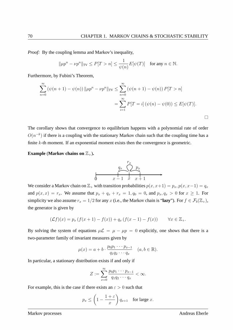
70 CHAPTER 1. MARKOV CHAINS & STOCHASTIC STABILITY
Proof: By the coupling lemma and Markov’s inequality,
‖µpn − νpn‖TV ≤ P [T > n] ≤ 1
ψ(n)E[ψ(T )] for anyn ∈ N.
Furthermore, by Fubini’s Theorem,
∞∑
n=0
(ψ(n+ 1)− ψ(n)) ‖µpn − νpn‖TV ≤∞∑
n=0
(ψ(n+ 1)− ψ(n))P [T > n]
=∞∑
i=1
P [T = i] (ψ(n)− ψ(0)) ≤ E[ψ(T )].
The corollary shows that convergence to equilibrium happens with a polynomial rate of order
O(n−k) if there is a coupling with the stationary Markov chain such that the coupling time has a
finite k-th moment. If an exponential moment exists then the convergence is geometric.
Example (Markov chains onZ+).
0 x− 1 x x+ 1
qx
rxpx
We consider a Markov chain onZ+ with transition probabilitiesp(x, x+1) = px, p(x, x−1) = qx
andp(x, x) = rx. We assume thatpx + qx + rx = 1, q0 = 0, andpx, qx > 0 for x ≥ 1. For
simplicity we also assumerx = 1/2 for anyx (i.e., the Markov chain is “lazy”). For f ∈ Fb(Z+),
the generator is given by
(Lf)(x) = px (f(x+ 1)− f(x)) + qx (f(x− 1)− f(x)) ∀x ∈ Z+.
By solving the system of equationsµL = µ − µp = 0 explicitly, one shows that there is a
two-parameter family of invariant measures given by
µ(x) = a+ b · p0p1 · · · px−1
q1q2 · · · qx(a, b ∈ R).
In particular, a stationary distribution exists if and onlyif
Z :=∞∑
x=0
p0p1 · · · px−1
q1q2 · · · qx<∞.
For example, this is the case if there exists anε > 0 such that
px ≤(1− 1 + ε
x
)qx+1 for largex.
Markov processes Andreas Eberle
1.6. GEOMETRIC AND SUBGEOMETRIC CONVERGENCE TO EQUILIBRIUM 71
Now suppose that a stationary distributionµ exists. To obtain an upper bound on the rate of
convergence toµ, we consider the straightforward Markovian coupling((Xn, Yn), Pxy) of two
chains with transition kernelp determined by the transition step
(x, y) →
(x+ 1, y) with probabilitypx,
(x− 1, y) with probabilityqx,
(x, y + 1) with probabilitypx,
(x, y − 1) with probabilityqx.
Since at each transition step only one of the chains(Xn) and (Yn) is moving one unite, the
processes(Xn) and(Yn) meet before the trajectories cross each other. In particular, if X0 ≥ Y0
then the coupling timeT is bounded from above by the first hitting time
TX0 = minn ≥ 0 : Xn = 0.
Since a stationary distribution exists and the chain is irreducible, all states are positive recurrent.
Hence
E[T ] ≤ E[TX0 ] <∞.
Therefore by Corollary 1.29, the total variation distance from equilibrium isalwaysdecaying at
least of orderO(n−1):
‖pn(x, ·)− µ‖TV = O(n−1),∞∑
n=1
‖pn(x, ·)− µ‖TV <∞.
To prove a stronger decay, one can construct appropriate Lyapunov functions for bounding higher
moments ofT . For instance suppose that
px − qx ∼ −axγ as x→ ∞
for somea > 0 andγ ∈ (−1, 0].
(i) If γ ∈ (−1, 0) then asx→ ∞, the functionV (x) = xn (n ∈ N) satisfies
LV (x) = px ((x+ 1)n − xn) + qx ((x− 1)n − xn) ∼ n(px − qx)xn−1
∼ −naxn−1+γ ≤ −naV (x)1−1−γn .
It can now be shown in a similar way as in the proofs of Theorem 1.6 or Theorem 1.9 that
E[T k] ≤ E[(TX0 )k] <∞ for anyk <
n
1− γ.
University of Bonn Winter term 2014/2015
72 CHAPTER 1. MARKOV CHAINS & STOCHASTIC STABILITY
Sincen can be chosen arbitrarily large, we see that the convergencerate is faster than any
polynomial rate:
‖pn(x, ·)− µ‖TV = O(n−k) for anyk ∈ N.
Indeed, by choosing faster growing Lyapunov functions one can show that the convergence
rate isO(exp (−nβ)) for someβ ∈ (0, 1) depending onγ.
(ii) If γ = 0 then even geometric convergence holds. Indeed, in this case, for largex, the
functionV (x) = eλx satisfies
LV (x) =(px(eλ − 1
)+ qx
(e−λ − 1
))V (x) ≤ −c · V (x)
for some constantc > 0 providedλ > 0 is chosen sufficiently small. Hence geometric
ergodicity follows either by Harris’ Theorem, or, alternatively, by applying Corollary 1.29
with ψ(n) = ecn.
1.7 Mixing times
Let p be a transition kernel on(S,B) with stationary distributionµ. ForK ∈ B andt ≥ 0 let
dTV(t,K) = supx∈K
‖pt(x, ·)− µ‖TV
denote the maximal total variation distance from equilibrium aftert steps of the Markov chain
with transition kernelp and initial distribution concentrated onK.
Definition (Mixing time ). For ε > 0, theε-mixing time of the chain with initial value inK is
defined by
tmix(ε,K) = mint ≥ 0 : d(t,K) ≤ ε.
Moreover, we denote bytmix(ε) the global mixing timetmix(ε, S).
Exercise(Decay of TV-distance to equilibrium).
Prove that for any initial distributionν ∈ P(S), the total variation distance‖νpt − µ‖TV is a
decreasing function int. Hence conclude that
dTV(t,K) ≤ ε for anyt ≥ tmix(ε,K).
An important problem is the dependence of mixing times on parameters such as the dimension
of the underlying state space. In particular, the distinction between “slow” and “rapid ” mixing,
i.e., exponential vs. polynomial increase of the mixing time as a parameter goes to infinity, is
often related to phase transitions.
Markov processes Andreas Eberle
1.7. MIXING TIMES 73
1.7.1 Upper bounds in terms of contraction coefficients
To quantify mixing times note that by the triangle inequality for the TV-distances,
dTV(t, S) ≤ α(pt) ≤ 2dTV(t, S),
whereα denotes the global TV-contraction coefficient.
Example (Random colourings). For the random colouring chain with state spaceT V , we have
shown in the example below Theorem 1.25 that for|T | > 2∆, the contraction coefficientαd w.r.t.
the Hamming distanced(ξ, η) = |x ∈ V : ξ(x) 6= η(x)| satisfies
αd(pt) ≤ αd(p)
t ≤ exp
(−|T | − 2∆
|T | −∆· tn
). (1.7.1)
Here∆ denotes the degree of the regular graphV andn = |V |. Since
1ξ 6=η ≤ d(ξ, η) ≤ n · 1ξ 6=η for anyξ, η ∈ T V ,
we also have
‖ν − µ‖TV ≤ W1d (ν, µ) ≤ n‖ν − µ‖TV for anyν ∈ P(S).
Therefore, by (1.7.1), we obtain
‖pt(ξ, ·)− µ‖TV ≤ nαd(pt) ≤ n exp
(−|T | − 2∆
|T | −∆· tn
)
for anyξ ∈ T V andt ≥ 0. The right-hand side is smaller thanε for t ≥ |T |−∆|T |−2∆
n log(n/ε). Thus
we have shown that
tmix(ε) = O(n log n+ n log ε−1
)for |T | > 2∆.
This is a typical example ofrapid mixing with a total variationcast-off: After a time of order
n log n, the total variation distance to equilibrium decays to an arbitrary small valueε > 0 in a
time window of orderO(n).
Example (Harris Theorem). In the situation of Theorem 1.27, the global distancedTV(t, S) to
equilibrium does not go to0 in general. However, on the level sets of the Lyapunov functionV ,
dTV(t, V ≤ r) ≤(1 + βr + β
ˆ
V dµ
)αβ(p)
t
for any t, r ≥ 0 whereβ is chosen as in the theorem, andαβ is the contraction coefficient w.r.t.
the corresponding distancedβ. Hence
tmix(ε, V ≤ r) ≤ log(1 + βr + β
´
V dµ)+ log(ε−1)
log(αβ(p)−1).
University of Bonn Winter term 2014/2015
74 CHAPTER 1. MARKOV CHAINS & STOCHASTIC STABILITY
1.7.2 Upper bounds by Coupling
We can also apply the coupling lemma to derive upper bounds for mixing times in the following
way:
Corollary 1.30 (Coupling times and mixing times). Suppose that((Xn, Yn), Px,y) is a Marko-
vian coupling of the Markov chains with initial valuex, y ∈ S and transition kernelp for any
x, y ∈ S, and letT = infn ∈ Z+ : Xn = Yn. Then:
1) ‖pn(x, ·)− pn(y, ·)‖TV ≤ Px,y[T > n] for anyx, y ∈ S andn ∈ N.
2) α(pn, K) ≤ supx,y∈K
Px,y[T > n].
Example (Lazy Random Walks). A lazy random walk on a graph is a random walk that stays
in its current position during each step with probability1/2. Lazy random walks are considered
to exclude periodicity effects that may occur due to the timediscretization. By a simple coupling
argument we obtain bounds for total variation distances andmixing times on different graphs:
1) S = Z: Here the transition probabilities of the lazy simple randomwalk arep(x, x+ 1) =
p(x, x − 1) = 1/4, p(x, x) = 1/2, andp(x, y) = 0 otherwise. A Markovian coupling
(Xn, Yn) is given by moving from(x, y) to (x+1, y), (x− 1, y), (x, y+1), (x, y− 1) with
probability 1/2 each. Hence only one of two copies is moving during each step so that
the two random walksXn andYn can not cross each other without meeting at the same
position. The coupling timeT is the hitting time of0 for the processXn − Yn which is a
simple random walk onZ. HenceT <∞ Px,y-almost surely, and
limn→∞
‖pn(x, ·)− pn(y, ·)‖TV = 0 for anyx, y ∈ S.
Nevertheless, a stationary distribution does not exist.
2) S = Z/(mZ): On a discrete circle withm points we can use the analogue coupling for the
lazy random walk. Again,Xn−Yn is a simple random walk onS, andT is the hitting time
of 0. Hence by the Poisson equation,
Ex,y[T ] = ERW(Z)|x−y| [T1,2,...,m−1c ] = |x− y| · (m− |x− y|) ≤ 1
nm2.
Corollary 1.30 and Markov’s inequality now implies that the TV-distance to the uniform
distribution aftern steps is bounded from above by
dTV(n, S) ≤ α(pn) ≤ supx,y
Px,y[T > n] ≤ m2
4n.
Hencetmix(1/4) ≤ m2 which is a rather sharp upper bound.
Markov processes Andreas Eberle
1.7. MIXING TIMES 75
3) S = 0, 1d: The lazy random walk on the hypercube0, 1d coincides with the Gibbs sam-
pler for the uniform distribution. Constructing a coupling similarly as before, the coupling
time T is bounded from above by the first time where each coordinate has been updated
once, i.e., by the number of draws required to collect each ofd coupons by sampling with
replacement. Therefore, forc ≥ 0,
dTV(d log d+ cd) ≤ P [T > d log d+ cd]
≤d∑
k=1
(1− 1
d
)⌈d log d+cd⌉≤ de−
d log d+cdd ≤ e−c,
and hence
tmix(ε) ≤ d log d+ log(ε−1)d.
Conversely the coupon collecting problem also shows that this upper bound is again almost
sharp.
1.7.3 Conductance lower bounds
A simple and powerful way to derive lower bounds for mixing times due to constraints by bottle-
necks is the conductance.
Exercise(Conductance and lower bounds for mixing times). Let p be a transition kernel on
(S,B) with stationary distributionµ. For setsA,B ∈ B with µ(A) > 0, theequilibrium flow
Q(A,B) fromA toB is defined by
Q(A,B) = (µ⊗ p)(A×B) =
ˆ
A
µ(dx) p(x,B),
and theconductanceof A is given by
Φ(A) =Q(A,AC)
µ(A).
Thebottleneck ratio (isoperimetric constant)Φ∗ is defined as
Φ∗ = minA:µ(A)≤1/2
Φ(A).
Let µA(B) = µ(B|A) denote the conditioned measure onA.
a) Show that for anyA ∈ B with µ(A) > 0,
‖µAp− µA‖TV = (µAp)(AC) = Φ(A).
Hint: Prove first that
University of Bonn Winter term 2014/2015

76 CHAPTER 1. MARKOV CHAINS & STOCHASTIC STABILITY
(i) (µAp)(B)− µA(B) ≤ 0 for any measurableB ⊆ A, and
(ii) (µAp)(B)− µA(B) = (µAp)(B) ≥ 0 for any measurableB ⊆ AC .
b) Conclude that
‖µA − µ‖TV ≤ tΦ(A) + ‖µApt − µ‖TV for anyt ∈ Z+.
c) Hence prove the lower bound
tmix
(1
4
)≥ 1
4Φ∗.
Markov processes Andreas Eberle
Chapter 2
Ergodic averages
Suppose that(Xn, Px) is a canonical time-homogeneous Markov chain with transition kernelp.
Recall that the process(Xn, Pµ) with initial distributionµ is stationary, i.e.,
Xn:∞ ∼ X0:∞ for anyn ≥ 0,
if and only if
µ = µp.
A probability measureµ with this property is called astationary (initial) distribution or an
invariant probability measure for the transition kernel p. In this chapter we will prove law
of large number type theorems for ergodic averages of the form
1
n
n−1∑
i=0
f(Xi) →ˆ
fdµ asn→ ∞,
and, more generally,
1
n
n−1∑
i=0
F (Xi, Xi+1, . . . ) →ˆ
FdPµ asn→ ∞
whereµ is a stationary distribution for the transition kernel. At first these limit theorems are de-
rived almost surely or inLp w.r.t. the lawPµ of the Markov chain in stationarity. Indeed, they turn
out to be special cases of more general ergodic theorems for stationary (not necessarily Marko-
vian) stochastic processes. After the derivation of the basic results we will consider extensions to
continuous time, and we will briefly discuss the validity of ergodic theorems for Markov chains
that are not started in stationary. Moreover, we will study the fluctuations of ergodic averages
around their limit both asymptotically and non-asymptotically. As usual,S will denote a polish
space endowed with its Borelσ-algebraB.
77
78 CHAPTER 2. ERGODIC AVERAGES
2.1 Ergodic theorems
Supplementary references for this section are the probability theory textbooks by Breimann
[XXX], Durrett [XXX] and Varadhan [XXX].We first introduce the more general setup of
ergodic theory that includes stationary Markov chains as a special case:
Let (Ω,A, P ) be a probability space, and let
Θ : Ω → Ω
be a measure-preserving measurable map on(Ω,A, P ), i.e.,
P Θ−1 = P.
The main example is the following: Let
Ω = SZ+ , Xn(ω) = ωn, A = σ(Xn : n ∈ Z+),
be the canonical model for a stochastic process with state spaceS. Then the shift transformation
Θ = X1:∞ given by
Θ(ω0, ω1, . . . ) = (ω1, ω2, . . . ) for anyω ∈ Ω
is measure-preserving on(Ω,A, P ) if and only if (Xn, P ) is a stationary process.
2.1.1 Ergodicity
We denote byJ the sub-σ-algebra ofA consisting of allΘ-invariant events, i.e.,
J :=A ∈ A : Θ−1(A) = A
.
It is easy to verify thatJ is indeed aσ-algebra, and that a functionF : Ω → R is J -measurable
if and only if
F = F Θ.
Definition (Ergodic probability measure). The probability measureP on (Ω,A) is calleder-
godic(w.r.t. Θ) if and only if any eventA ∈ J has probability zero or one.
Exercise(Characterization of ergodicity). 1) Show thatP is not ergodic if and only if there
exists a non-trivial decompositionΩ = A ∪ Ac of Ω into disjoint setsA andAc with
P [A] > 0 andP [Ac] > 0 such that
Θ(A) ⊂ A and Θ(Ac) ⊂ Ac.
Markov processes Andreas Eberle
2.1. ERGODIC THEOREMS 79
2) Prove thatP is ergodic if and only if any measurable functionF : Ω → R satisfying
F = F Θ is P -almost surely constant.
Before considering general stationary Markov chains we lookat two elementary examples:
Example (Deterministic relations of the unit circle).
LetΩ = R/Z or, equivalently,Ω = [0, 1]/ ∼ where “∼” is the equivalence relation that identifies
the boundary points0 and1. We endowΩ with the Borelσ-algebraA = B(Ω) and the uniform
distribution (Lebesgue measure)P = Unif(Ω). Then for any fixeda ∈ R, the rotation
Θ(ω) = ω + a (modulo1)
is a measure preserving transformation of(Ω,A, P ). Moreover,P is ergodic w.r.t.Θ if and only
if a is irrational:
a ∈ Q: If a = p/q with p, q ∈ Z relatively prime then
Θn(ω) ∈ω +
k
q: k = 0, 1, . . . , q − 1
for anyn ∈ Z.
This shows that for instance the union
A =⋃
n∈ZΘn
([0,
1
2q
))
is Θ-invariant withP [A] /∈ 0, 1, i.e.,P is not ergodic.
a /∈ Q: Supposea is irrational andF is a bounded measurable function onΩ with F = F Θ.
ThenF has a Fourier representation
F (ω) =∞∑
n=−∞cne
2πinω for P -almost everyω ∈ Ω,
andΘ invariance ofF implies
∞∑
n=−∞cne
2πin(ω+a) =∞∑
n=−∞cne
2πinω for P -almost everyω ∈ Ω,
i.e., cne2πina = cn for anyn ∈ Z. Sincea is irrational this implies that all Fourier coeffi-
cientscn exceptc0 vanish, i.e.,F isP -almost surely a constant function. ThusP is ergodic
in this case.
University of Bonn Winter term 2014/2015
80 CHAPTER 2. ERGODIC AVERAGES
Example (IID Sequences). Let µ be a probability measure on(S,B). The canonical process
Xn(ω) = ωn is an i.i.d. sequence w.r.t. the product measureP =∞⊗n=0
µ on Ω = SZ+ . In par-
ticular, (Xn, P ) is a stationary process, i.e., the shiftΘ(ω0, ω1, . . . ) = (ω1, ω2, . . . ) is measure-
preserving. To see thatP is ergodic w.r.t.Θ we consider an arbitrary eventA ∈ J . Then
A = Θ−n(A) = (Xn, Xn+1, . . . ) ∈ A for anyn ≥ 0.
This shows thatA is a tail event, and henceP [A] ∈ 0, 1 by Kolmogorov’s zero-one law.
2.1.2 Ergodicity of stationary Markov chains
Now suppose that(Xn, Pµ) is a general stationary Markov chain with initial distribution µ and
transition kernelp satisfyingµ = µp. Note that by stationarity, the mapf 7→ pf is a contraction
onL2(µ). Indeed, by the Cauchy-Schwarz inequality,
ˆ
(pf)2dµ ≤ˆ
pf 2dµ ≤ˆ
f 2d(µp) =
ˆ
f 2dµ ∀f ∈ L2(µ).
In particular,
Lf = pf − f
is an element inL2(µ) for anyf ∈ L2(µ).
Theorem 2.1(Characterizations of ergodicity for Markov chains). The following statements
are equivalent:
1) The measurePµ is shift-ergodic.
2) Any functionh ∈ L2(µ) satisfyingLh = 0 µ-almost surely isµ-almost surely constant.
3) Any Borel setB ∈ B satisfyingp1B = 1B µ-almost surely has measureµ(B) ∈ 0, 1.
Proof. 1) ⇒ 2). Suppose thatPµ is ergodic and leth ∈ L2(µ) with Lh = 0 µ-a.e. Then the
processMn = h(Xn) is a square-integrable martingale w.r.t.Pµ. Moreover, the martingale
is bounded inL2(Pµ) since by stationarity,
Eµ[h(Xn)2] =
ˆ
h2dµ for anyn ∈ Z+.
Markov processes Andreas Eberle
2.1. ERGODIC THEOREMS 81
Hence by theL2 martingale convergence theorem, the limitM∞ = limn→∞
Mn exists in
L2(Pµ). We fix a version ofM∞ by defining
M∞(ω) = lim supn→∞
h(Xn(ω)) for everyω ∈ Ω.
Note thatM∞ is aJ -measurable random variable, since
M∞ Θ = lim supn→∞
h(Xn+1) = lim supn→∞
h(Xn) =M∞.
Therefore, by ergodicity ofPµ, M∞ is Pµ-almost surely constant. Furthermore, by the
martingale property,
h(X0) =M0 = Eµ[M∞|FX0 ] Pµ-a.s.
Henceh(X0) is Pµ-almost surely constant, and thush is µ-almost surely constant.
2) ⇒ 3). If B is a Borel set withp1B = 1B µ-almost surely then the functionh = 1B satisfies
Lh = 0 µ-almost surely. If 2) holds thenh is µ-almost surely constant, i.e.,µ(B) is equal
to zero or one.
3) ⇒ 1). For proving that 3) implies ergodicity ofPµ let A ∈ J . Then1A = 1A Θ. We will
show that this property implies that
h(x) := Ex[1A]
satisfiesph = h, andh is µ-almost surely equal to an indicator function1B. Hence by 3),
eitherh = 0 or h = 1 holdsµ-almost surely, and thusPµ[A] =´
hdµ equals zero or one.
The fact thath is harmonic follows from the Markov property and the invariance ofA: For
anyx ∈ S,
(ph)(x) = Ex [EX1 [1A]] = Ex[1A Θ] = Ex[1A] = h(x).
To see thath is µ-almost surely an indicator function observe that by the Markov property
invariance ofA and the martingale convergence theorem,
h(Xn) = EXn [1A] = Eµ[1A Θn|FXn ] = Eµ[1A|FX
n ] → 1A
Pµ-almost surely asn→ ∞. Hence
µ h−1 = Pµ (h(Xn))−1 w→ Pµ 1−1
A .
Since the left-hand side does not depend onn,
µ h−1 = Pµ 1−1A ,
and soh takesµ-almost surely values in0, 1.
University of Bonn Winter term 2014/2015
82 CHAPTER 2. ERGODIC AVERAGES
The third condition in Theorem 2.1 is reminiscent of the definition of irreducibility. However,
there is an important difference as the following example shows:
Exercise(Invariant and almost invariant events). An eventA ∈ A is calledalmost invariant
iff
Pµ[A∆Θ−1(A)] = 0.
Prove that the following statements are equivalent forA ∈ A:
(i) A is almost invariant.
(ii) A is contained in the completionJ Pµ of theσ-algebraJ w.r.t. the measurePµ.
(iii) There exist a setB ∈ B satisfyingp1B = 1B µ-almost surely such that
Pµ[A∆ Xn ∈ B eventually] = 0.
Example (Ergodicity and irreducibility ). Consider the constant Markov chain onS = 0, 1with transition probabilitiesp(0, 0) = p(1, 1) = 1. Obviously, any probability measure onS
is a stationary distribution forp. The matrixp is not irreducible, for instancep11 = 11.
Nevertheless, condition 3) is satisfied andPµ is ergodic if (and only if)µ is a Dirac measure.
2.1.3 Birkhoff’s ergodic theorem
We return to the general setup whereΘ is a measure-preserving transformation on a probability
space(Ω,A, P ), andJ denotes theσ-algebra ofΘ-invariant events inA.
Theorem 2.2(Birkhoff ). Suppose thatP = P Θ−1 and letp ∈ [1,∞). Then asn→ ∞,
1
n
n−1∑
i=0
F Θi → E[F |J ] P -almost surely and inLp(Ω,A, P ) (2.1.1)
for any random variableF ∈ Lp(Ω,A, P ). In particular, if P is ergodic then
1
n
n−1∑
i=0
F Θi → E[F ] P -almost surely and inLp(Ω,A, P ). (2.1.2)
Markov processes Andreas Eberle
2.1. ERGODIC THEOREMS 83
Example (Law of large numbers for stationary processes). Suppose that(Xn, P ) is a station-
ary stochastic process in the canonical model, i.e.,Ω = SZ+ andXn(ω) = ωn. Then the shift
Θ = X1:∞ is measure-preserving. By applying Birkhoff’s theorem to a function of the form
F (ω) = f(ω0), we see that asn→ ∞,
1
n
n−1∑
i=0
f(Xi) =1
n
n−1∑
i=0
F Θi → E[f(X0)|J ] (2.1.3)
P -almost surely and inLp(Ω,A, P ) for anyf : S → R such thatf(X0) ∈ Lp andp ∈ [1,∞). If
ergodicity holds thenE[f(X0)|J ] = E[f(X0)] P -almost surely, where (2.1.3) is a law of large
numbers. In particular, we recover the classical law of large numbers for i.i.d. sequences. More
generally, Birkhoff’s ergodic can be applied to arbitraryLp functionsF : SZ+ → R. In this case,
1
n
n−1∑
i=0
F (Xi, Xi+1, . . . ) =1
n
n−1∑
i=0
F Θi → E[F |J ] (2.1.4)
P -almost surely and inLp asn → ∞. Even in the classical i.i.d. case whereE[F |J ] = E[F ]
almost surely, this result is an important extension of the law of large numbers.
Before proving Birkhoff’s Theorem, we give afunctional analytic interpretation for theLp
convergence.
Remark (Functional analytic interpretation ). If Θ is measure preserving on(Ω,A, P ) then the
mapU defined by
UF = F Θ
is a linear isometry onLp(Ω,A, P ) for anyp ∈ [1,∞]. Indeed, ifp is finite thenˆ
|UF |pdP =
ˆ
|F Θ|pdP =
ˆ
|F |pdP for anyF ∈ Lp(Ω,A, P ).
Similarly, it can be verified thatU is isometric onL∞(Ω,A, P ). Forp = 2, U induces a unitary
transformation on the Hilbert spaceL2(Ω,A, P ), i.e.,
(UF,UG)L2(P ) =
ˆ
(F Θ) (G Θ)dP = (F,G)L2(P ) for anyF,G ∈ L2(Ω,A, P ).
TheLp ergodic theorem states that for anyF ∈ Lp(Ω,A, P ),
1
n
n−1∑
i=0
U iF → πF in Lp(Ω,A, P ) asn→ ∞, whereπF := E[F |J ]. (2.1.5)
In the Hilbert space casep = 2, πF is the orthogonal projection ofF onto the closed subspace
H0 = L2(Ω,J , P ) =F ∈ L2(Ω,A, P ) : UF = F
(2.1.6)
University of Bonn Winter term 2014/2015
84 CHAPTER 2. ERGODIC AVERAGES
of L2(Ω,A, P ). Note thatH0 is the kernel of the linear operatorU − I. SinceU is unitary,H0
coincides with the orthogonal complement of the range ofU − I, i.e.,
L2(Ω,A, P ) = H0 ⊕ (U − I)(L2). (2.1.7)
Indeed, every functionF ∈ H0 is orthogonal to the range ofU − I, since
(UG−G,F )L2 = (UG,F )L2 − (G,F )L2 = (UG,F )L2 − (UG,UF )L2 = (UG,F −UF )L2 = 0
for anyG ∈ L2(Ω,A, P ). Conversely, every functionF ∈ Range(U − I)⊥ is contained inH0
since
‖UF − F‖2L2 = (UF,UF )L2 − 2(F,UF )L2 + (F, F )L2 = 2(F, F − UF )L2 = 0.
TheL2 convergence in (2.1.5) therefore reduces to a simple functional analytic statement that
will be the starting point for the proof in the general case given below.
Exercise(L2 ergodic theorem). Prove that (2.1.5) holds forp = 2 and anyF ∈ L2(Ω,A, P ).
Notation (Averaging operator). From now on we will use the notation
AnF =1
n
n−1∑
i=0
F Θi =1
n
n−1∑
i=0
U iF
for ergodic averages ofLp random variables. Note thatAn defines a linear operator. Moreover,
An induces a contraction onLp(Ω,A, P ) for anyp ∈ [1,∞] andn ∈ N since
‖AnF‖Lp ≤ 1
n
n−1∑
i=0
‖U iF‖Lp = ‖F‖Lp for anyF ∈ Lp(Ω,A, P ).
Proof of Theorem 2.2.The proof of the ergodic theorem will be given in several steps. At first we
will show in Step 1 below that for a broad class of functions the convergence in (2.1.1) follows
in an elementary way. As in the remark above we denote by
H0 = F ∈ L2(Ω,A, P ) : UF = F
the kernel of the linear operatorU − I on the Hilbert spaceL2(Ω,A, P ). Moreover, let
H1 = UG−G : G ∈ L∞(Ω,A, P ) = (U − I)(L∞),
and letπF = E[F |J ].
Markov processes Andreas Eberle
2.1. ERGODIC THEOREMS 85
Step 1: We show that for anyF ∈ H0 +H1,
AnF − πF → 0 in L∞(Ω,A, P ). (2.1.8)
Indeed, suppose thatF = F0 + UG − G with F0 ∈ H0 andG ∈ L∞. By the remark
above,πF is the orthogonal projection ofF ontoH0 in the Hilbert spaceL2(Ω,A, P ), and
UG−G is orthogonal toH0. HenceπF = F0 and
AnF − πF =1
n
n−1∑
i=0
U iF0 − F0 +1
n
n−1∑
i=0
U i(UG−G)
=1
n(UnG−G).
SinceG ∈ L∞(Ω,A, P ) andU is anL∞-isometry, the right hand side converges to0 in
L∞ asn→ ∞.
Step 2:L2-convergence:By Step 1,
AnF → πF in L2(Ω,A, P ) (2.1.9)
for anyF ∈ H0+H1. As the linear operatorsAn andπ are all contractions onL2(Ω,A, P ),
the convergence extends to all random variablesF in theL2 closure ofH0 +H1 by anε/3
argument. Therefore, in order to extend (2.1.9) to allF ∈ L2 it only remains to verify that
H0 + H1 is dense inL2(Ω,A, P ). But indeed, sinceL∞ is dense inL2 andU − I is a
bounded linear operator onL2,H1 is dense in theL2-range ofU − I, and hence by (2.1.7),
L2(Ω,A, P ) = H0 + (U − I)(L2) = H0 +H1 = H0 +H1.
Step 3:Lp-convergence: For F ∈ L∞(Ω,A, P ), the sequence(AnF )n∈N is bounded inL∞.
Hence for anyp ∈ [1,∞),
AnF → πF in Lp(Ω,A, P ) (2.1.10)
by (2.1.9) and the dominated convergence theorem. SinceAn andπ are contractions on
eachLp space, the convergence in (2.1.10) extends to allF ∈ Lp(Ω,A, P ) by an ε/3
argument.
Step 4: Almost sure convergence:By Step 1,
AnF → πF P -almost surely (2.1.11)
University of Bonn Winter term 2014/2015
86 CHAPTER 2. ERGODIC AVERAGES
for anyF ∈ H0 + H1. Furthermore, we have already shown thatH0 + H1 is dense in
L2(Ω,A, P ) and hence also inL1(Ω,A, P ). Now fix an arbitraryF ∈ L1(Ω,A, P ), and
let (Fk)k∈N be a sequence inH0 + H1 such thatFk → F in L1. We want to show that
AnF converges almost surely asn → ∞, then the limit can be identified asπF by theL1
convergence shown in Step 3. We already know thatP -almost surely,
lim supn→∞
AnFk = lim infn→∞
AnFk for anyk ∈ N,
and therefore, fork ∈ N andε > 0,
P [lim supAnF − lim inf AnF ≥ ε] ≤ P [supn
|AnF − AnFk| ≥ ε/2]
= P [supn
|An(F − Fk)| ≥ ε/2]. (2.1.12)
Hence we are done if we can show for anyε > 0 that the right hand side in (2.1.12)
converges to0 ask → ∞. SinceE[|F − Fk|] → 0, the proof is now completed by Lemma
2.3 below.
Lemma 2.3 (Maximal ergodic theorem). Suppose thatP = P Θ−1. Then the following
statements hold for anyF ∈ L1(Ω,A, P ):
1) E[F ; max1≤i≤n
AiF ≥ 0] ≥ 0 for anyn ∈ N,
2) P [supn∈N
|AnF | ≥ c] ≤ 1cE[|F |] for anyc ∈ (0,∞).
Note the similarity to the maximal inequality for martingales. The proof is not very intuitive but
not difficult either:
Proof.
1) LetMn = max1≤i≤n
(F +F Θ+ · · ·+F Θi−1), and letB = Mn ≥ 0 = max1≤i≤n
AiF ≥ 0.
ThenMn = F +M+n−1 Θ, and hence
F =M+n −M+
n−1 Θ ≥M+n −M+
n Θ onB.
Taking expectations we obtain
E[F ;B] ≥ E[M+n ;B]− E[M+
n Θ;Θ−1(Θ(B))]
≥ E[M+n ]− E[(M+
n 1Θ(B)) Θ]
= E[M+n ]− E[M+
n ; Θ(B)] ≥ 0
sinceB ⊂ Θ−1(Θ(B)).
Markov processes Andreas Eberle
2.1. ERGODIC THEOREMS 87
2) We may assume thatF is non-negative - otherwise we can apply the corresponding estimate
for |F |. ForF ≥ 0 andc ∈ (0,∞),
E
[F − c; max
1≤i≤nAiF ≥ c
]≥ 0
by 1). Therefore,
c · P[maxi≤n
AiF ≥ c
]≤ E
[F ; max
i≤nAiF ≥ c
]≤ E[F ]
for anyn ∈ N. Asn→ ∞ we can conclude that
c · P[supi∈N
AiF ≥ c
]≤ E[F ].
The assertion now follows by replacingc by c− ε and lettingε tend to zero.
2.1.4 Application to Markov chains
Suppose thatΘ is the shift onΩ = SZ+ , and(Xn, Pµ) is a canonical time-homogeneous Markov
chain with state spaceS, initial distribution µ and transition kernelp. ThenΘ is measure-
preserving w.r.t.Pµ if and only if µ is a stationary distribution forp. Furthermore, by Theorem
2.1, the measurePµ is ergodic if and only if any setB ∈ B such thatp1B = 1B µ-almost surely
has measureµ(B) ∈ 0, 1. In this case, Birkhoff’s theorem has the following consequences:
a) Law of large numbers: For any functionf ∈ L1(S, µ),
1
n
n−1∑
i=0
f(Xi) →ˆ
fdµ Pµ-almost surely asn→ ∞. (2.1.13)
The law of large numbers for Markov chains is exploited in Markov chain Monte Carlo
(MCMC) methods for the numerical estimation of integrals w.r.t. a given probability mea-
sureµ.
b) Estimation of the transition kernel: For any Borel setsA,B ∈ B,
1
n
n−1∑
i=0
1A×B(Xi, Xi+1) → E[1A×B(X0, X1)] =
ˆ
A
µ(dx)p(x,B) (2.1.14)
Pµ-a.s. asn → ∞. This is applied in statistics of Markov chains for estimating the
transition kernel of a Markov chain from observed values.
University of Bonn Winter term 2014/2015
88 CHAPTER 2. ERGODIC AVERAGES
Both applications lead to new questions:
• How can the deviation of the ergodic average from its limit bequantified?
• What can be said if the initial distribution of the Markov chain is not a stationary distribu-
tion?
We return to these important questions later - in particularin Sections 2.4 and 2.5. For the moment
we conclude with some preliminary observations concerningthe second question:
Remark (Non-stationary initial distributions ).
1) If ν is a probability measure onS that is absolutely continuous w.r.t. a stationary distri-
butionµ then the lawPν of the Markov chain with initial distributionν is absolutely con-
tinuous w.r.t.Pµ. Therefore, in this casePν-almost sure convergence holds in Birkhoff’s
Theorem. More generally,Pν-almost sure convergence holds wheneverνpk is absolutely
continuous w.r.t.µ for somek ∈ N, since the limits of the ergodic averages coincide for
the original Markov chain(Xn)n≥0 and the chain(Xn+k)n≥0 with initial distributionνpk.
2) SincePµ =´
Px µ(dx), Pµ-almost sure convergence also impliesPx-almost sure conver-
gence of the ergodic averages forµ-almost everyx.
3) Nevertheless,Pν-almost sure convergence does not hold in general. In particular, there
are many Markov chains that have several stationary distributions. Ifν andµ are different
stationary distributions for the transition kernelp then the limitsEν [F |J ] andEµ[F |J ] of
the ergodic averagesAnF w.r.t. Pν andPµ respectively donot coincide.
Exercise(Ergodicity of stationary Markov chains ). Suppose thatµ is a stationary distribution
for the transition kernelp of a canonical Markov chain(Xn, Px) with state space(S,B). Prove
that the following statements are equivalent:
(i) Pµ is ergodic.
(ii) For anyB ∈ B,
1
n
n−1∑
i=0
pi(x,B) → µ(B) asn→ ∞ for µ-a.e.x ∈ S.
(iii) For anyB ∈ B, such thatµ(B) > 0,
Px[TB <∞] > 0 for µ-a.e.x ∈ S.
(iv) Any B ∈ B such thatp1B = 1B µ-a.s. has measureµ(B) ∈ 0, 1.
Markov processes Andreas Eberle
2.2. ERGODIC THEORY IN CONTINUOUS TIME 89
2.2 Ergodic theory in continuous time
We now extend the results in Section 2.1 to the continuous time case. Indeed we will see that the
main results in continuous time can be deduced from those in discrete time.
2.2.1 Ergodic theorem
Let (Ω,A, P ) be a probability space. Furthermore, suppose that we are given a product-measurable
map
Θ : [0,∞)× Ω → Ω
(t , ω) 7→ Θt(ω)
satisfying the semigroup property
Θ0 = idΩ and Θt Θs = Θt+s for anyt, s ≥ 0. (2.2.1)
The analogue in discrete time are the mapsΘn(ω) = Θn(ω). As in the discrete time case,
the main example for the mapsΘt are the time-shifts on the canonical probability space of a
stochastic process:
Example (Stationary processes in continuous time). SupposeΩ = C([0,∞), S) or
Ω = D([0,∞), S) is the space of continuous, right-continuous or càdlàg functions from[0,∞)
to S, Xt(ω) = ω(t) is the evolution of a function at timet, andA = σ(Xt : t ∈ [0,∞)). Then,
by right continuity oft 7→ Xt(ω), the time-shiftΘ : [0,∞)× Ω → Ω defined by
Θt(ω) = ω(t+ ·) for t ∈ [0,∞), ω ∈ Ω,
is product-measurable and satisfies the semigroup property(2.2.1). Suppose moreover thatP is
a probability measure on(Ω,A). Then the continuous-time stochastic process((Xt)t∈[0,∞), P ) is
stationary, i.e.,
(Xs+t)t∈[0,∞) ∼ (Xt)t∈[0,∞) underP for anys ∈ [0,∞),
if and only if P is shift-invariant , i.e., iff P Θ−1s = P for anys ∈ [0,∞).
Theσ-algebra of shift-invariant events is defined by
J =A ∈ A : A = Θ−1
s (A) for anys ∈ [0,∞).
Verify for yourself that the definition is consistent with the one in discrete time, and thatJ is
indeed aσ-algebra.
University of Bonn Winter term 2014/2015
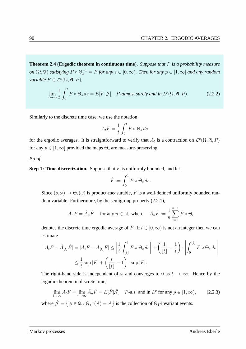
90 CHAPTER 2. ERGODIC AVERAGES
Theorem 2.4(Ergodic theorem in continuous time). Suppose thatP is a probability measure
on (Ω,A) satisfyingP Θ−1s = P for anys ∈ [0,∞). Then for anyp ∈ [1,∞] and any random
variableF ∈ Lp(Ω,A, P ),
limt→∞
1
t
ˆ t
0
F Θs ds = E[F |J ] P -almost surely and inLp(Ω,A, P ). (2.2.2)
Similarly to the discrete time case, we use the notation
AtF =1
t
ˆ t
0
F Θs ds
for the ergodic averages. It is straightforward to verify thatAt is a contraction onLp(Ω,A, P )
for anyp ∈ [1,∞] provided the mapsΘs are measure-preserving.
Proof.
Step 1: Time discretization. Suppose thatF is uniformly bounded, and let
F :=
ˆ 1
0
F Θs ds.
Since(s, ω) 7→ Θs(ω) is product-measurable,F is a well-defined uniformly bounded ran-
dom variable. Furthermore, by the semigroup property (2.2.1),
AnF = AnF for anyn ∈ N, where AnF :=1
n
n−1∑
i=0
F Θi
denotes the discrete time ergodic average ofF . If t ∈ [0,∞) is not an integer then we can
estimate
|AtF − A⌊t⌋F | = |AtF − A⌊t⌋F | ≤∣∣∣∣1
t
ˆ t
⌊t⌋F Θs ds
∣∣∣∣+(
1
⌊t⌋ − 1
t
)·∣∣∣∣∣
ˆ ⌊t⌋
0
F Θs ds
∣∣∣∣∣
≤ 1
tsup |F |+
(t
⌊t⌋ − 1
)· sup |F |.
The right-hand side is independent ofω and converges to0 as t → ∞. Hence by the
ergodic theorem in discrete time,
limt→∞
AtF = limn→∞
AnF = E[F |J ] P -a.s. and inLp for anyp ∈ [1,∞), (2.2.3)
whereJ =A ∈ A : Θ−1
1 (A) = A
is the collection ofΘ1-invariant events.
Markov processes Andreas Eberle
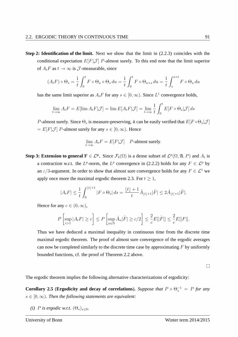
2.2. ERGODIC THEORY IN CONTINUOUS TIME 91
Step 2: Identification of the limit. Next we show that the limit in (2.2.3) coincides with the
conditional expectationE[F |J ] P -almost surely. To this end note that the limit superior
of AtF ast→ ∞ is J -measurable, since
(AtF ) Θs =1
t
ˆ t
0
F Θu Θs du =1
t
ˆ t
0
F Θu+s du =1
t
ˆ s+t
s
F Θu du
has the same limit superior asAtF for anys ∈ [0,∞). SinceL1 convergence holds,
limt→∞
AtF = E[limAtF |J ] = limE[AtF |J ] = limt→∞
1
t
ˆ t
0
E[F Θs|J ] ds
P -almost surely. SinceΘs is measure-preserving, it can be easily verified thatE[F Θs|J ]
= E[F |J ] P -almost surely for anys ∈ [0,∞). Hence
limt→∞
AtF = E[F |J ] P -almost surely.
Step 3: Extension to generalF ∈ Lp. SinceFb(Ω) is a dense subset ofLp(Ω,A, P ) andAt is
a contraction w.r.t. theLp-norm, theLp convergence in (2.2.2) holds for anyF ∈ Lp by
anε/3-argument. In order to show that almost sure convergence holds for anyF ∈ L1 we
apply once more the maximal ergodic theorem 2.3. Fort ≥ 1,
|AtF | ≤1
t
ˆ ⌊t⌋+1
0
|F Θs| ds =⌊t⌋+ 1
tA⌊t⌋+1
ˆ|F | ≤ 2A⌊t⌋+1ˆ|F |.
Hence for anyc ∈ (0,∞),
P
[supt>1
|AtF | ≥ c
]≤ P
[supn∈N
Anˆ|F | ≥ c/2
]≤ 2
cE[ ˆ|F |] ≤ 2
cE[|F |].
Thus we have deduced a maximal inequality in continuous timefrom the discrete time
maximal ergodic theorem. The proof of almost sure convergence of the ergodic averages
can now be completed similarly to the discrete time case by approximatingF by uniformly
bounded functions, cf. the proof of Theorem 2.2 above.
The ergodic theorem implies the following alternative characterizations of ergodicity:
Corollary 2.5 (Ergodicity and decay of correlations). Suppose thatP Θ−1s = P for any
s ∈ [0,∞). Then the following statements are equivalent:
(i) P is ergodic w.r.t.(Θs)s≥0.
University of Bonn Winter term 2014/2015
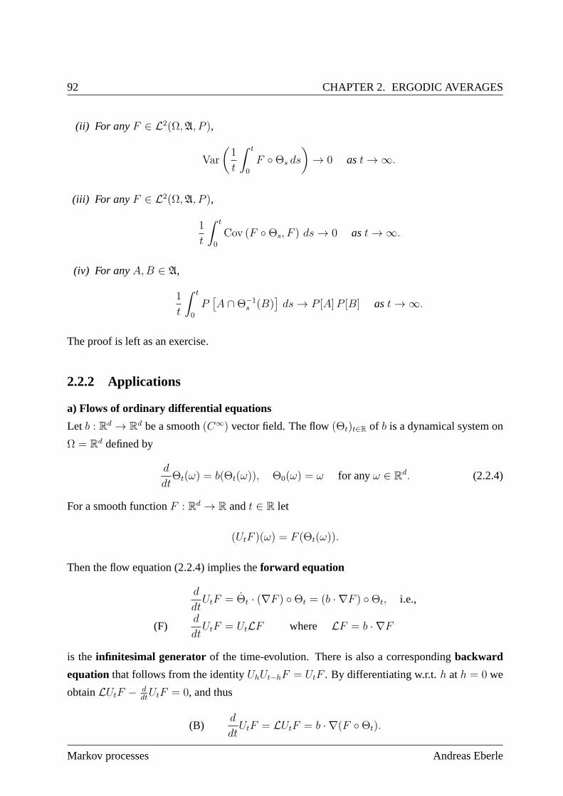
92 CHAPTER 2. ERGODIC AVERAGES
(ii) For any F ∈ L2(Ω,A, P ),
Var
(1
t
ˆ t
0
F Θs ds
)→ 0 ast→ ∞.
(iii) For any F ∈ L2(Ω,A, P ),
1
t
ˆ t
0
Cov (F Θs, F ) ds→ 0 ast→ ∞.
(iv) For anyA,B ∈ A,
1
t
ˆ t
0
P[A ∩Θ−1
s (B)]ds→ P [A]P [B] ast→ ∞.
The proof is left as an exercise.
2.2.2 Applications
a) Flows of ordinary differential equations
Let b : Rd → Rd be a smooth(C∞) vector field. The flow(Θt)t∈R of b is a dynamical system on
Ω = Rd defined by
d
dtΘt(ω) = b(Θt(ω)), Θ0(ω) = ω for anyω ∈ Rd. (2.2.4)
For a smooth functionF : Rd → R andt ∈ R let
(UtF )(ω) = F (Θt(ω)).
Then the flow equation (2.2.4) implies theforward equation
d
dtUtF = Θt · (∇F ) Θt = (b · ∇F ) Θt, i.e.,
(F)d
dtUtF = UtLF where LF = b · ∇F
is the infinitesimal generator of the time-evolution. There is also a correspondingbackward
equation that follows from the identityUhUt−hF = UtF . By differentiating w.r.t.h ath = 0 we
obtainLUtF − ddtUtF = 0, and thus
(B)d
dtUtF = LUtF = b · ∇(F Θt).
Markov processes Andreas Eberle
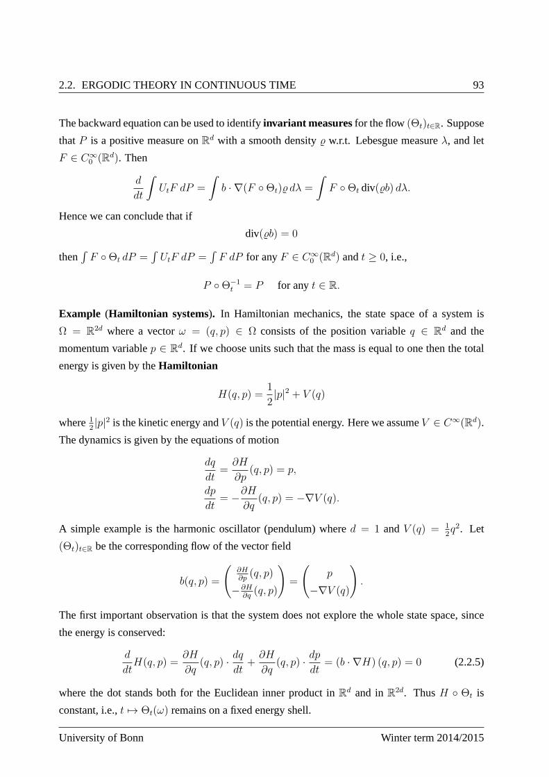
2.2. ERGODIC THEORY IN CONTINUOUS TIME 93
The backward equation can be used to identifyinvariant measuresfor the flow(Θt)t∈R. Suppose
thatP is a positive measure onRd with a smooth density w.r.t. Lebesgue measureλ, and let
F ∈ C∞0 (Rd). Then
d
dt
ˆ
UtF dP =
ˆ
b · ∇(F Θt) dλ =
ˆ
F Θt div(b) dλ.
Hence we can conclude that if
div(b) = 0
then´
F Θt dP =´
UtF dP =´
F dP for anyF ∈ C∞0 (Rd) andt ≥ 0, i.e.,
P Θ−1t = P for anyt ∈ R.
Example (Hamiltonian systems). In Hamiltonian mechanics, the state space of a system is
Ω = R2d where a vectorω = (q, p) ∈ Ω consists of the position variableq ∈ Rd and the
momentum variablep ∈ Rd. If we choose units such that the mass is equal to one then the total
energy is given by theHamiltonian
H(q, p) =1
2|p|2 + V (q)
where12|p|2 is the kinetic energy andV (q) is the potential energy. Here we assumeV ∈ C∞(Rd).
The dynamics is given by the equations of motion
dq
dt=∂H
∂p(q, p) = p,
dp
dt= −∂H
∂q(q, p) = −∇V (q).
A simple example is the harmonic oscillator (pendulum) where d = 1 andV (q) = 12q2. Let
(Θt)t∈R be the corresponding flow of the vector field
b(q, p) =
(∂H∂p
(q, p)
−∂H∂q(q, p)
)=
(p
−∇V (q)
).
The first important observation is that the system does not explore the whole state space, since
the energy is conserved:
d
dtH(q, p) =
∂H
∂q(q, p) · dq
dt+∂H
∂q(q, p) · dp
dt= (b · ∇H) (q, p) = 0 (2.2.5)
where the dot stands both for the Euclidean inner product inRd and inR2d. ThusH Θt is
constant, i.e.,t 7→ Θt(ω) remains on a fixed energy shell.
University of Bonn Winter term 2014/2015
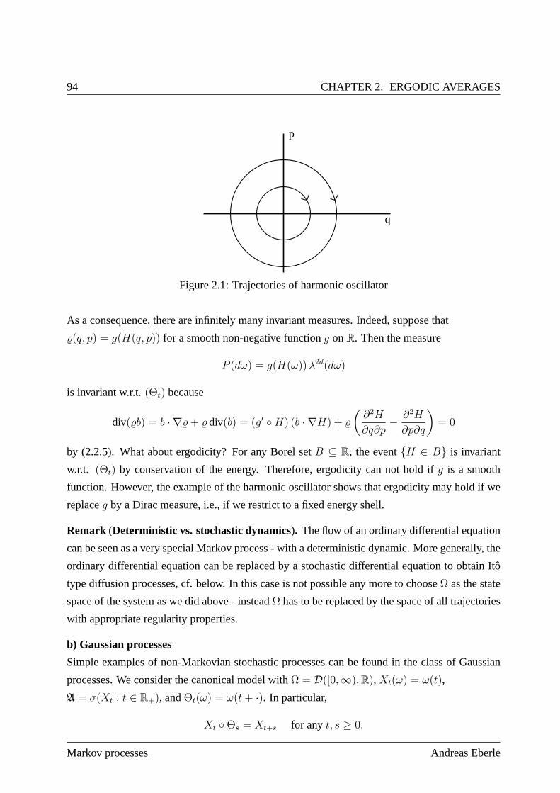
94 CHAPTER 2. ERGODIC AVERAGES
p
q
Figure 2.1: Trajectories of harmonic oscillator
As a consequence, there are infinitely many invariant measures. Indeed, suppose that
(q, p) = g(H(q, p)) for a smooth non-negative functiong onR. Then the measure
P (dω) = g(H(ω))λ2d(dω)
is invariant w.r.t.(Θt) because
div(b) = b · ∇+ div(b) = (g′ H) (b · ∇H) +
(∂2H
∂q∂p− ∂2H
∂p∂q
)= 0
by (2.2.5). What about ergodicity? For any Borel setB ⊆ R, the eventH ∈ B is invariant
w.r.t. (Θt) by conservation of the energy. Therefore, ergodicity can not hold if g is a smooth
function. However, the example of the harmonic oscillator shows that ergodicity may hold if we
replaceg by a Dirac measure, i.e., if we restrict to a fixed energy shell.
Remark (Deterministic vs. stochastic dynamics). The flow of an ordinary differential equation
can be seen as a very special Markov process - with a deterministic dynamic. More generally, the
ordinary differential equation can be replaced by a stochastic differential equation to obtain Itô
type diffusion processes, cf. below. In this case is not possible any more to chooseΩ as the state
space of the system as we did above - insteadΩ has to be replaced by the space of all trajectories
with appropriate regularity properties.
b) Gaussian processes
Simple examples of non-Markovian stochastic processes canbe found in the class of Gaussian
processes. We consider the canonical model withΩ = D([0,∞),R),Xt(ω) = ω(t),
A = σ(Xt : t ∈ R+), andΘt(ω) = ω(t+ ·). In particular,
Xt Θs = Xt+s for anyt, s ≥ 0.
Markov processes Andreas Eberle
2.2. ERGODIC THEORY IN CONTINUOUS TIME 95
Let P be a probability measure on(Ω,A). The stochastic process(Xt, P ) is called aGaussian
processif and only if (Xt1 , . . . , Xtn) has a multivariate normal distribution for anyn ∈ N and
t1, . . . , tn ∈ R+ (Recall that it is not enough to assume thatXt is normally distributed for anyt!).
The lawP of a Gaussian process is uniquely determined by the averagesand covariances
m(t) = E[Xt], c(s, t) = Cov(Xs, Xt), s, t ≥ 0.
It can be shown (Exercise) that a Gaussian process is stationary if and only ifm(t) is constant,
and
c(s, t) = r(|s− t|)
for some functionr : R+ → R (auto-correlation function). To obtain a necessary condition for
ergodicity note that if(Xt, P ) is stationary and ergodic then1t
´ t
0Xs ds converges to the constant
averagem, and hence
Var
(1
t
ˆ t
0
Xs ds
)→ 0 ast→ ∞.
On the other hand, by Fubini’s theorem,
Var
(1
t
ˆ t
0
Xs ds
)= Cov
(1
t
ˆ t
0
Xs ds,1
t
ˆ t
0
Xu du
)
=1
t2
ˆ t
0
ˆ t
0
Cov (Xs, Xu) duds =1
2t2
ˆ t
0
ˆ s
0
r(s− u) duds
=1
2t2
ˆ t
0
(t− v)r(v) dv =1
2t
ˆ t
0
(1− v
t
)r(v) dv
∼ 1
2t
ˆ t
0
r(v)dv asymptotically ast→ ∞.
Hence ergodicity can only hold if
limt→∞
1
t
ˆ t
0
r(v) dv = 0.
It can be shown by Spectral analysis/Fourier transform techniques that this condition is also suf-
ficient for ergodicity, cf e.g. Lindgren, “Lectures on Stationary Stochastic Processes” [20].
c) Random Fields
We have stated the ergodic theorem for temporal, i.e., one-dimensional averages. There are
corresponding results in the multi-dimensional case, i.e., t ∈ Zd or t ∈ Rd, cf. e.g. Strook,
“Probability Theory: An Analytic View”. [34]. These apply for instance to ergodic averages of
the form
AtF =1
(2t)d
ˆ
(−t,t)dF Θs ds, t ∈ R+,
University of Bonn Winter term 2014/2015
96 CHAPTER 2. ERGODIC AVERAGES
where(Θs)s∈Rd is a group of measure-preserving transformations on a probability space(Ω,A, P ).
Multi-dimensional ergodic theorems are important to the study of stationary random fields. Here
we just mention briefly two typical examples:
Example (Massless Gaussian free field onZd). LetΩ = RZdwhered ≥ 3, and letXs(ω) = ωs
for ω = (ωs) ∈ Ω. Themassless Gaussian free fieldis the probability measureP onΩ given
informally by
“P (dω) =1
Zexp
(− 1
2
∑
s,t∈Zd
|s−t|=1
|ωt − ωs|2)∏
s∈Zd
dωs ” . (2.2.6)
The expression is not rigorous since the Gaussian free field on RZddoes not have a density
w.r.t. a product measure. Indeed, the density in (2.2.6) would be infinite for almost everyω.
Nevertheless,P can be defined rigorously as the law of a centered Gaussian process (or random
field) (Xs)s∈Zd with covariances
Cov(Xs, Xt) = G(s, t) for anys, t ∈ Zd,
whereG(s, t) =∞∑n=0
pn(s, t) is the Green’s function of the Random Walk onZd. The connection
to the informal expression in (2.2.6) is made by observing that the generator of the random walk
is the discrete Laplacian∆Zd , and the informal density in (2.2.6) takes the form
Z−1 exp
(−1
2(ω,∆Zdω)l2(Zd)
).
For d ≥ 3, the random walk onZd is transient. Hence the Green’s function is finite, and one
can show that there is a unique centered Gaussian measureP on Ω with covariance function
G(s, t). Since G(s, t) depends only ons − t, the measureP is stationary w.r.t. the shift
Θs(ω) = ω(s+ ·), s ∈ Zd. Furthermore, decay of correlation holds ford ≥ 3 since
G(s, t) ∼ |s− t|2−d as|s− t| → ∞.
It can be shown that this implies ergodicity ofP , i.e., theP -almost sure limits of spatial ergodic
averages are constant. In dimensionsd = 1, 2 the Green’s function is infinite and the massless
Gaussian free field does not exist. However, in any dimensiond ∈ N it is possible to define
in a similar way the Gaussian free field with massm ≥ 0, whereG is replaced by the Green’s
function of the operatorm2 −∆Zd.
Example (Markov chains in random environment). Suppose that(Θx)x∈Zd is stationary and
ergodic on a probability space(Ω,A, P ), and letq : Ω× Zd → [0, 1] be a stochastic kernel from
Ω to Zd. Then random transition probabilities onZd can be defined by setting
p(ω, x, y) = q (Θx(ω), y − x) for anyω ∈ Ω andx, y ∈ Zd.
Markov processes Andreas Eberle
2.2. ERGODIC THEORY IN CONTINUOUS TIME 97
For any fixedω ∈ Ω, p(ω, ·) is the transition matrix of a Markov chain onZd. The variableω
is called therandom environment - it determines which transition matrix is applied. One is
now considering a two-stage model where at first an environment ω is chosen at random, and
then (givenω) a Markov chain is run in this environment. Typical questions that arise are the
following:
• Quenched asymptotics.How does the Markov chain with transition kernelp(ω, ·, ·) be-
have asymptotically for a typicalω (i.e., forP -almost everyω ∈ Ω)?
• Annealed asymptotics.What can be said about the asymptotics if one is averaging overω
w.r.t. P?
For an introduction to these and other questions see e.g. Sznitman, “Ten lectures on Random
media” [3].
2.2.3 Ergodic theory for Markov processes
We now return to our main interest in these notes: The application of ergodic theorems to
Markov processes in continuous time. Suppose that(pt)t∈[0,∞) is a transition function of a time-
homogeneous Markov process(Xt, Pµ) on (Ω,A). We assume that(Xt)t∈[0,∞) is the canonical
process onΩ = D([0,∞), S), A = σ(Xt : t ∈ [0,∞)), andµ is the law ofX0 w.r.t. Pµ. The
measureµ is a stationary distribution for(pt) iff
µpt = µ for anyt ∈ [0,∞).
The existence of stationary distributions can be shown similarly to the discrete time case:
Theorem 2.6(Krylov-Bogolinbov ). Suppose that the family
νpt =1
t
ˆ t
0
νps ds, t ≥ 0,
of probability measures onS is tight for someν ∈ P(S). Then there exists a stationary distribu-
tion µ of (pt)t≥0.
The proof of this and of the next theorem are left as exercises.
University of Bonn Winter term 2014/2015
98 CHAPTER 2. ERGODIC AVERAGES
Theorem 2.7(Characterizations of ergodicity in continuous time). 1) The shift semi-
groupΘs(ω) = ω(t + ·), t ≥ 0, preserves the measurePµ if and only ifµ is a stationary
distribution for(pt)t≥0.
2) In this case, the following statements are all equivalent
(i) Pµ is ergodic.
(ii) For any f ∈ L2(S, µ),
1
t
ˆ t
0
f(Xs) ds→ˆ
f dµ Pµ-a.s. ast→ ∞.
(iii) For any f ∈ L2(S, µ),
VarPµ
(1
t
ˆ t
0
f(Xs) ds
)→ 0 ast→ ∞.
(iv) For anyf, g ∈ L2(S, µ),
1
t
ˆ t
0
CovPµ (g(X0), f(Xs)) ds→ 0 ast→ ∞.
(v) For anyA,B ∈ B,
1
t
ˆ t
0
Pµ [X0 ∈ A,Xs ∈ B] ds→ µ(A)µ(B) ast→ ∞.
(vi) For anyB ∈ B,
1
t
ˆ t
0
ps(x,B) ds→ µ(B) µ-a.e. ast→ ∞.
(vii) For anyB ∈ B with µ(B) > 0,
Px[TB <∞] > 0 for µ-a.e.x ∈ S.
(viii) For anyB ∈ B such thatpt1B = 1B µ-a.e. for anyt ≥ 0,
µ(B) ∈ 0, 1.
(ix) Any functionh ∈ Fb(S) satisfyingpth = h µ-a.e. for anyt ≥ 0 is constant up to a
set ofµ-measure zero.
Markov processes Andreas Eberle
2.2. ERGODIC THEORY IN CONTINUOUS TIME 99
One way to verify ergodicity is the strong Feller property:
Definition (Strong Feller property). A transition kernelp on (S,B) is calledstrong Feller iff
pf is continuous for any bounded measurable functionf : S → R.
Corollary 2.8. Suppose that one of the transition kernelspt, t > 0, is strong Feller. ThenPµ is
stationary and ergodic for any stationary distributionµ of (pt)t≥0 that as connected support.
Proof. LetB ∈ B such that
pt1B = 1B µ-a.e. for anyt ≥ 0. (2.2.7)
By Theorem 2.7 it suffices to showµ(B) ∈ 0, 1. If pt is strong Feller for somet thenpt1B
is a continuous function. Therefore, by (2.2.7) and since the support ofµ is connected, either
pt1B ≡ 0 or pt1B ≡ 1 on supp(µ). Hence
µ(B) = µ(1B) = µ(pt1B) ∈ 0, 1.
Example (Brownian motion on R/Z). A Brownian motion(Xt) on the circleR/Z can be
obtained by considering a Brownian motion(Bt) onR modulo the integers, i.e.,
Xt = Bt − ⌊Bt⌋ ∈ [0, 1) ⊆ R/Z.
Since Brownian motion onR has the smooth transition density
pRt (x, y) = (2πt)−1/2 exp(−|x− y|2/(2t)),
the transition density of Brownian motion onR/Z w.r.t. the uniform distribution is given by
pt(x, y) =∑
n∈Zpt(x, y + n) =
1√2πt
e−|x−y−n|2
2t for anyt > 0 andx, y ∈ [0, 1).
Sincept is a smooth function with bounded derivatives of all orders,the transition kernels are
strong Feller for anyt > 0. The uniform distribution onR/Z is stationary for(pt)t≥0. Therefore,
by Corollary 2.8, Brownian motion onR/Z with uniform initial distribution is a stationary and
ergodic Markov process.
A similar reasoning as in the last example can be carried out for general non-degenerate diffusion
processes onRd. These are Markov processes generated by a second order differential operator
of the form
L =1
2
d∑
i,j=1
aij(x)∂2
∂xi∂xj+
d∑
i=1
bi(x)∂
∂xi.
University of Bonn Winter term 2014/2015
100 CHAPTER 2. ERGODIC AVERAGES
By PDE theory it can be shown that if the coefficients are locally Hölder continuous, the matrix
(aij(x)) is non-degenerate for anyx, and appropriate growth conditions hold at infinity then there
is a unique transition semigroup(pt)t≥0 with a smooth transition density corresponding toL, cf.
e.g. [XXX]. Therefore, Corollary 2.8 can be applied to prove that the law of a corresponding
Markov process with stationary initial distribution is stationary and ergodic.
2.3 Structure of invariant measures
In this section we apply the ergodic theorem to study the structure of the set of all invariant
measures w.r.t. a given one-parameter family of transformations(Θt)t≥0 as well as the structure
of the set of all stationary distributions of a given transition semigroup(pt)t≥0.
2.3.1 The convex set ofΘ-invariant probability measures
LetΘ : R+×Ω → Ω, (t, ω) 7→ Θt(ω) be product-measurable on(Ω,A) satisfying the semigroup
property
Θ0 = idΩ, Θt Θs = Θt+s for anyt, s ≥ 0,
and letJ =A ∈ A : Θ−1
t (A) = A for anyt ≥ 0
. Alternatively, the results will also hold in
the discrete time case, i.e.,R+ may be replaced byZ+. We denote by
S(Θ) =P ∈ P(Ω) : P Θ−1
t = P for anyt ≥ 0
the set of all(Θt)-invariant (stationary) probability measures on(Ω,A).
Lemma 2.9(Singularity of ergodic probability measures). SupposeP,Q ∈ S(Θ) are distinct
ergodic probability measures. ThenP andQ are singular on theσ-algebraJ , i.e., there exist an
eventA ∈ J such thatP [A] = 1 andQ[A] = 0.
Proof. This is a direct consequence of the ergodic theorem. IfP 6= Q then there is a random
variableF ∈ Fb(Ω) such that´
F dP 6=´
F dQ. The event
A :=
lim supt→∞
AtF =
ˆ
F dP
is contained inJ , and by the ergodic theorem,P [A] = 1 andQ[A] = 0.
Recall that an elementx in a convex setC is called an extreme point ofC if x can not be
represented in a non-trivial way as a convex combination of elements inC. The setCe of all
extreme points inC is hence given by
Ce = x ∈ C : x1, x2 ∈ C\x, α ∈ (0, 1) : x = αx1 + (1− α)x2 .
Markov processes Andreas Eberle
2.3. STRUCTURE OF INVARIANT MEASURES 101
Theorem 2.10(Structure and extremals ofS(Θ)). 1) The setS(Θ) is convex.
2) A (Θt)-invariant probability measureP is extremal inS(Θ) if and only ifP is ergodic.
3) If Ω is a polish space andA is the Borelσ-algebra then any(Θt)-invariant probability
measureP on (Ω,A) can be represented as a convex combination of extremal (ergodic)
elements inS(Θ), i.e., there exists a probability measure onS(Θ)e such that
P =
ˆ
S(Θ)e
Q(dQ).
Proof. 1) If P1 andP2 are(Θt)-invariant probability measures then any convex combination
αP1 + (1− α)P2, α ∈ [0, 1], is (Θt)-invariant, too.
2) Suppose first thatP ∈ S(Θ) is ergodic andP = αP1 + (1− α)P2 for someα ∈ (0, 1) and
P1, P2 ∈ S(Θ). ThenP1 andP2 are both absolutely continuous w.r.t.P . HenceP1 and
P2 are ergodic, i.e., they only take the values0 and1 on sets inJ . Since distinct ergodic
measures are singular by Lemma 2.9 we can conclude thatP1 = P = P2, i.e., the convex
combination is trivial. This showsP ∈ S(Θ)e.
Conversely, suppose thatP ∈ S(Θ) is not ergodic, and letA ∈ J such thatP [A] ∈ (0, 1).
ThenP can be represented as a non-trivial combination by conditioning onσ(A):
P = P [ · |A]P [A] + P [ · |Ac]P [Ac].
As A is in J , the conditional distributionsP [ · |A] andP [ · |Ac] are both(Θt)-invariant
again. HenceP /∈ S(Θ)e.
3) This part is a bit tricky, and we only sketch the main idea. For more details see e.g. Varad-
han, “Probability Theory” [36]. Since(Ω,A) is a polish space with Borelσ-algebra, there
is a regular versionpJ (ω, ·) of the conditional distributionsP [ · |J ](ω) given theσ-algebra
J . Furthermore, it can be shown thatpJ (ω, ·) is stationary andergodic for P -almost
everyω ∈ Ω (The idea in the background is that we “divide out” the non-trivial invariant
University of Bonn Winter term 2014/2015
102 CHAPTER 2. ERGODIC AVERAGES
events by conditioning onJ ). Assuming the ergodicity ofpJ (ω, ·) for P -a.e.ω, we obtain
the representation
P (dω) =
ˆ
pJ (ω, ·)P (dω)
=
ˆ
S(Θ)e
Q(dQ)
where is the law ofω 7→ pJ (ω, ·) underP . Here we have used the definition of a
regular version of the conditional distribution and the transformation theorem for Lebesgue
integrals.
To prove ergodicity ofpJ (ω, ·) for almost everyω one can use that a measure is ergodic if
and only if all limits of ergodic averages of indicator functions are almost surely constant.
For a fixed eventA ∈ A,
limt→∞
1
t
ˆ t
0
1A Θs ds = P [A|J ] P -almost surely, and thus
limt→∞
1
t
ˆ t
0
1A Θs ds = pJ (ω,A) pJ (ω, ·)-almost surely forP -a.e.ω.
The problem is that the exceptional set in “P -almost every” depends onA, and there are
uncountably many eventsA ∈ A in general. To resolve this issue, one can use that the Borel
σ-algebra on a Polish space is generated by countably many sets An. The convergence
above then holds simultaneously with the same exceptional set for allAn. This is enough
to prove ergodicity ofpJ (ω, ·) for P -almost everyω.
2.3.2 The set of stationary distributions of a transition semigroup
We now specialize again to Markov processes. Letp = (pt)t≥0 be a transition semigroup on
(S,B), and let(Xt, Px) be a corresponding canonical Markov process onΩ = D(R+, S). We
now denote byS(p) the collection of all stationary distributions for(pt)t≥0, i.e.,
S(p) = µ ∈ P(S) : µ = µpt for anyt ≥ 0 .
As usually in this setup,J is theσ-algebra of events inA = σ(Xt : t ≥ 0) that are invariant
under time-shiftsΘt(ω) = ω(t+ ·).
Exercise(Shift-invariants events for Markov processes). Show that for anyA ∈ J there exists
a Borel setB ∈ B such thatpt1B = 1B µ-almost surely for anyt ≥ 0, and
A =⋂
n∈N
⋃
m≥n
Xm ∈ B = X0 ∈ B P -almost surely.
Markov processes Andreas Eberle
2.4. QUANTITATIVE BOUNDS & CLT FOR ERGODIC AVERAGES 103
The next result is an analogue to Theorem 2.10 for Markov processes. It can be either deduced
from Theorem 2.10 or proven independently.
Theorem 2.11(Structure and extremals ofS(p)). 1) The setS(p) is convex.
2) A stationary distributionµ of (pt) is extremal inS(p) if and only if any setB ∈ B such that
pt1B = 1B µ-a.s. for anyt ≥ 0 has measureµ(B) ∈ 0, 1.
3) Any stationary distributionµ of (pt) can be represented as a convex combination of ex-
tremal elements inS(p).
Remark (Phase transitions). The existence of several stationary distributions can correspond
to the occurrence of a phase transition. For instance we willsee in XXX below that for the heat
bath dynamics of the Ising model onZd there is only one stationary distribution above the critical
temperature but there are several stationary distributions in the phase transition regime below the
critical temperature.
2.4 Quantitative bounds & CLT for ergodic averages
Let (pt)t≥0 be the transition semigroup of a Markov process((Xt)t∈Z+ , Px) in discrete time or a
right-continuous Markov process((Xt)t∈R+ , Px) in continuous time with state space(S,B). In
discrete time,pt = pt wherep is the one-step transition kernel. Suppose thatµ is a stationary
distribution of(pt)t≥0. If ergodicity holds then by the ergodic theorem, the averages
Atf =1
t
t−1∑
i=0
f(Xi), Atf =1
t
ˆ t
0
f(Xs) ds respectively,
converge toµ(f) =´
fdµ for anyf ∈ L1(µ). In this section, we study the asymptotics of the
functions ofAtf aroundµ(f) ast→ ∞ for f ∈ L2(µ).
2.4.1 Bias and variance of stationary ergodic averages
Theorem 2.12(Bias, variance and asymptotic variance of ergodic averages). Let f ∈ L2(µ)
and letf0 = f − µ(f). The following statements hold:
University of Bonn Winter term 2014/2015
104 CHAPTER 2. ERGODIC AVERAGES
1) For anyt > 0, Atf is an unbiased estimator forµ(f) w.r.t. Pµ, i.e.,
EPµ [Atf ] = µ(f).
2) The variance ofAtf in stationarity is given by
VarPµ [Atf ] =1
tVarµ(f) +
2
t
t∑
k=1
(1− k
t
)Covµ(f, p
kf) in discrete time,
VarPµ [Atf ] =2
t
ˆ t
0
(1− r
t
)Covµ(f, prf)dr in continuous time, respectively.
3) Suppose that the seriesGf0 =∞∑k=0
pkf0 or the integralGf0 =´∞0psf0 ds (in discrete/
continuous time respectively) converges inL2(µ). Then the asymptotic variance of√tAtf
is given by
limt→∞
t · VarPµ [Atf ] = σ2f , where
σ2f = Varµ(f) + 2
∞∑
k=1
Covµ(f, pkf) = 2(f0, Gf0)L2(µ) − (f0, f0)L2(µ)
in the discrete time case, and
σ2f =
ˆ ∞
0
Covµ(f, psf)ds = 2(f0, Gf0)L2(µ)
in the continuous time case, respectively.
Remark. 1) The asymptotic variance equals
σ2f = VarPµ [f(X0)] + 2
∞∑
k=1
CovPµ [f(X0), f(Xk)],
σ2f =
ˆ ∞
0
CovPµ [f(X0), f(Xs)]ds respectively.
If Gf0 exists then the variance of the ergodic averages behaves asymptotically asσ2f/t.
2) The statement hold under the assumption that the Markov process is started in stationarity.
Bounds for ergodic averages of Markov processes with non-stationary initial distribution
are given in Section 2.5 below.
Proof of Theorem 2.12:
We prove the results in the continuous time case. The analogue discrete time case is left as
Markov processes Andreas Eberle
2.4. QUANTITATIVE BOUNDS & CLT FOR ERGODIC AVERAGES 105
an exercise. Note first that by right-continuity of(Xt)t≥0, the process(s, ω) 7→ f(Xs(ω)) is
product-measurable and square integrable on[0, t]× Ω w.r.t. λ⊗ Pµ for anyt ∈ R+.
1) By Fubini’s theorem and stationarity,
EPµ
[1
t
ˆ t
0
f(Xs) ds
]=
1
t
ˆ t
0
EPµ [f(Xs)] ds = µ(f) for anyt > 0.
2) Similarly, by Fubini’s theorem, stationarity and the Markov property,
VarPµ [Atf ] = CovPµ
[1
t
ˆ t
0
f(Xs) ds,1
t
ˆ t
0
f(Xu) du
]
=2
t2
ˆ t
0
ˆ u
0
CovPµ [f(Xs), f(Xu)] dsdu
=2
t2
ˆ t
0
ˆ u
0
Covµ(f, pu−sf) dsdu
=2
t2
ˆ t
0
(t− r) Covµ(f, prf) dr.
3) Note that by stationarity,µ(prf) = µ(f), and hence
Covµ(f, prf) =
ˆ
f0 prf0 dµ for anyr ≥ 0.
Therefore, by 2) and Fubini’s theorem,
t · VarPµ [Atf ] = 2
ˆ t
0
(1− r
t
)ˆf0 prf0 dµdr
= 2
(f0,
ˆ t
0
(1− r
t
)prf0 dr
)
L2(µ)
→ 2
(f0,
ˆ ∞
0
prf0 dr
)
L2(µ)
ast→ ∞
provided the integral´∞0prf0 dr converges inL2(µ). Here the last conclusion holds since
L2(µ)-convergence of´ t
0prf0 dr ast→ ∞ implies that
ˆ t
0
r
tprf0 dr =
1
t
ˆ t
0
ˆ r
0
prf0 dsdr =1
t
ˆ t
0
ˆ t
s
prf0 drds→ 0 in L2(µ) ast→ ∞.
Remark (Potential operator, existence of asymptotic variance). The theorem states that the
asymptotic variance of√tAtf exists if the series/integralGf0 converges inL2(µ). Notice thatG
is a linear operator that is defined in the same way as the Green’s function. However, the Markov
University of Bonn Winter term 2014/2015
106 CHAPTER 2. ERGODIC AVERAGES
process is recurrent due to stationarity, and thereforeG1B = ∞ µ-a.s. onB for any Borel setB ⊆S. Nevertheless,Gf0 often exists becausef0 has meanµ(f0) = 0. Some sufficient conditions
for the existence ofGf0 (and hence of the asymptotic variance) are given in the exercise below.
If Gf0 exists for anyf ∈ L2(µ) thenG induces a linear operator on the Hilbert space
L20(µ) = f ∈ L2(µ) : µ(f) = 0,
i.e., on the orthogonal complement of the constant functions in L2(µ). This linear operator is
called thepotential operator. It is the inverse of the negative generator restricted to the orthog-
onal complement of the constant functions. Indeed, in discrete time,
−LGf0 = (I − p)∞∑
n=0
pnf0 = f0
wheneverGf0 converges. Similarly, in continuous time, ifGf0 exists then
−LGf0 = − limh↓0
ph − I
h
ˆ ∞
0
ptf0 dt = limh↓0
1
h
(ˆ ∞
0
ptf0 dt−ˆ ∞
0
pt+hf0 dt
)
= limh↓0
1
h
ˆ h
0
ptf0 dt = f0.
The last conclusion holds by strong continuity oft 7→ ptf0, cf. Theorem 3.11 below.
Exercise (Sufficient conditions for existence of the asymptotic variance). Prove that in the
continuous time case,Gf0 =´∞0ptf0 converges inL2(µ) if one of the following conditions is
satisfied:
(i) Decay of correlations:´∞0
∣∣CovPµ [f(X0), f(Xt)]∣∣ dt <∞.
(ii) L2 bound:´∞0
‖ptf0‖L2(µ)dt <∞.
Deduce non-asymptotic (t finite) and asymptotic (t → ∞) bounds for the variances of ergodic
averages under the assumption that either the correlations|CovPµ [f(X0), f(Xt)]| or theL2(µ)
norms‖ptf0‖L2(µ) are bounded by an integrable functionr(t).
2.4.2 Central limit theorem for Markov chains
We now restrict ourselves to the discrete time case. Letf ∈ L2(µ), and suppose that the asymp-
totic variance
σ2f = lim
n→∞nVarPµ [Anf ]
Markov processes Andreas Eberle
2.4. QUANTITATIVE BOUNDS & CLT FOR ERGODIC AVERAGES 107
exists and is finite. Without loss of generality we assumeµ(f) = 0, otherwise we may consider
f0 instead off . Our goal is to prove a central limit theorem of the form
1√n
n−1∑
i=0
f(Xi)D→ N(0, σ2
f ) (2.4.1)
where “D→” stands for convergence in distribution. The key idea is to use the martingale problem
in order to reduce (2.4.1) to a central limit theorem for martingales. Ifg is a function inL2(µ)
theng(Xn) ∈ L2(Pµ) for anyn ≥ 0, and hence
g(Xn)− g(X0) =Mn +n−1∑
k=0
(Lg)(Xk) (2.4.2)
where(Mn) is a square-integrable(FXn ) martingale withM0 = 0 w.r.t. Pµ, andLg = pg − g.
Now suppose that there exists a functiong ∈ L2(µ) such thatLg = −f µ-a.e. Note that this is
always the case withg = Gf if Gf =∞∑n=0
pnf converges inL2(µ). Then by (2.4.2),
1√n
n−1∑
k=0
f(Xk) =Mn√n+g(X0)− g(Xn)√
n. (2.4.3)
As n → ∞, the second summand converges to0 in L2(Pµ). Therefore, (2.4.1) is equivalent to a
central limit theorem for the martingale(Mn). Explicitly,
Mn =n∑
i=1
Yi for anyn ≥ 0,
where the martingale incrementsYi are given by
Yi =Mi −Mi−1 = g(Xi)− g(Xi−1)− (Lg)(Xi−1)
= g(Xi)− (pg)(Xi−1).
These increments form a stationary sequence w.r.t.Pµ. Thus we can apply the following theorem:
Theorem 2.13(CLT for martingales with stationary increments ). Let (Fn) be a filtration on
a probability space(Ω,A, P ). Suppose thatMn =n∑
i=1
Yi is an(Fn) martingale on(Ω,A, P ) with
stationary incrementsYi ∈ L2(P ), and letσ ∈ R+. If
1
n
n∑
i=1
Y 2i → σ2 in L1(P ) asn→ ∞ (2.4.4)
then1√nMn
D→ N(0, σ2) w.r.t. P. (2.4.5)
University of Bonn Winter term 2014/2015
108 CHAPTER 2. ERGODIC AVERAGES
The proof of Theorem 2.13 will be given at the end of this section. Note that by the ergodic
theorem, the condition (2.4.4) is satisfied withσ2 = E[Y 2i ] if the process(Yi, P ) is ergodic. As
consequence of Theorem 2.13 and the considerations above, we obtain:
Corollary 2.14 (CLT for stationary Markov chains ). Let (Xn, Pµ) be a stationary and ergodic
Markov chain with initial distributionµ and one-step transition kernelp, and letf ∈ L2(µ).
Suppose that there exists a functiong ∈ L2(µ) such that
− Lg = f − µ(f). (2.4.6)
Then asn→ ∞,
1√n
n−1∑
k=0
(f(Xk)− µ(f))D→ N(0, σ2
f ), where
σ2f = 2Covµ(f, g)− Varµ(f).
Remark. Recall that (2.4.6) is satisfied withg = G(f − µ(f)) if it exists.
Proof. Let Yi = g(Xi) − (pg)(Xi−1). Then underPµ (Yi) is a stationary sequence of square-
integrable martingale increments. By the ergodic theorem, for the process(Xn, Pµ),
1
n
n∑
i=1
Y 2i → Eµ[Y
21 ] in L1(Pµ) asn→ ∞.
The limiting expectation can be identified as the asymptoticvarianceσ2f by an explicit computa-
tion:
Eµ[Y21 ] = Eµ[(g(X1)− (pg)(X0))
2]
=
ˆ
µ(dx)Ex[g(X1)2 − 2g(X1)(pg)(X0) + (pg)(X0)
2]
=
ˆ
(pg2 − 2(pg)2 + (pg)2)dµ =
ˆ
g2 dµ−ˆ
(pg)2dµ
= (g − pg, g + pg)L2(µ) = 2(f0, g)L2(µ) − (f0, f0)L2(µ) = σ2f .
Heref0 := f − µ(f) = −Lg = g − pg by assumption. The martingale CLT 2.13 now implies
that1√n
n∑
i=1
YiD→ N(0, σ2
f ),
and hence
1√n
n−1∑
i=0
(f(Xi)− µ(f)) =1√n
n∑
i=1
Yi +g(X0)− g(Xn)√
n
D→ N(0, σ2f )
as well, becauseg(X0)− g(Xn) is bounded inL2(Pµ).
Markov processes Andreas Eberle
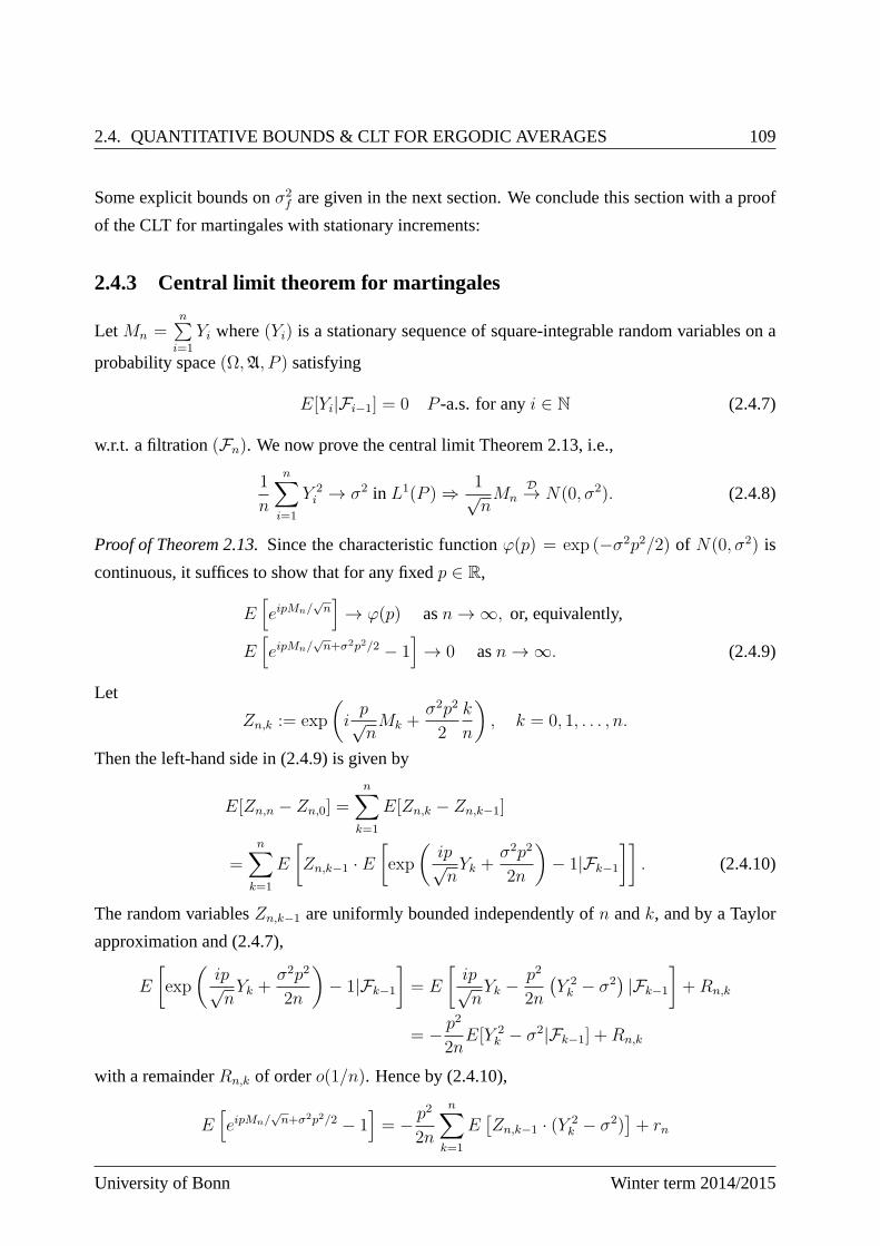
2.4. QUANTITATIVE BOUNDS & CLT FOR ERGODIC AVERAGES 109
Some explicit bounds onσ2f are given in the next section. We conclude this section with aproof
of the CLT for martingales with stationary increments:
2.4.3 Central limit theorem for martingales
LetMn =n∑
i=1
Yi where(Yi) is a stationary sequence of square-integrable random variables on a
probability space(Ω,A, P ) satisfying
E[Yi|Fi−1] = 0 P -a.s. for anyi ∈ N (2.4.7)
w.r.t. a filtration(Fn). We now prove the central limit Theorem 2.13, i.e.,
1
n
n∑
i=1
Y 2i → σ2 in L1(P ) ⇒ 1√
nMn
D→ N(0, σ2). (2.4.8)
Proof of Theorem 2.13.Since the characteristic functionϕ(p) = exp (−σ2p2/2) of N(0, σ2) is
continuous, it suffices to show that for any fixedp ∈ R,
E[eipMn/
√n]→ ϕ(p) asn→ ∞, or, equivalently,
E[eipMn/
√n+σ2p2/2 − 1
]→ 0 asn→ ∞. (2.4.9)
Let
Zn,k := exp
(ip√nMk +
σ2p2
2
k
n
), k = 0, 1, . . . , n.
Then the left-hand side in (2.4.9) is given by
E[Zn,n − Zn,0] =n∑
k=1
E[Zn,k − Zn,k−1]
=n∑
k=1
E
[Zn,k−1 · E
[exp
(ip√nYk +
σ2p2
2n
)− 1|Fk−1
]]. (2.4.10)
The random variablesZn,k−1 are uniformly bounded independently ofn andk, and by a Taylor
approximation and (2.4.7),
E
[exp
(ip√nYk +
σ2p2
2n
)− 1|Fk−1
]= E
[ip√nYk −
p2
2n
(Y 2k − σ2
)|Fk−1
]+Rn,k
= − p2
2nE[Y 2
k − σ2|Fk−1] +Rn,k
with a remainderRn,k of ordero(1/n). Hence by (2.4.10),
E[eipMn/
√n+σ2p2/2 − 1
]= − p2
2n
n∑
k=1
E[Zn,k−1 · (Y 2
k − σ2)]+ rn
University of Bonn Winter term 2014/2015
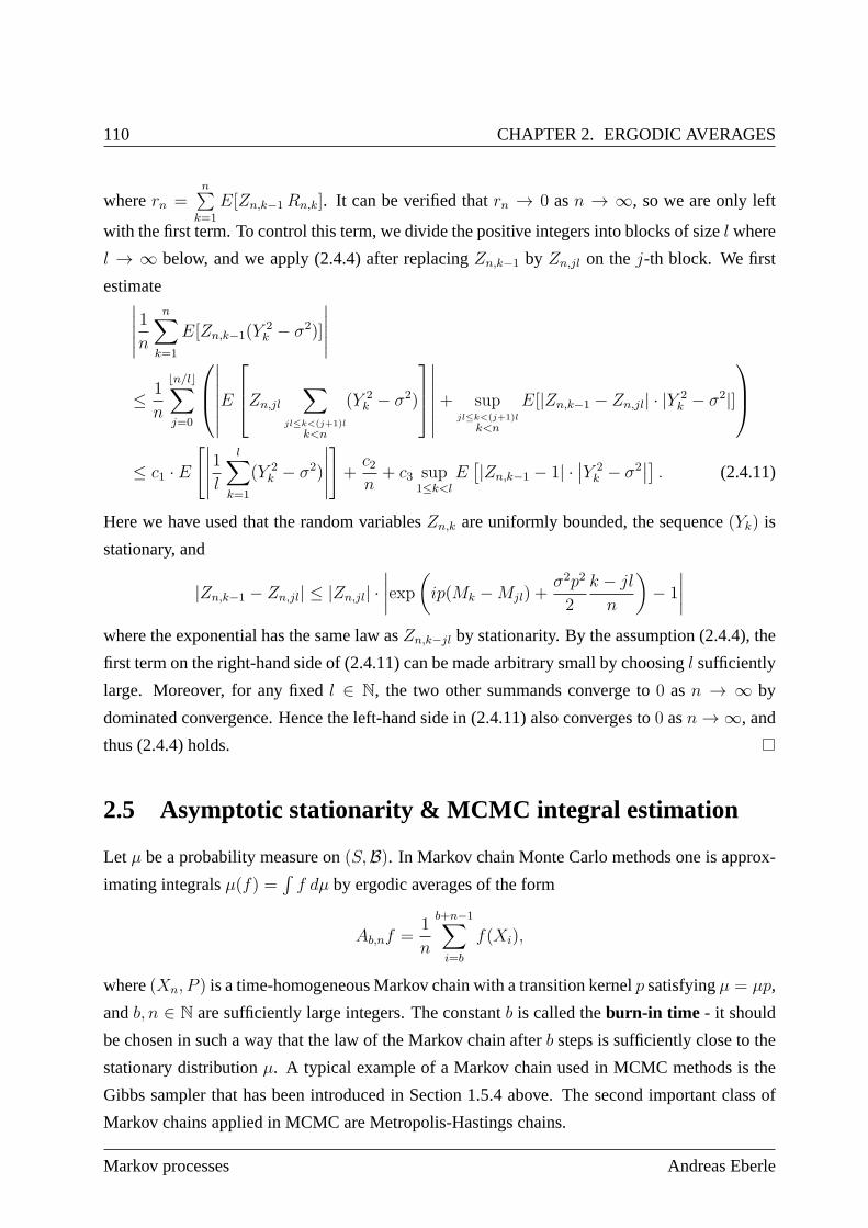
110 CHAPTER 2. ERGODIC AVERAGES
wherern =n∑
k=1
E[Zn,k−1Rn,k]. It can be verified thatrn → 0 asn → ∞, so we are only left
with the first term. To control this term, we divide the positive integers into blocks of sizel where
l → ∞ below, and we apply (2.4.4) after replacingZn,k−1 by Zn,jl on thej-th block. We first
estimate∣∣∣∣∣1
n
n∑
k=1
E[Zn,k−1(Y2k − σ2)]
∣∣∣∣∣
≤ 1
n
⌊n/l⌋∑
j=0
∣∣∣∣∣∣∣E
Zn,jl
∑
jl≤k<(j+1)l
k<n
(Y 2k − σ2)
∣∣∣∣∣∣∣+ sup
jl≤k<(j+1)l
k<n
E[|Zn,k−1 − Zn,jl| · |Y 2k − σ2|]
≤ c1 · E[∣∣∣∣∣
1
l
l∑
k=1
(Y 2k − σ2)
∣∣∣∣∣
]+c2n
+ c3 sup1≤k<l
E[|Zn,k−1 − 1| ·
∣∣Y 2k − σ2
∣∣] . (2.4.11)
Here we have used that the random variablesZn,k are uniformly bounded, the sequence(Yk) is
stationary, and
|Zn,k−1 − Zn,jl| ≤ |Zn,jl| ·∣∣∣∣exp
(ip(Mk −Mjl) +
σ2p2
2
k − jl
n
)− 1
∣∣∣∣
where the exponential has the same law asZn,k−jl by stationarity. By the assumption (2.4.4), the
first term on the right-hand side of (2.4.11) can be made arbitrary small by choosingl sufficiently
large. Moreover, for any fixedl ∈ N, the two other summands converge to0 asn → ∞ by
dominated convergence. Hence the left-hand side in (2.4.11) also converges to0 asn→ ∞, and
thus (2.4.4) holds.
2.5 Asymptotic stationarity & MCMC integral estimation
Let µ be a probability measure on(S,B). In Markov chain Monte Carlo methods one is approx-
imating integralsµ(f) =´
f dµ by ergodic averages of the form
Ab,nf =1
n
b+n−1∑
i=b
f(Xi),
where(Xn, P ) is a time-homogeneous Markov chain with a transition kernelp satisfyingµ = µp,
andb, n ∈ N are sufficiently large integers. The constantb is called theburn-in time - it should
be chosen in such a way that the law of the Markov chain afterb steps is sufficiently close to the
stationary distributionµ. A typical example of a Markov chain used in MCMC methods is the
Gibbs sampler that has been introduced in Section 1.5.4 above. The second important class of
Markov chains applied in MCMC are Metropolis-Hastings chains.
Markov processes Andreas Eberle
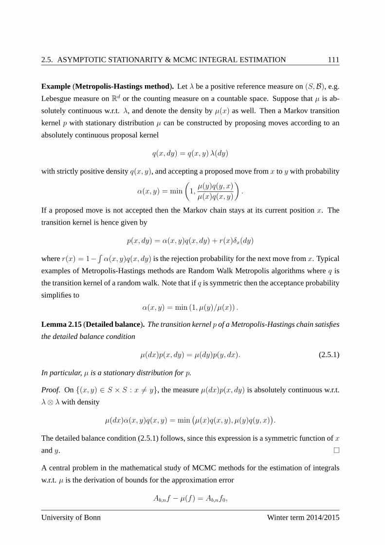
2.5. ASYMPTOTIC STATIONARITY & MCMC INTEGRAL ESTIMATION 111
Example (Metropolis-Hastings method). Let λ be a positive reference measure on(S,B), e.g.
Lebesgue measure onRd or the counting measure on a countable space. Suppose thatµ is ab-
solutely continuous w.r.t.λ, and denote the density byµ(x) as well. Then a Markov transition
kernelp with stationary distributionµ can be constructed by proposing moves according to an
absolutely continuous proposal kernel
q(x, dy) = q(x, y)λ(dy)
with strictly positive densityq(x, y), and accepting a proposed move fromx to y with probability
α(x, y) = min
(1,µ(y)q(y, x)
µ(x)q(x, y)
).
If a proposed move is not accepted then the Markov chain staysat its current positionx. The
transition kernel is hence given by
p(x, dy) = α(x, y)q(x, dy) + r(x)δx(dy)
wherer(x) = 1−´
α(x, y)q(x, dy) is the rejection probability for the next move fromx. Typical
examples of Metropolis-Hastings methods are Random Walk Metropolis algorithms whereq is
the transition kernel of a random walk. Note that ifq is symmetric then the acceptance probability
simplifies to
α(x, y) = min (1, µ(y)/µ(x)) .
Lemma 2.15(Detailed balance). The transition kernelp of a Metropolis-Hastings chain satisfies
the detailed balance condition
µ(dx)p(x, dy) = µ(dy)p(y, dx). (2.5.1)
In particular,µ is a stationary distribution forp.
Proof. On (x, y) ∈ S × S : x 6= y, the measureµ(dx)p(x, dy) is absolutely continuous w.r.t.
λ⊗ λ with density
µ(dx)α(x, y)q(x, y) = min(µ(x)q(x, y), µ(y)q(y, x)
).
The detailed balance condition (2.5.1) follows, since thisexpression is a symmetric function ofx
andy.
A central problem in the mathematical study of MCMC methods for the estimation of integrals
w.r.t. µ is the derivation of bounds for the approximation error
Ab,nf − µ(f) = Ab,nf0,
University of Bonn Winter term 2014/2015
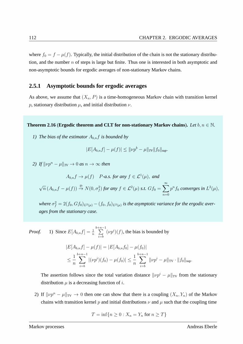
112 CHAPTER 2. ERGODIC AVERAGES
wheref0 = f − µ(f). Typically, the initial distribution of the chain is not thestationary distribu-
tion, and the numbern of steps is large but finite. Thus one is interested in both asymptotic and
non-asymptotic bounds for ergodic averages of non-stationary Markov chains.
2.5.1 Asymptotic bounds for ergodic averages
As above, we assume that(Xn, P ) is a time-homogeneous Markov chain with transition kernel
p, stationary distributionµ, and initial distributionν.
Theorem 2.16(Ergodic theorem and CLT for non-stationary Markov chains). Let b, n ∈ N.
1) The bias of the estimatorAb,nf is bounded by
|E[Ab,nf ]− µ(f)| ≤ ‖νpb − µ‖TV‖f0‖sup.
2) If ‖νpn − µ‖TV → 0 asn→ ∞ then
Ab,nf → µ(f) P -a.s. for anyf ∈ L1(µ), and
√n (Ab,nf − µ(f))
D→ N(0, σ2f ) for anyf ∈ L2(µ) s.t.Gf0 =
∞∑
n=0
pnf0 converges inL2(µ),
whereσ2f = 2(f0, Gf0)L2(µ) − (f0, f0)L2(µ) is the asymptotic variance for the ergodic aver-
ages from the stationary case.
Proof. 1) SinceE[Ab,nf ] =1n
b+n−1∑i=b
(νpi)(f), the bias is bounded by
|E[Ab,nf ]− µ(f)| = |E[Ab,nf0]− µ(f0)|
≤ 1
n
b+n−1∑
i=b
|(νpi)(f0)− µ(f0)| ≤1
n
b+n−1∑
i=b
‖νpi − µ‖TV · ‖f0‖sup.
The assertion follows since the total variation distance‖νpi − µ‖TV from the stationary
distributionµ is a decreasing function ofi.
2) If ‖νpn − µ‖TV → 0 then one can show that there is a coupling(Xn, Yn) of the Markov
chains with transition kernelp and initial distributionsν andµ such that the coupling time
T = infn ≥ 0 : Xn = Yn for n ≥ T
Markov processes Andreas Eberle
2.5. ASYMPTOTIC STATIONARITY & MCMC INTEGRAL ESTIMATION 113
is almost surely finite (Exercise). We can then approximateAb,nf by ergodic averages for
the stationary Markov chain(Yn):
Ab,nf =1
n
b+n−1∑
i=b
f(Yi) +1
n
b+n−1∑
i=b
(f(Xi)− f(Yi))1i<T.
The second sum is constant forb + n ≥ T , so 1n
times the sum converges almost surely to
zero, whereas the ergodic theorem and the central limit theorem apply to the first term on
the right hand side. This proves the assertion.
To apply the theorem in practice, bounds for the asymptotic variance are required. One possibility
for deriving such bounds is to estimate the contraction coefficient of the transition kernels on the
orthogonal complement
L20(µ) = f ∈ L2(µ) : µ(f) = 0
of the constants in the Hilbert spaceL2(µ). Indeed, let
γ(p) = ‖p‖L20(µ)→L2
0(µ)= sup
f⊥1
‖pf‖L2(µ)
‖f‖L2(µ)
denote the operator norm ofp onL20(µ). If
c :=∞∑
n=0
γ(pn) <∞ (2.5.2)
thenGf0 =∞∑n=0
pnf0 converges for anyf ∈ L2(µ), i.e., the asymptotic variancesσ2f exist, and
σ2f = 2(f0, Gf0)L2(µ) − (f0, f0)L2(µ) (2.5.3)
≤ (2c− 1)‖f0‖2L2(µ) = (2c− 1)Varµ(f).
A sufficient condition for (2.5.2) to hold isγ(p) < 1; in that case
c ≤∞∑
n=0
γ(p)n =1
1− γ(p)<∞ (2.5.4)
by multiplicativity of the operator norm.
Remark (Relation to spectral gap). By definition,
γ(p) = supf⊥1
(pf, pf)1/2
L2(µ)
(f, f)1/2
L2(µ)
= supf⊥1
(f, p∗pf)1/2
L2(µ)
(f, f)1/2
L2(µ)
= (p∗p|L20(µ)
)1/2,
University of Bonn Winter term 2014/2015
114 CHAPTER 2. ERGODIC AVERAGES
i.e., γ(p) is the spectral radius of the linear operatorp∗p restricted toL20(µ). Now suppose
that p satisfies the detailed balance condition w.r.t.µ. As remarked above, this is the case for
Metropolis-Hastings chains and random scan Gibbs samplers. Thenp is a self-adjoint linear
operator on the Hilbert spaceL20(µ). Therefore,
γ(p) = (p∗p|L20(µ)
)1/2 = (p|L20(µ)
) = supf⊥1
(f, pf)L2(µ)
(f, f)L2(µ)
, and
1− γ(p) = inff⊥1
(f, f − pf)L2(µ)
(f, f)L2(µ)
= Gap(L),
where thespectral gapGap(L) of the generatorL = p− I is defined by
Gap(L) = inff⊥1
(f,−Lf)L2(µ)
(f, f)L2(µ)
= inf spec(−L|L20(µ)
).
Gap(L) is the gap in the spectrum of−L between the eigenvalue0 corresponding to the constant
functions and the infimum of the spectrum on the complement ofthe constants. By (2.5.2) and
(2.5.3),2Gap(L)− 1 provides upper bound for the asymptotic variances in the symmetric case.
2.5.2 Non-asymptotic bounds for ergodic averages
For deriving non-asymptotic error bounds for estimates by ergodic averages we assume contrac-
tivity in an appropriate Kantorovich distance. Suppose that there exists a distanced on S, and
constantsα ∈ (0, 1) andσ ∈ R+ such that
(A1) W1d (νp, νp) ≤ αW1
d (ν, ν) for anyν, ν ∈ P(S), and
(A2) Varp(x,·)(f) ≤ σ2‖f‖2Lip(d) for anyx ∈ S and any Lipschitz continuous functionf : S → R.
Suppose that(Xn, Px) is a Markov chain with transition kernelp.
Lemma 2.17(Decay of correlations). If (A1) and (A2) hold, then the following non-asymptotic
bounds hold for anyn, k ∈ N and any Lipschitz continuous functionf : S → R:
VarPx [f(Xn)] ≤n−1∑
k=0
α2kσ2‖f‖2Lip(d), and (2.5.5)
|CovPx [f(Xn), f(Xn+k)]| ≤αk
1− α2σ2‖f‖2Lip(d). (2.5.6)
Markov processes Andreas Eberle
2.5. ASYMPTOTIC STATIONARITY & MCMC INTEGRAL ESTIMATION 115
Proof. The inequality (2.5.5) follows by induction onn. It holds true forn = 0, and if (2.5.5)
holds for somen ≥ 0 then
VarPx [f(Xn+1)] = Ex
[VarPx [f(Xn+1)|FX
n ]]+VarPx
[Ex[f(Xn+1)|FX
n ]]
= Ex
[Varp(Xn,·)(f)
]+VarPx
[(pf)(Xn)
]
≤ σ2‖f‖2Lip(d) +n−1∑
k=0
α2kσ2‖pf‖2Lip(d)
≤n∑
k=0
α2kσ2‖f‖2Lip(d)
by the Markov property and the assumptions (A1) and (A2). Noting thatn−1∑
k=0
α2k ≤ 1
1− α2for anyn ∈ N,
the bound (2.5.6) for the correlations follows from (2.5.5)since∣∣CovPx [f(Xn), f(Xn+k)]
∣∣ =∣∣CovPx
[f(Xn), (p
kf)(Xn)] ∣∣
≤ VarPx [f(Xn)]1/2 VarPx
[(pkf)(Xn)
]1/2
≤ 1
1− α2σ2‖f‖Lip(d)‖pkf‖Lip(d)
≤ αk
1− α2σ2‖f‖2Lip(d)
by Assumption (A1).
As a consequence of Lemma 2.17 we obtain a non-asymptotic upper bound for variances of
ergodic averages.
Theorem 2.18(Quantitative bounds for bias and variance of ergodic averages of non sta-
tionary Markov chains ). Suppose that (A1) and (A2) hold. Then the following upper bounds
hold for anyb, n ∈ N, any initial distributionν ∈ P(S), and any Lipschitz continuous function
f : S → R:
∣∣Eν [Ab,nf ]− µ(f)∣∣ ≤ 1
n
αb
1− αW1
d (ν, µ)‖f‖Lip(d), (2.5.7)
VarPν [Ab,nf ] ≤1
n‖f‖2Lip(d) ·
1
(1− α)2
(σ2 +
α2b
nVar(ν)
)(2.5.8)
whereµ is a stationary distribution for the transition kernelp, and
Var(ν) :=1
2
ˆ ˆ
d(x, y)2ν(dx)ν(dy).
University of Bonn Winter term 2014/2015
116 CHAPTER 2. ERGODIC AVERAGES
Proof. 1) By definition of the averaging operator,
Eν [Ab,nf ] =1
n
b+n−1∑
i=b
(νpi)(f), and thus
|Eν [Ab,nf ]− µ(f)| ≤ 1
n
b+n−1∑
i=b
|(νpi)(f)− µ(f)|
≤ 1
n
b+n−1∑
i=b
W1d (νp
i, µ) ‖f‖Lip(d) ≤1
n
b+n−1∑
i=b
αi W1d (ν, µ) ‖f‖Lip(d).
2) By the correlation bound in Lemma 2.17,
VarPx [Ab,nf ] =1
n2
b+n−1∑
i,j=b
CovPx [f(Xi), f(Xj)] ≤1
n2
b+n−1∑
i,j=b
α|i−j|
1− α2σ2 ‖f‖2Lip(d)
≤ 1
n
σ2
(1− α2)
(1 + 2
∞∑
k=1
αk
)‖f‖2Lip(d) =
1
n
σ2
(1− α)2‖f‖2Lip(d).
Therefore, for an arbitrary initial distributionν ∈ P(S),
VarPν [Ab,nf ] = Eν [VarPν [Ab,nf |X0]] + VarPν [Eν [Ab,nf |X0]]
=
ˆ
VarPx [Ab,nf ] ν(dx) + Varν
[1
n
b+n−1∑
i=b
pif
]
≤ 1
n
σ2
(1− α)2‖f‖2Lip(d) +
(1
n
b+n−1∑
i=b
Varν(pif)1/2
)2
.
The assertion now follows since
Varν(pif) ≤ 1
2‖pif‖2Lip(d)
¨
d(x, y)2ν(dx)ν(dy)
≤ α2i ‖f‖2Lip(d)Var(ν).
Markov processes Andreas Eberle
Chapter 3
Continuous time Markov processes,
generators and martingales
This chapter focuses on the connection between continuous-time Markov processes and their
generators. Throughout we assume that the state spaceS is a Polish space with Borelσ-algebra
B. Recall that a right-continuous stochastic process((Xt)t∈R+ , P ) that is adapted to a filtration
(Ft)t∈R+ is called asolution of the martingale problem for a family (Lt,A), t ∈ R+, of linear
operatorswith domainA ⊆ Fb(S) if and only if
M[f ]t = f(Xt)−
ˆ t
0
(Lsf)(Xs) ds (3.0.1)
is an(Ft) martingale for any functionf ∈ A. Here functionsf : S → R are extended trivially
to S ∪ ∆ by settingf(∆) := 0.
If ((Xt), P ) solves the martingale problem for((Lt),A) and the function(t, x) 7→ (Ltf)(x) is,
for example, continuous and bounded forf ∈ A, then
(Ltf)(Xt) = limh↓0
E
[f(Xt+h)− f(Xt)
h
∣∣∣∣Ft
](3.0.2)
is the expected rate of change off(Xt) in the next instant of time given the previous information.
In general, solutions of a martingale problem are not necessarily Markov processes, but it can
be shown under appropriate assumptions, that the strong Markov property follows from unique-
ness of solutions of the martingale problem with a given initial law, cf. Theorem 3.22. Now
suppose that for anyt ≥ 0 andx ∈ S, ((Xs)s≥t, P(t,x)) is an(Ft) Markov process with initial
117
118CHAPTER 3. CONTINUOUS TIME MARKOV PROCESSES, GENERATORS AND
MARTINGALES
valueXt = x P(t,x)-almost surely and transition function(ps,t)0≤s≤t that solves the martingale
problem above. Then for anyt ≥ 0 andx ∈ S,
(Ltf)(x) = limh↓0
Ex
[f(Xt+h)− f(Xt)
h
]= lim
h↓0
(pt,t+hf)(x)− f(x)
h
provided(t, x) 7→ (Ltf)(x) is continuous and bounded. This indicates that the infinitesimal gen-
erator of the Markov process at timet is an extension of the operator(Lt,A) - this fact will be
made precise in Section 3.4.
In this chapter we will mostly restrict ourselves to the time-homogeneous case. The time-
inhomogeneous case is nevertheless included implicitly since we may apply most results to the
time space processXt = (t0 + t,Xt0+t) that is always a time-homogeneous Markov process if
X is a Markov process w.r.t. some probability measure. In Section 3.3 we show how to realize
transition functions of time-homogeneous Markov processes as strongly continuous contraction
semigroups on appropriate Banach space of functions, and we establish the relation between
such semigroups and their generators. The connection to martingale problems is made in Section
3.4, and Section 3.5 indicates in a special situation how solutions of martingale problems can be
constructed from their generators by exploiting stabilityof the martingale problem under weak
convergence. Before turning to the general setup, Section 3.1 is devoted mainly to an explicit
construction of jump processes with finite jump intensitiesfrom their jump rates (i.e. from their
generators), and the derivation of forward and backward equations and the martingale problem
in this more concrete context. Section 3.2 briefly discussesthe application of Lyapunov function
techniques in continuous time.
3.1 Jump processes and diffusions
3.1.1 Jump processes with finite jump intensity
Let qt : S × S → [0,∞] be akernel of positive measure, i.e. x 7→ qt(x,A) is measurable and
A 7→ qt(x,A) is a positive measure.
Aim: Construct a pure jump process with instantaneous jump ratesqt(x, dy), i.e.
Pt,t+h(x,B) = qt(x,B) · h+ o(h) ∀ t ≥ 0, x ∈ S, B ⊆ S \ x measurable
Markov processes Andreas Eberle
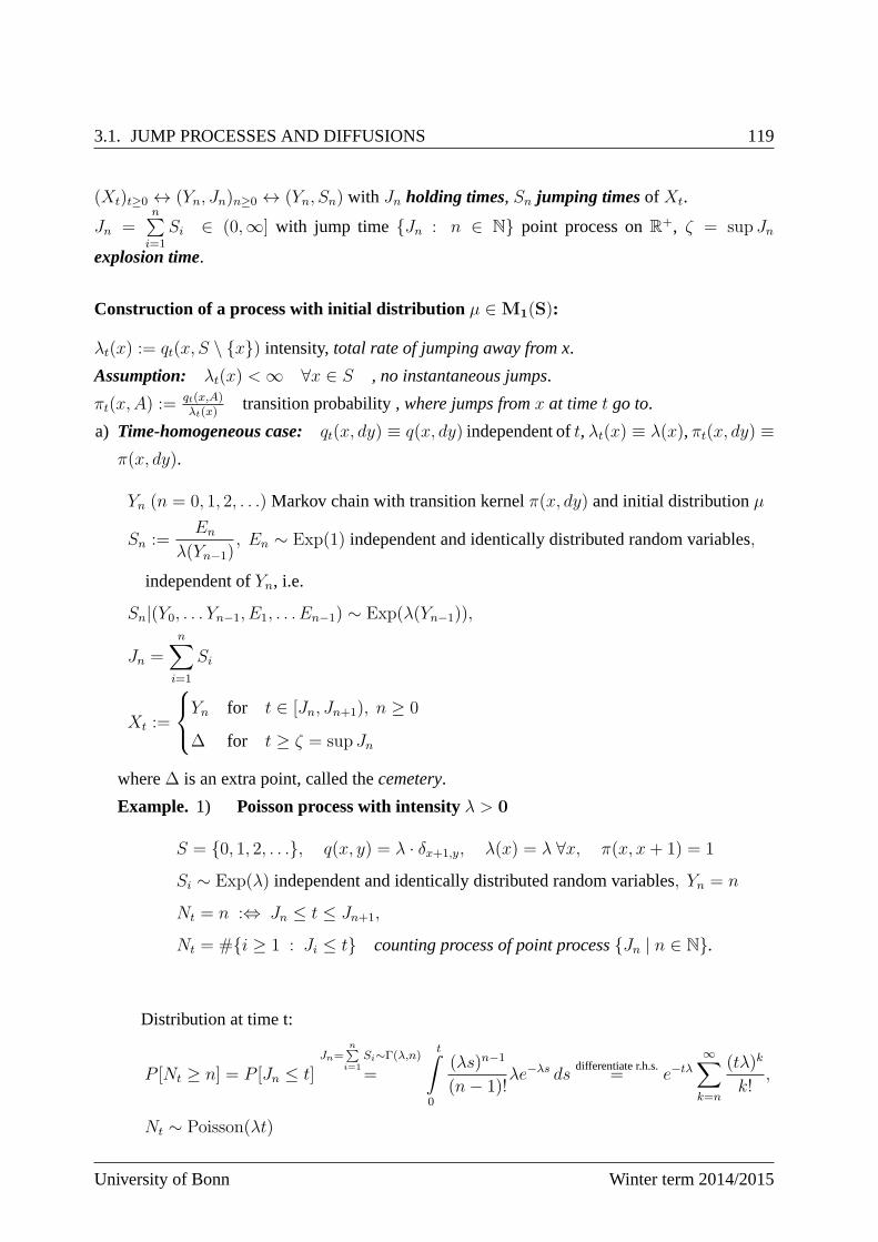
3.1. JUMP PROCESSES AND DIFFUSIONS 119
(Xt)t≥0 ↔ (Yn, Jn)n≥0 ↔ (Yn, Sn) with Jn holding times, Sn jumping timesof Xt.
Jn =n∑
i=1
Si ∈ (0,∞] with jump time Jn : n ∈ N point process onR+, ζ = sup Jn
explosion time.
Construction of a process with initial distribution µ ∈ M1(S):
λt(x) := qt(x, S \ x) intensity,total rate of jumping away from x.
Assumption: λt(x) <∞ ∀x ∈ S , no instantaneous jumps.
πt(x,A) :=qt(x,A)λt(x)
transition probability, where jumps fromx at timet go to.
a) Time-homogeneous case:qt(x, dy) ≡ q(x, dy) independent oft, λt(x) ≡ λ(x),πt(x, dy) ≡π(x, dy).
Yn (n = 0, 1, 2, . . .) Markov chain with transition kernelπ(x, dy) and initial distributionµ
Sn :=En
λ(Yn−1), En ∼ Exp(1) independent and identically distributed random variables,
independent ofYn, i.e.
Sn|(Y0, . . . Yn−1, E1, . . . En−1) ∼ Exp(λ(Yn−1)),
Jn =n∑
i=1
Si
Xt :=
Yn for t ∈ [Jn, Jn+1), n ≥ 0
∆ for t ≥ ζ = sup Jn
where∆ is an extra point, called thecemetery.
Example. 1) Poisson process with intensityλ > 0
S = 0, 1, 2, . . ., q(x, y) = λ · δx+1,y, λ(x) = λ ∀x, π(x, x+ 1) = 1
Si ∼ Exp(λ) independent and identically distributed random variables, Yn = n
Nt = n :⇔ Jn ≤ t ≤ Jn+1,
Nt = #i ≥ 1 : Ji ≤ t counting process of point processJn | n ∈ N.
Distribution at time t:
P [Nt ≥ n] = P [Jn ≤ t]Jn=
n∑
i=1Si∼Γ(λ,n)
=
tˆ
0
(λs)n−1
(n− 1)!λe−λs ds
differentiate r.h.s.= e−tλ
∞∑
k=n
(tλ)k
k!,
Nt ∼ Poisson(λt)
University of Bonn Winter term 2014/2015
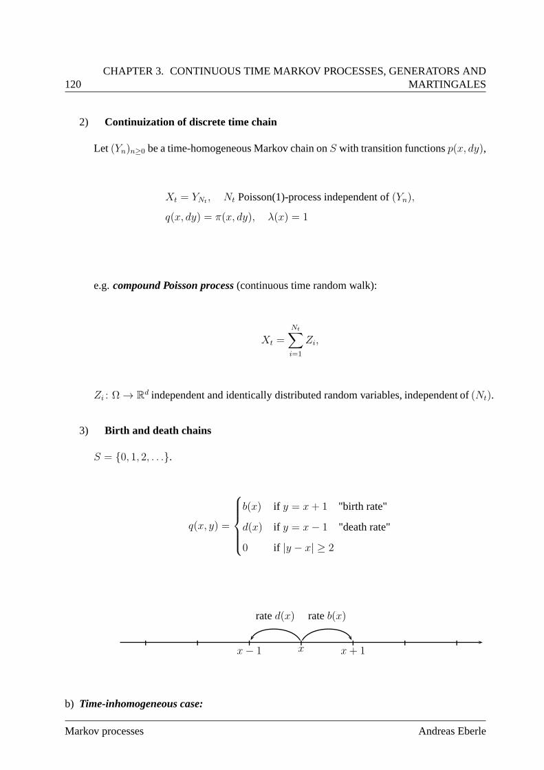
120CHAPTER 3. CONTINUOUS TIME MARKOV PROCESSES, GENERATORS AND
MARTINGALES
2) Continuization of discrete time chain
Let (Yn)n≥0 be a time-homogeneous Markov chain onS with transition functionsp(x, dy),
Xt = YNt , Nt Poisson(1)-process independent of(Yn),
q(x, dy) = π(x, dy), λ(x) = 1
e.g.compound Poisson process(continuous time random walk):
Xt =Nt∑
i=1
Zi,
Zi : Ω → Rd independent and identically distributed random variables, independent of(Nt).
3) Birth and death chains
S = 0, 1, 2, . . ..
q(x, y) =
b(x) if y = x+ 1 "birth rate"
d(x) if y = x− 1 "death rate"
0 if |y − x| ≥ 2
| | | | | | |xx− 1 x+ 1
rateb(x)rated(x)
b) Time-inhomogeneous case:
Markov processes Andreas Eberle
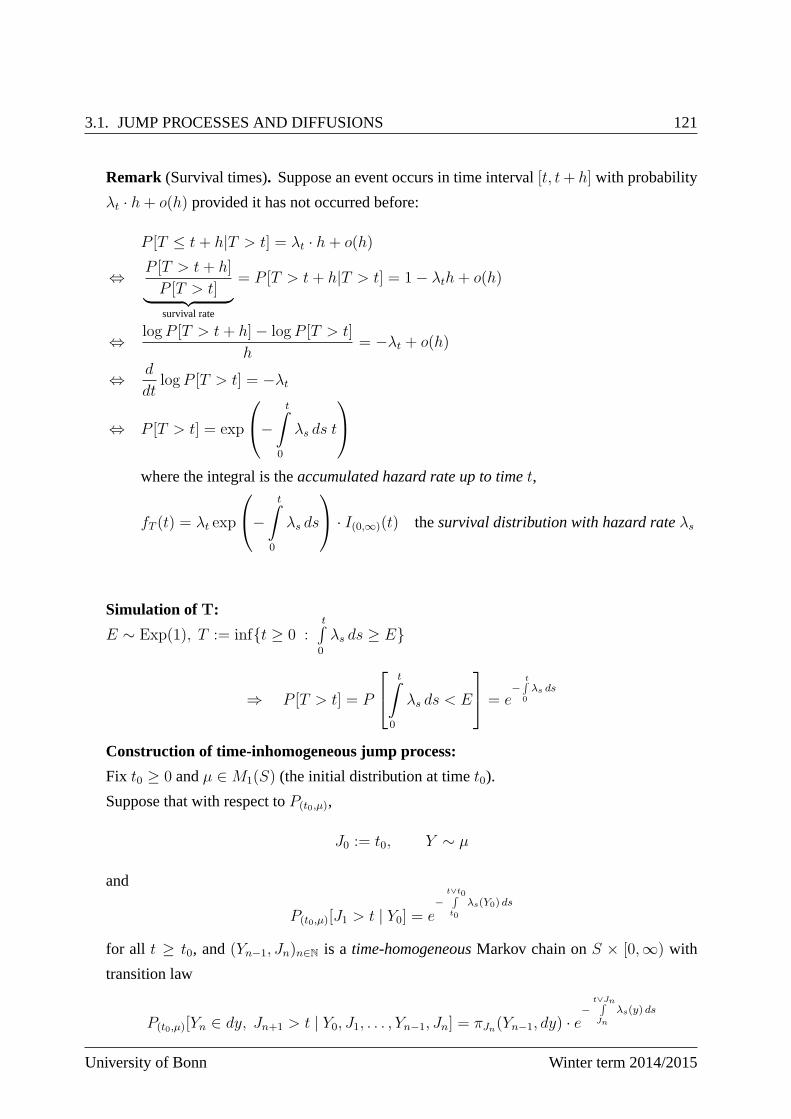
3.1. JUMP PROCESSES AND DIFFUSIONS 121
Remark (Survival times). Suppose an event occurs in time interval[t, t+ h] with probability
λt · h+ o(h) provided it has not occurred before:
P [T ≤ t+ h|T > t] = λt · h+ o(h)
⇔ P [T > t+ h]
P [T > t]︸ ︷︷ ︸survival rate
= P [T > t+ h|T > t] = 1− λth+ o(h)
⇔ logP [T > t+ h]− logP [T > t]
h= −λt + o(h)
⇔ d
dtlogP [T > t] = −λt
⇔ P [T > t] = exp
−
tˆ
0
λs ds t
where the integral is theaccumulated hazard rate up to timet,
fT (t) = λt exp
−
tˆ
0
λs ds
· I(0,∞)(t) thesurvival distribution with hazard rateλs
Simulation of T:
E ∼ Exp(1), T := inft ≥ 0 :t
0
λs ds ≥ E
⇒ P [T > t] = P
tˆ
0
λs ds < E
= e
−t
0
λs ds
Construction of time-inhomogeneous jump process:
Fix t0 ≥ 0 andµ ∈M1(S) (the initial distribution at timet0).
Suppose that with respect toP(t0,µ),
J0 := t0, Y ∼ µ
and
P(t0,µ)[J1 > t | Y0] = e−
t∨t0´
t0
λs(Y0) ds
for all t ≥ t0, and(Yn−1, Jn)n∈N is a time-homogeneousMarkov chain onS × [0,∞) with
transition law
P(t0,µ)[Yn ∈ dy, Jn+1 > t | Y0, J1, . . . , Yn−1, Jn] = πJn(Yn−1, dy) · e−
t∨Jn´
Jn
λs(y) ds
University of Bonn Winter term 2014/2015
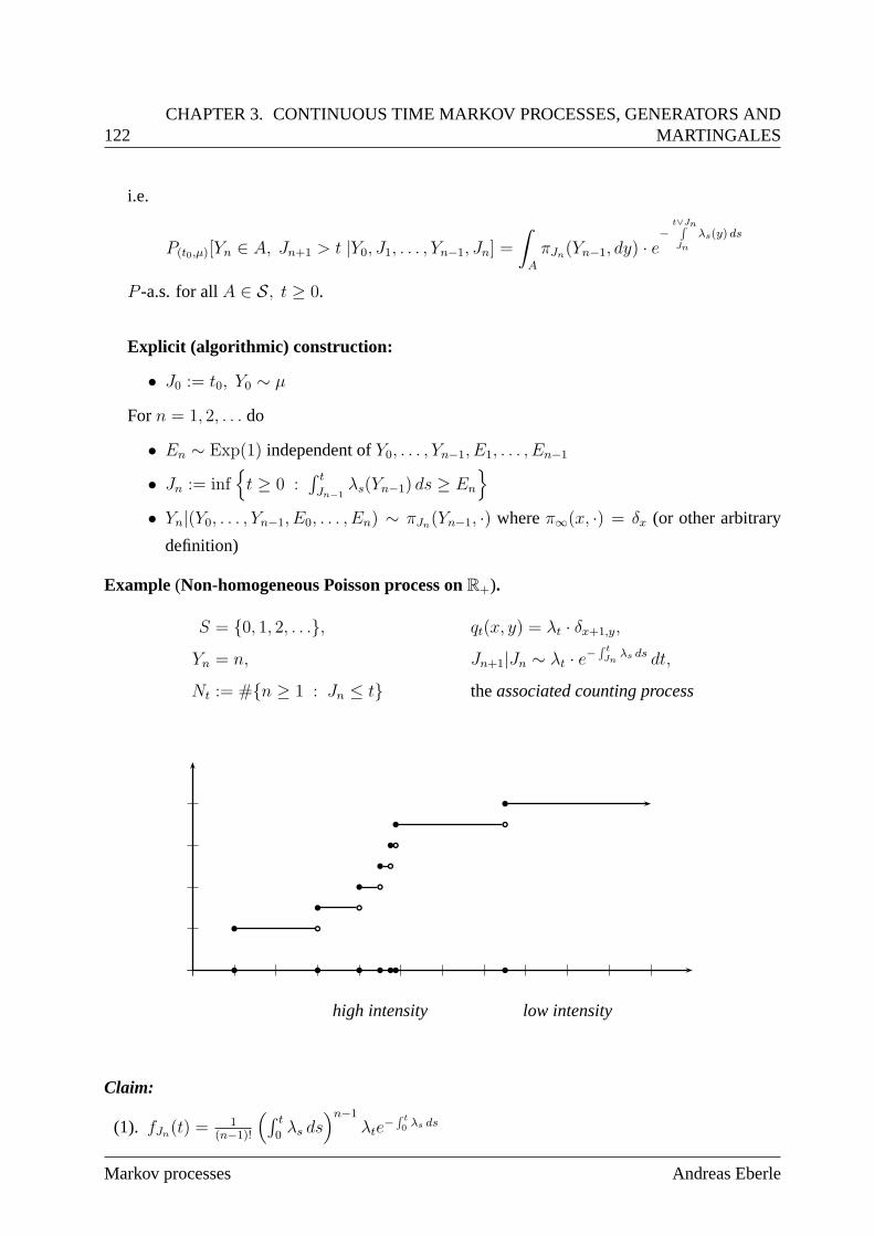
122CHAPTER 3. CONTINUOUS TIME MARKOV PROCESSES, GENERATORS AND
MARTINGALES
i.e.
P(t0,µ)[Yn ∈ A, Jn+1 > t |Y0, J1, . . . , Yn−1, Jn] =
ˆ
A
πJn(Yn−1, dy) · e−
t∨Jn´
Jn
λs(y) ds
P -a.s. for allA ∈ S, t ≥ 0.
Explicit (algorithmic) construction:
• J0 := t0, Y0 ∼ µ
Forn = 1, 2, . . . do
• En ∼ Exp(1) independent ofY0, . . . , Yn−1, E1, . . . , En−1
• Jn := inft ≥ 0 :
´ t
Jn−1λs(Yn−1) ds ≥ En
• Yn|(Y0, . . . , Yn−1, E0, . . . , En) ∼ πJn(Yn−1, ·) whereπ∞(x, ·) = δx (or other arbitrary
definition)
Example (Non-homogeneous Poisson process onR+).
S = 0, 1, 2, . . ., qt(x, y) = λt · δx+1,y,
Yn = n, Jn+1|Jn ∼ λt · e−´ tJn
λs ds dt,
Nt := #n ≥ 1 : Jn ≤ t theassociated counting process
b b b b b b b
high intensity low intensity
Claim:
(1). fJn(t) =1
(n−1)!
(´ t
0λs ds
)n−1
λte−´ t0 λs ds
Markov processes Andreas Eberle
3.1. JUMP PROCESSES AND DIFFUSIONS 123
(2). Nt ∼ Poisson(´ t
0λs ds
)
Proof. (1). By induction:
fJn+1(t) =
tˆ
0
fJn−1|Jn(t|r)fJn(r) dr
=
tˆ
0
λte−´ tr λs ds
1
(n− 1)!
rˆ
0
λs ds
n−1
λre−´ r0 λs ds dr = . . .
(2). P [Nt ≥ n] = P [Jn ≤ t]
Remark. In general,(Yn) is not a Markov chain. However:
(1). (Yn−1, Jn) is a Markov chain with respect toGn = σ(Y0, . . . , Yn−1, E1, . . . , En) with tran-
sition functions
p ((x, s), dydt) = πs(x, dy)λt(y) · e−´ ts λr(y) drI(s,∞)(t) dt
(2). (Jn, Yn) is a Markov chain with respect toG = σ(Y0, . . . , Yn, E1, . . . , En) with transition
functions
p ((x, s), dtdy) = λt(x) · e−´ ts λr(x) drI(s,∞)(t)πt(x, dy)
Remark. (1). Jn strictly increasing.
(2). Jn = ∞ ∀n,m is possible Xt absorbed in stateYn−1.
(3). sup Jn <∞ explosion in finite time
(4). s < ζ = Xs 6= ∆ ∈ Fs no explosion before times.
3.1.2 Markov property
Ks := minn : Jn > s first jump after times. Stopping time with respect to
Gn = σ (E1, . . . , En, Y0, . . . , Yn−1),
Ks <∞ = s < ζ
University of Bonn Winter term 2014/2015
124CHAPTER 3. CONTINUOUS TIME MARKOV PROCESSES, GENERATORS AND
MARTINGALES
Lemma (Memoryless property). Lets ≥ t0. Then for allt ≥ s,
P(t0,µ) [JKs > t ∩ s < ζ | Fs] = e−´ ts λr(Xs) dr P -a.s. ons < ζ
i.e.
P(t0,µ) [JKs > t ∩ s < ζ ∩ A] = E(t0,µ)
[e−´ ts λr(Xs) dr ; A ∩ s < ζ
]∀A ∈ Fs
Remark. The assertion is a restricted form of the Markov property in continuous time: The
conditional distribution with respect toP(t0,µ) of JKs givenFs coincides with the distribution of
J1 with respect toP(s,Xs).
Proof.
A ∈ Fs(Ex.)⇒ A ∩ Ks = n ∈ σ (J0, Y0, . . . , Jn−1, Yn−1) = Gn−1
⇒ P [JKs > t ∩ A ∩ Ks = n] = E[P [Jn > t | Gn−1] ; A ∩ Ks = n
]
where
P [Jn > t | Gn−1] = exp
−
tˆ
Jn−1
λr(Yn−1) dr
= exp
−
tˆ
s
λr(Yn−1︸︷︷︸=Xs
) dr
· P [Jn > s | Gn−1],
hence we get
P [Jn > t | Gn−1] = E[e−´ ts λr(Xs) dr ; A ∩ Ks = n ∩ Jn > s
]∀n ∈ N
whereA ∩ Ks = n ∩ Jn > s = A ∩ Ks = n.
Summing overn gives the assertion since
s < ζ =⋃
n∈NKs = n.
Foryn ∈ S, tn ∈ [0,∞] strictly increasing define
x := Φ ((tn, yn)n=0,1,2,...) ∈ PC ([t0,∞), S∪∆)
by
xt :=
Yn for tn ≤ t < tn+1 , n ≥ 0
∆ for t ≥ sup tn
Markov processes Andreas Eberle
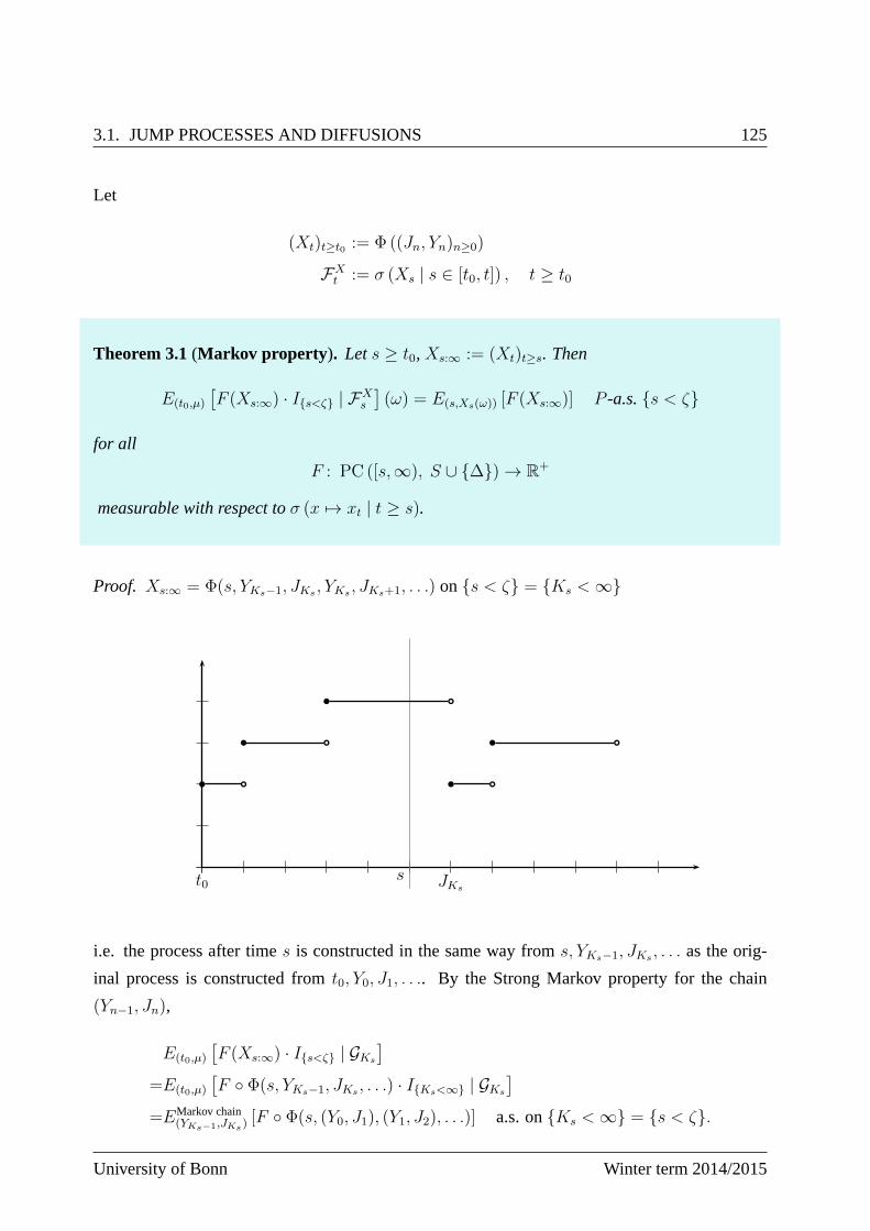
3.1. JUMP PROCESSES AND DIFFUSIONS 125
Let
(Xt)t≥t0 := Φ ((Jn, Yn)n≥0)
FXt := σ (Xs | s ∈ [t0, t]) , t ≥ t0
Theorem 3.1(Markov property ). Lets ≥ t0,Xs:∞ := (Xt)t≥s. Then
E(t0,µ)
[F (Xs:∞) · Is<ζ | FX
s
](ω) = E(s,Xs(ω)) [F (Xs:∞)] P -a.s.s < ζ
for all
F : PC ([s,∞), S ∪ ∆) → R+
measurable with respect toσ (x 7→ xt | t ≥ s).
Proof. Xs:∞ = Φ(s, YKs−1, JKs , YKs , JKs+1, . . .) ons < ζ = Ks <∞
t0 s JKs
i.e. the process after times is constructed in the same way froms, YKs−1, JKs , . . . as the orig-
inal process is constructed fromt0, Y0, J1, . . .. By the Strong Markov property for the chain
(Yn−1, Jn),
E(t0,µ)
[F (Xs:∞) · Is<ζ | GKs
]
=E(t0,µ)
[F Φ(s, YKs−1, JKs , . . .) · IKs<∞ | GKs
]
=EMarkov chain(YKs−1,JKs )
[F Φ(s, (Y0, J1), (Y1, J2), . . .)] a.s. onKs <∞ = s < ζ.
University of Bonn Winter term 2014/2015
126CHAPTER 3. CONTINUOUS TIME MARKOV PROCESSES, GENERATORS AND
MARTINGALES
SinceFs ⊆ GKs , we obtain by the projectivity of the conditional expectation,
E(t0,µ)
[F (Xs:∞) · Is<ζ | Fs
]
=E(t0,µ)
[EMarkov chain
(Xs,JKs )
[F Φ(s, (Y0, J1), . . .) · Is<ζ | Fs
]]
taking into account that the conditional distribution given GKs is 0 ons ≥ ζ and thatYKs−1 =
Xs.
Here the conditional distribution ofJKs ist k(Xs, ·), by Lemma 3.1.2
k(x, dt) = λt(x) · e−´ ts λr(x) dr · I(s,∞)(t) dt
hence
E(t0,µ)
[F (Xs:∞) · Is<ζ | Fs
]= EMarkov chain
(Xs,k(Xs,·)) [F Φ(. . .)] a.s. ons < ζ
Herek(Xs, ·) is the distribution ofJ1 with respect toPs,Xs , hence we obtain
E(t0,µ)
[F (Xs:∞) · Is<ζ | Fs
]= E(s,Xs) [F (Φ(s, Y0, J1, . . .))]
= E(s,Xs) [F (Xs:∞)]
Example (Non-homogeneous Poisson process). A non-homogeneous Poisson process(Nt)t≥0
with intensityλt has independent increments with distribution
Nt −Ns ∼ Poisson
tˆ
s
λr dr
Proof:
P[Nt −Ns ≥ k | FN
s
] MP= P(s,Ns) [Nt −Ns ≥ k] = P(s,Ns) [Jk ≤ t]
as above= Poisson
tˆ
s
λr dr
(k, k + 1, . . .) .
HenceNt −Ns independent ofFNs andPoisson
(´ t
sλr dr
)distributed.
Markov processes Andreas Eberle
3.1. JUMP PROCESSES AND DIFFUSIONS 127
3.1.3 Generator and backward equation
Definition. Theinfinitesimal generator(or intensity matrix, kernel) of a Markov jump process
at time t is defined by
Lt(x, dy) = qt(x, dy)− λt(x)δx(dy)
i.e.
(Ltf)(x) = (qtf)(x)− λt(x)f(x)
=
ˆ
qt(x, dy) · (f(y)− f(x))
for all bounded and measurablef : S → R.
Remark. (1). Lt is a linear operator on functionsf : S → R.
(2). If S is discrete,Lt is a matrix,Lt(x, y) = qt(x, y) − λt(x)δ(x, y). This matrix is called
Q-Matrix.
Theorem 3.2(Integrated backward equation). (1). UnderP(t0,µ), (Xt)t≥t0 is a Markov jump
process with initial distributionXt0 ∼ µ and transition probabilities
ps,t (x,B) = P(s,x) [Xt ∈ B] (0 ≤ s ≤ t, x ∈ S, B ∈ S)
satisfying the Chapman-Kolmogorov equationsps,tpt,u = ps,u ∀ 0 ≤ s ≤ t ≤ u.
(2). Theintegrated backward equation
ps,t(x,B) = e−´ ts λr(x) drδx(B) +
tˆ
s
e−´ rs λu(x) du(qrpr,t)(x,B) dr (3.1.1)
holds for all0 ≤ s ≤ t , x ∈ S andB ∈ S.
(3). If t 7→ λt(x) is continuous for allx ∈ S, then
(ps,s+hf)(x) = (1− λs(x) · h)f(x) + h · (qsf)(x) + o(h) (3.1.2)
holds for all s ≥ 0 , x ∈ S and bounded functionsf : → R such thatt 7→ (qtf)(x) is
continuous.
University of Bonn Winter term 2014/2015
128CHAPTER 3. CONTINUOUS TIME MARKOV PROCESSES, GENERATORS AND
MARTINGALES
Remark. (1). (3.1.2) shows that(Xt) is the continuous time Markov chain with intensities
λt(x) and transition ratesqt(x, dy).
(2). If ζ = sup Jn is finite with strictly positive probability, then there areother possible con-
tinuations ofXt after the explosion timeζ.
non-uniqueness.
The constructed process is called theminimal chain for the given jump rates, since its
transition probabilitiespt(x,B) , B ∈ S are minimal for all continuations, cf. below.
(3). The integrated backward equation extends to bounded functionsf : S → R
(ps,tf)(x) = e−´ ts λr(x) drf(x) +
tˆ
s
e−´ rs λu(x) du(qrpr,tf)(x) dr (3.1.3)
Proof. (1). By the Markov property,
P(t0,µ)
[Xt ∈ B|FX
s
]= P(s,Xs) [Xt ∈ B] = ps,t(Xs, B) a.s.
sinceXt ∈ B ⊆ t < ζ ⊆ s < ζ for all B ∈ S and0 ≤ s ≤ t.
Thus((Xt)t≥t0 , P(t0,µ)
)is a Markov jump process with transition kernelsps,t. Since this
holds for any initial condition, the Chapman-Kolmogorov equations
(ps,tpt,uf)(x) = (ps,uf)(x)
are satisfied for allx ∈ S , 0 ≤ s ≤ t ≤ u andf : S → R.
(2). First step analysis: Condition onG1 = σ(J0, Y0, J1, Y1):
SinceXt = Φt(J0, Y0, J1, Y1, J2, Y2, . . .), the Markov property of(Jn, Yn) implies
P(s,x)
[Xt ∈ B|G1
](ω) = P(J1(ω),Y1(ω)) [Φt(s, x, J0, Y0, J1, Y1, . . .) ∈ B]
On the right side, we see that
Φt(s, x, J0, Y0, J1, Y1, . . .) =
x if t < J1(ω)
Φt(J0, Y0, J1, Y1, . . .) if t ≥ J1(ω)
and hence
P(s,x)
[Xt ∈ B|G1
](ω) = δx(B) · It<J1(ω) + P(J1(ω),Y1(ω))[Xt ∈ B] · It≥J1(ω)
Markov processes Andreas Eberle
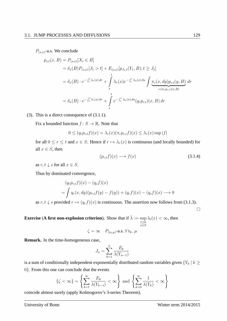
3.1. JUMP PROCESSES AND DIFFUSIONS 129
P(s,x)-a.s. We conclude
ps,t(x,B) = P(s,x)[Xt ∈ B]
= δx(B)P(s,x)[J1 > t] + E(s,x)[pJ1,t(Y1, B); t ≥ J1]
= δx(B) · e−´ ts λr(x) dr +
tˆ
s
λr(x)e−´ rs λu(x) du
ˆ
πr(x, dy)pr,t(y,B)︸ ︷︷ ︸=(πrpr,t)(x,B)
dr
= δx(B) · e−´ ts λr(x) dr +
tˆ
s
e−´ rs λu(x) du(qrpr,t)(x,B) dr
(3). This is a direct consequence of (3.1.1).
Fix a bounded functionf : S → R. Note that
0 ≤ (qrpr,tf)(x) = λr(x)(πrpr,tf)(x) ≤ λr(x) sup |f |
for all 0 ≤ r ≤ t andx ∈ S. Hence ifr 7→ λr(x) is continuous (and locally bounded) for
all x ∈ S, then
(pr,tf)(x) −→ f(x) (3.1.4)
asr, t ↓ s for all x ∈ S.
Thus by dominated convergence,
(qrpr,tf)(x)− (qsf)(x)
=
ˆ
qr(x, dy)(pr,tf(y)− f(y)) + (qrf)(x)− (qsf)(x) −→ 0
asr, t ↓ s providedr 7→ (qrf)(x) is continuous. The assertion now follows from (3.1.3).
Exercise(A first non-explosion criterion). Show that ifλ := supt≥0x∈S
λt(x) <∞, then
ζ = ∞ P(t0,µ)-a.s.∀ t0, µ
Remark. In the time-homogeneous case,
Jn =n∑
k=1
Ek
λ(Yn−1)
is a sum of conditionally independent exponentially distributed random variables givenYk | k ≥0. From this one can conclude that the events
ζ <∞ =
∞∑
k=1
Ek
λ(Yk−1)<∞
and
∞∑
k=0
1
λ(Yk)<∞
coincide almost surely (apply Kolmogorov’s 3-series Theorem).
University of Bonn Winter term 2014/2015
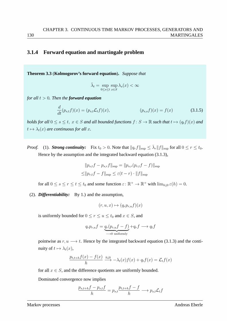
130CHAPTER 3. CONTINUOUS TIME MARKOV PROCESSES, GENERATORS AND
MARTINGALES
3.1.4 Forward equation and martingale problem
Theorem 3.3(Kolmogorov’s forward equation). Suppose that
λt = sup0≤s≤t
supx∈S
λs(x) <∞
for all t > 0. Then theforward equation
d
dt(ps,tf)(x) = (ps,tLtf)(x), (ps,sf)(x) = f(x) (3.1.5)
holds for all0 ≤ s ≤ t, x ∈ S and all bounded functionsf : S → R such thatt 7→ (qtf)(x) and
t 7→ λt(x) are continuous for allx.
Proof. (1). Strong continuity: Fix t0 > 0. Note that‖qrf‖sup ≤ λr‖f‖sup for all 0 ≤ r ≤ t0.
Hence by the assumption and the integrated backward equation (3.1.3),
‖ps,tf − ps,rf‖sup = ‖ps,r(pr,tf − f)‖sup≤‖pr,tf − f‖sup ≤ ε(t− r) · ‖f‖sup
for all 0 ≤ s ≤ r ≤ t ≤ t0 and some functionε : R+ → R+ with limh↓0 ε(h) = 0.
(2). Differentiability: By 1.) and the assumption,
(r, u, x) 7→ (qrpr,uf)(x)
is uniformly bounded for0 ≤ r ≤ u ≤ t0 andx ∈ S, and
qrpr,uf = qr(pr,uf − f)︸ ︷︷ ︸−→0 uniformly
+qrf −→ qtf
pointwise asr, u −→ t. Hence by the integrated backward equation (3.1.3) and the conti-
nuity of t 7→ λt(x),
pt,t+hf(x)− f(x)
h
h↓0−→ −λt(x)f(x) + qtf(x) = Ltf(x)
for all x ∈ S, and the difference quotients are uniformly bounded.
Dominated convergence now implies
ps,t+hf − ps,tf
h= ps,t
pt,t+hf − f
h−→ ps,tLtf
Markov processes Andreas Eberle
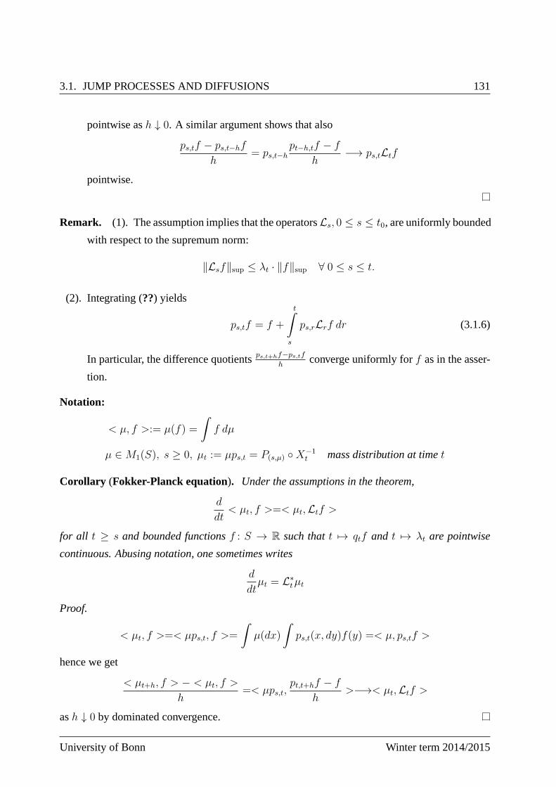
3.1. JUMP PROCESSES AND DIFFUSIONS 131
pointwise ash ↓ 0. A similar argument shows that also
ps,tf − ps,t−hf
h= ps,t−h
pt−h,tf − f
h−→ ps,tLtf
pointwise.
Remark. (1). The assumption implies that the operatorsLs, 0 ≤ s ≤ t0, are uniformly bounded
with respect to the supremum norm:
‖Lsf‖sup ≤ λt · ‖f‖sup ∀ 0 ≤ s ≤ t.
(2). Integrating (??) yields
ps,tf = f +
tˆ
s
ps,rLrf dr (3.1.6)
In particular, the difference quotientsps,t+hf−ps,tf
hconverge uniformly forf as in the asser-
tion.
Notation:
< µ, f >:= µ(f) =
ˆ
f dµ
µ ∈M1(S), s ≥ 0, µt := µps,t = P(s,µ) X−1t mass distribution at timet
Corollary (Fokker-Planck equation). Under the assumptions in the theorem,
d
dt< µt, f >=< µt,Ltf >
for all t ≥ s and bounded functionsf : S → R such thatt 7→ qtf and t 7→ λt are pointwise
continuous. Abusing notation, one sometimes writes
d
dtµt = L∗
tµt
Proof.
< µt, f >=< µps,t, f >=
ˆ
µ(dx)
ˆ
ps,t(x, dy)f(y) =< µ, ps,tf >
hence we get
< µt+h, f > − < µt, f >
h=< µps,t,
pt,t+hf − f
h>−→< µt,Ltf >
ash ↓ 0 by dominated convergence.
University of Bonn Winter term 2014/2015
132CHAPTER 3. CONTINUOUS TIME MARKOV PROCESSES, GENERATORS AND
MARTINGALES
Remark. (Important! )
P(s,µ)[ζ <∞] > 0
⇒ < µt, 1 >= µt(S) < 1 for larget
hence the Fokker-Planck equation doesnot hold forf ≡ 1:
< µt, 1 >︸ ︷︷ ︸<1
< < µ, 1 >︸ ︷︷ ︸=1
+
tˆ
0
< µs,Ls1 > ds
whereLs1 = 0.
Example. Birth process onS = 0, 1, 2, . . .
q(i, j) =
b(i) if j = i+ 1
0 else
π(i, j) = δi+1,j ,
Yn = n,
Sn = Jn − Jn−1 ∼ Exp(b(n− 1)) independent,
ζ = sup Jn =∞∑
n=1
Sn <∞ ⇐⇒∞∑
n=1
b(n)n−1 <∞
In this case, Fokker-Planck does not hold.
The question whether one can extend the forward equation to unbounded jump rates leads to the
martingale problem.
Definition. A Markov process(Xt, P(s,x) | 0 ≤ s ≤ t, x ∈ S) is called non-explosive(or
conservative) if and only ifζ = ∞ P(s,x)-a.s. for alls, x.
Now we consider again the minimal jump process(Xt, P(t0,µ)) constructed above. A function
f : [0,∞)× S → R
(t, x) 7→ ft(x)
is calledlocally boundedif and only if there exists an increasing sequence of open subsetsBn ⊆S such thatS =
⋃Bn, and
supx∈Bn0≤s≤t
|fs(x)| <∞
for all t > 0, n ∈ N.
The following theorem gives a probabilistic form of Kolmogorov’s forward equation:
Markov processes Andreas Eberle
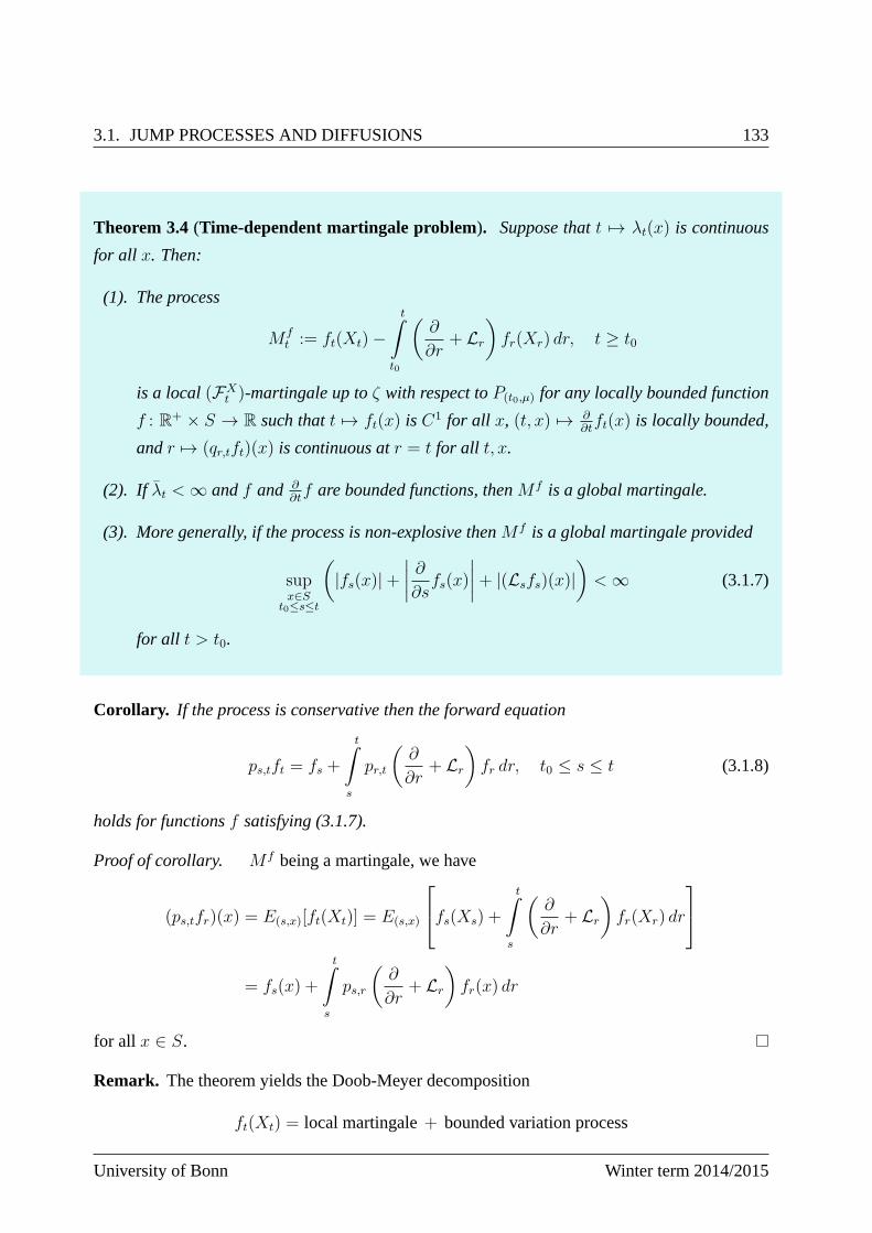
3.1. JUMP PROCESSES AND DIFFUSIONS 133
Theorem 3.4(Time-dependent martingale problem). Suppose thatt 7→ λt(x) is continuous
for all x. Then:
(1). The process
M ft := ft(Xt)−
tˆ
t0
(∂
∂r+ Lr
)fr(Xr) dr, t ≥ t0
is a local(FXt )-martingale up toζ with respect toP(t0,µ) for any locally bounded function
f : R+ × S → R such thatt 7→ ft(x) isC1 for all x, (t, x) 7→ ∂∂tft(x) is locally bounded,
andr 7→ (qr,tft)(x) is continuous atr = t for all t, x.
(2). If λt <∞ andf and ∂∂tf are bounded functions, thenM f is a global martingale.
(3). More generally, if the process is non-explosive thenM f is a global martingale provided
supx∈S
t0≤s≤t
(|fs(x)|+
∣∣∣∣∂
∂sfs(x)
∣∣∣∣+ |(Lsfs)(x)|)<∞ (3.1.7)
for all t > t0.
Corollary. If the process is conservative then the forward equation
ps,tft = fs +
tˆ
s
pr,t
(∂
∂r+ Lr
)fr dr, t0 ≤ s ≤ t (3.1.8)
holds for functionsf satisfying (3.1.7).
Proof of corollary. M f being a martingale, we have
(ps,tfr)(x) = E(s,x)[ft(Xt)] = E(s,x)
fs(Xs) +
tˆ
s
(∂
∂r+ Lr
)fr(Xr) dr
= fs(x) +
tˆ
s
ps,r
(∂
∂r+ Lr
)fr(x) dr
for all x ∈ S.
Remark. The theorem yields the Doob-Meyer decomposition
ft(Xt) = local martingale+ bounded variation process
University of Bonn Winter term 2014/2015
134CHAPTER 3. CONTINUOUS TIME MARKOV PROCESSES, GENERATORS AND
MARTINGALES
Remark. (1). Time-homogeneous case:
If h is an harmonic function, i.e.Lh = 0, thenh(Xt) is a martingale
(2). In general:
If ht is space-time harmonic, i.e. ∂∂tht+Ltht = 0, thenh(Xt) is a martingale. In particular,
(ps,tf)(Xt), (t ≥ s) is a martingale for all bounded functionsf .
(3). If ht is superharmonic (orexcessive), i.e. ∂∂tht+Ltht ≤ 0, thenht(Xt) is a supermartingale.
In particular,E[ht(Xt)] is decreasing
stochastic Lyapunov function, stability criteria
e.g.
ht(x) = e−tch(tc), Lth ≤ ch
Proof of theorem. 2. Similarly to the derivation of the forward equation, one shows that the
assumption implies
∂
∂t(ps,tft)(x) = (ps,tLtft) (x) +
(ps,t
∂
∂tft
)(x) ∀ x ∈ S,
or, in a integrated form,
ps,tft = fs +
tˆ
s
ps,r
(∂
∂r+ Lr
)fr dr
for all 0 ≤ s ≤ t. Hence by the Markov property, fort0 ≤ s ≤ t,
E(t0,µ)[ft(Xt)− fs(Xs) | FXs ]
=E(s,Xs)[ft(Xt)− fs(Xs)] = (ps,tft)(Xs)− fs(Xs)
=
tˆ
s
(ps,r
(∂
∂r+ Lr
)fr
)(Xs) dr
=E(t0,µ)
tˆ
s
(∂
∂r+ Lr
)fr(Xr) dr | FX
r
,
because all the integrands are uniformly bounded.
1. Fork ∈ N let
q(k)t (x,B) := (λt(x) ∧ k) · πt(x,B)
Markov processes Andreas Eberle
3.1. JUMP PROCESSES AND DIFFUSIONS 135
denote the jump rates for the processX(k)t with the same transition probabilities asXt and
jump rates cut off atk. By the construction above, the processX(k)t , k ∈ N, andXt can be
realized on the same probability space in such a way that
X(k)t = Xt a.s. ont < Tk
where
Tk := inf t ≥ 0 : λt(Xt) ≥ k, Xt /∈ Bk
for an increasing sequenceBk of open subsets ofS such thatf and ∂∂tf are bounded on
[0, t] × Bk for all t, k andS =⋃Bk. Sincet 7→ λt(Xt) is piecewise continuous and the
jump rates do not accumulate beforeζ, the function is locally bounded on[0, ζ). Hence
Tk ր ζ a.s. ask → ∞
By the theorem above,
M f,kt = ft(X
(k)t )−
tˆ
t0
(∂
∂r+ L(k)
r
)fr(X
(k)r ) dr, t ≥ t0,
is a martingale with respect toP(t0,µ), which coincides a.s. withM ft for t < Tk. HenceM f
t
is a local martingale up toζ = supTk.
3. If ζ = supTk = ∞ a.s. andf satisfies (3.1.7), then(M ft )t≥0 is a bounded local martingale,
and hence, by dominated convergence, a martingale.
3.1.5 Diffusion processes
A broad class of diffusion processes onRn can be constructed by stochastic analysis meth-
ods. Suppose that((Bt)t≥0, P ) is a Brownian motion with values inRn for somen ∈ N, and
((Xt)t<ζ , P ) is a solution to an Itô stochastic differential equation of the form
dXt = b(t,Xt)dt+ σ(t,Xt)dBt, X0 = x0, (3.1.9)
up to the explosion timeζ = supTk whereTk is the first exit time of(Xt) from the unit ball of
radiusk, cf. [7]. We assume that the coefficients are continuous functions b : R+ × Rn → Rn,
σ : R+ × Rn → Rn·d. Then((Xt)t<ζ , P ) solves thelocal martingale problem for the operator
Lt = b(t, x) · ∇x +1
2
n∑
i,j=1
aij(t, x)∂2
∂xi∂xj, a := σσT ,
University of Bonn Winter term 2014/2015
136CHAPTER 3. CONTINUOUS TIME MARKOV PROCESSES, GENERATORS AND
MARTINGALES
in the following sense: For any functionf ∈ C1,2(R+ × Rn),
M ft = f(t,Xt)−
ˆ t
0
(∂f
∂s+ Lsf
)(s,Xs) ds
is a local martingale up toζ. Indeed, by the Itô-Doeblin formula,M ft is a stochastic integral w.r.t.
Brownian motion:
M ft = f(0, X0) +
ˆ t
0
(σT∇f
)(s,Xs) · dBs.
If the explosion timeζ is almost surely infinite thenM f is even aglobal martingale provided
the functionσT∇f is bounded.
In general, a solution of (3.1.9) is not necessarily a Markovprocess. If, however, the coefficients
are Lipschitz continuous then by Itô’s existence and uniqueness result there is a unique strong
solution for any given initial value, and it can be shown thatthe strong Markov property holds,
cf. [9].
In Section 3.6 we sketch another construction of diffusion processes inRn that avoids stochastic
analysis techniques to some extent.
3.2 Lyapunov functions and stability
In this section we explain briefly how Lyapunov function methods similar to those considered in
Section 1.3 can be applied to Markov processes in continuoustime. An excellent reference is the
book by Khasminskii [15] that focuses on diffusion processes inRn. Most results in [15] easily
carry over to more general Markov processes in continuous time.
We assume that we are given a right continuous process((Xt), P ) with polish state spaceS,
initial valueX0 = x0 ∈ S, and life timeζ. Let A ⊆ C1,0([0,∞) × S) be a linear subspace, and
let L : A → F([0,∞)× S) be a linear operator of the form
(Lf)(t, x) =(∂f
∂t+ Ltf
)(t, x)
whereLt acts only on the x-variable. Forf ∈ A andt < ζ we define
M ft = f(t,Xt)−
ˆ t
0
(Lf)(s,Xs) ds
where it is implicitly assumed that the integral exists almost surely and defines a measurable
function. We assume that(Xt) is adapted to a filtration(Ft) and it solves the local martingale
Markov processes Andreas Eberle
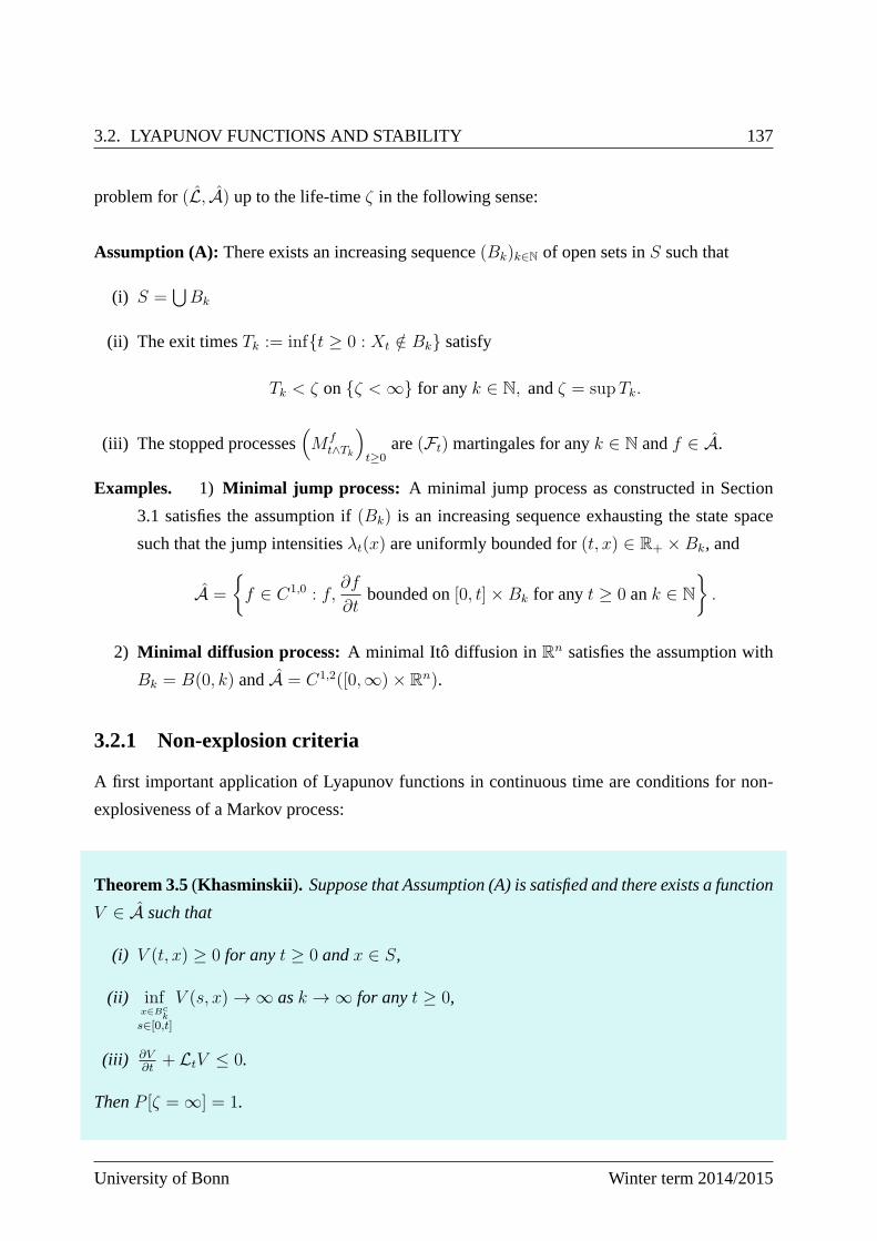
3.2. LYAPUNOV FUNCTIONS AND STABILITY 137
problem for(L, A) up to the life-timeζ in the following sense:
Assumption (A): There exists an increasing sequence(Bk)k∈N of open sets inS such that
(i) S =⋃Bk
(ii) The exit timesTk := inft ≥ 0 : Xt /∈ Bk satisfy
Tk < ζ onζ <∞ for anyk ∈ N, andζ = supTk.
(iii) The stopped processes(M f
t∧Tk
)t≥0
are(Ft) martingales for anyk ∈ N andf ∈ A.
Examples. 1) Minimal jump process: A minimal jump process as constructed in Section
3.1 satisfies the assumption if(Bk) is an increasing sequence exhausting the state space
such that the jump intensitiesλt(x) are uniformly bounded for(t, x) ∈ R+ × Bk, and
A =
f ∈ C1,0 : f,
∂f
∂tbounded on[0, t]×Bk for anyt ≥ 0 ank ∈ N
.
2) Minimal diffusion process: A minimal Itô diffusion inRn satisfies the assumption with
Bk = B(0, k) andA = C1,2([0,∞)× Rn).
3.2.1 Non-explosion criteria
A first important application of Lyapunov functions in continuous time are conditions for non-
explosiveness of a Markov process:
Theorem 3.5(Khasminskii). Suppose that Assumption (A) is satisfied and there exists a function
V ∈ A such that
(i) V (t, x) ≥ 0 for anyt ≥ 0 andx ∈ S,
(ii) infx∈Bc
ks∈[0,t]
V (s, x) → ∞ ask → ∞ for anyt ≥ 0,
(iii) ∂V∂t
+ LtV ≤ 0.
ThenP [ζ = ∞] = 1.
University of Bonn Winter term 2014/2015
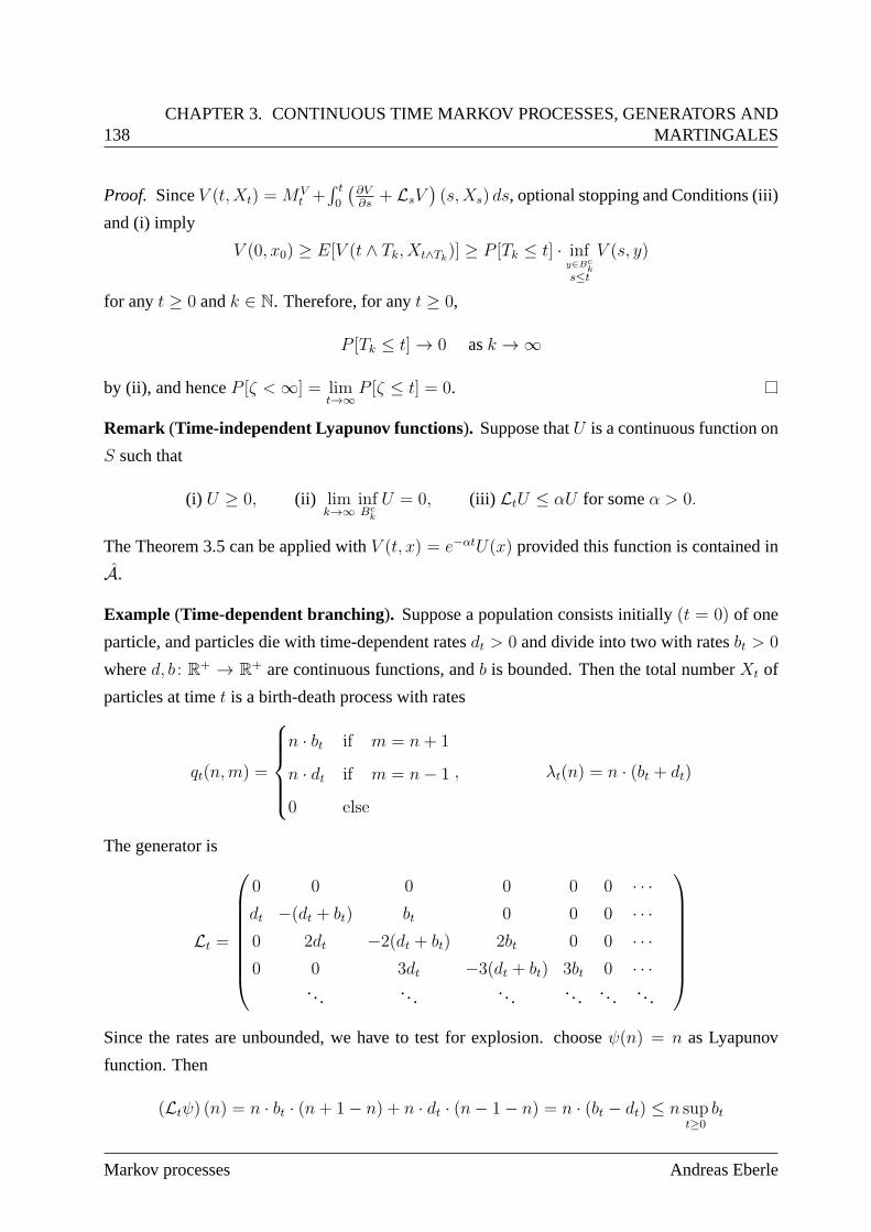
138CHAPTER 3. CONTINUOUS TIME MARKOV PROCESSES, GENERATORS AND
MARTINGALES
Proof. SinceV (t,Xt) =MVt +´ t
0
(∂V∂s
+ LsV)(s,Xs) ds, optional stopping and Conditions (iii)
and (i) imply
V (0, x0) ≥ E[V (t ∧ Tk, Xt∧Tk)] ≥ P [Tk ≤ t] · inf
y∈Bck
s≤t
V (s, y)
for anyt ≥ 0 andk ∈ N. Therefore, for anyt ≥ 0,
P [Tk ≤ t] → 0 ask → ∞
by (ii), and henceP [ζ <∞] = limt→∞
P [ζ ≤ t] = 0.
Remark (Time-independent Lyapunov functions). Suppose thatU is a continuous function on
S such that
(i) U ≥ 0, (ii) limk→∞
infBc
k
U = 0, (iii) LtU ≤ αU for someα > 0.
The Theorem 3.5 can be applied withV (t, x) = e−αtU(x) provided this function is contained in
A.
Example (Time-dependent branching). Suppose a population consists initially(t = 0) of one
particle, and particles die with time-dependent ratesdt > 0 and divide into two with ratesbt > 0
whered, b : R+ → R+ are continuous functions, andb is bounded. Then the total numberXt of
particles at timet is a birth-death process with rates
qt(n,m) =
n · bt if m = n+ 1
n · dt if m = n− 1
0 else
, λt(n) = n · (bt + dt)
The generator is
Lt =
0 0 0 0 0 0 · · ·dt −(dt + bt) bt 0 0 0 · · ·0 2dt −2(dt + bt) 2bt 0 0 · · ·0 0 3dt −3(dt + bt) 3bt 0 · · ·
. .. . . . . . . .. . . . . . . .
Since the rates are unbounded, we have to test for explosion.chooseψ(n) = n as Lyapunov
function. Then
(Ltψ) (n) = n · bt · (n+ 1− n) + n · dt · (n− 1− n) = n · (bt − dt) ≤ n supt≥0
bt
Markov processes Andreas Eberle
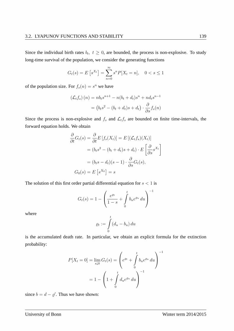
3.2. LYAPUNOV FUNCTIONS AND STABILITY 139
Since the individual birth ratesbt, t ≥ 0, are bounded, the process is non-explosive. To study
long-time survival of the population, we consider the generating functions
Gt(s) = E[sXt]=
∞∑
n=0
snP [Xt = n], 0 < s ≤ 1
of the population size. Forfs(n) = sn we have
(Ltfs) (n) = nbtsn+1 − n(bt + dt)s
n + ndtsn−1
=(bts
2 − (bt + dt)s+ dt)· ∂∂sfs(n)
Since the process is non-explosive andfs andLtfs are bounded on finite time-intervals, the
forward equation holds. We obtain
∂
∂tGt(s) =
∂
∂tE [fs(Xt)] = E [(Ltfs)(Xt)]
= (bts2 − (bt + dt)s+ dt) · E
[∂
∂ssXt
]
= (bts− dt)(s− 1) · ∂∂sGt(s),
G0(s) = E[sX0]= s
The solution of this first order partial differential equation fors < 1 is
Gt(s) = 1−
et
1− s+
tˆ
0
bneu du
−1
where
t :=
tˆ
0
(du − bu) du
is the accumulated death rate. In particular, we obtain an explicit formula for the extinction
probability:
P [Xt = 0] = lims↓0
Gt(s) =
et +
tˆ
0
bneu du
−1
= 1−
1 +
tˆ
0
dueu du
−1
sinceb = d− ′. Thus we have shown:
University of Bonn Winter term 2014/2015
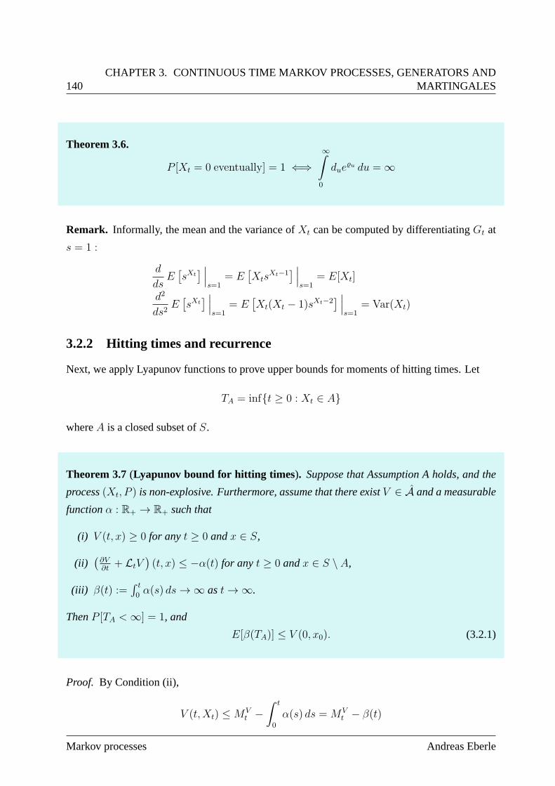
140CHAPTER 3. CONTINUOUS TIME MARKOV PROCESSES, GENERATORS AND
MARTINGALES
Theorem 3.6.
P [Xt = 0 eventually] = 1 ⇐⇒∞
0
dueu du = ∞
Remark. Informally, the mean and the variance ofXt can be computed by differentiatingGt at
s = 1 :
d
dsE[sXt] ∣∣∣
s=1= E
[Xts
Xt−1] ∣∣∣
s=1= E[Xt]
d2
ds2E[sXt] ∣∣∣
s=1= E
[Xt(Xt − 1)sXt−2
] ∣∣∣s=1
= Var(Xt)
3.2.2 Hitting times and recurrence
Next, we apply Lyapunov functions to prove upper bounds for moments of hitting times. Let
TA = inft ≥ 0 : Xt ∈ A
whereA is a closed subset ofS.
Theorem 3.7(Lyapunov bound for hitting times ). Suppose that Assumption A holds, and the
process(Xt, P ) is non-explosive. Furthermore, assume that there existV ∈ A and a measurable
functionα : R+ → R+ such that
(i) V (t, x) ≥ 0 for anyt ≥ 0 andx ∈ S,
(ii)(∂V∂t
+ LtV)(t, x) ≤ −α(t) for anyt ≥ 0 andx ∈ S \ A,
(iii) β(t) :=´ t
0α(s) ds→ ∞ ast→ ∞.
ThenP [TA <∞] = 1, and
E[β(TA)] ≤ V (0, x0). (3.2.1)
Proof. By Condition (ii),
V (t,Xt) ≤MVt −ˆ t
0
α(s) ds =MVt − β(t)
Markov processes Andreas Eberle
3.2. LYAPUNOV FUNCTIONS AND STABILITY 141
holds fort < TA. For anyk ∈ N,MVt∧Tk
is a martingale. Hence by (i),
0 ≤ E [V (t ∧ TA ∧ Tk, Xt∧TA∧Tk)] ≤ V (0, x0)− E[β(t ∧ TA ∧ Tk)].
As k → ∞, Tk → ∞ almost surely, and we obtain
β(t)P [t ≤ TA] ≤ E[β(t ∧ TA)] ≤ V (0, x0)
for anyt > 0. The assertion follows ast→ ∞.
Example (Moments of hitting times).
If α(s) = csn−1 for somec > 0 andn ∈ N thenβ(s) = cnsn. In this case, (3.2.1) is the moment
bound
E[T nA] ≤
n
cV (0, x0).
3.2.3 Occupation times and existence of stationary distributions
Similarly to the discrete time case, Lyapunov conditions can also be used in continuous time to
show the existence of stationary distributions. The following exercise covers the case of diffu-
sions inRn:
Exercise (Explosion, occupation times and stationary distributions for diffusions on Rn).
Consider a diffusion process(Xt, Px) onRn solving the local martingale problem for the gener-
ator
Ltf =1
2
n∑
i,j=1
ai,j(t, x)∂2f
∂xi ∂xj+
n∑
i=1
bi(t, x)∂f
∂xi, f ∈ C1,2(R+ × Rn).
We assume that the coefficients are continuous functions andPx[X0 = x] = 1.
a) Prove that the process is non-explosive if there exist finite constantsc1, c2, r such that
tr a(t, x) ≤ c1 |x|2 and x · b(t, x) ≤ c2 |x|2 for |x| ≥ r.
b) Now suppose thatζ = ∞ almost surely, and that there existV ∈ C1,2(R+ × Rn) and
ε, c ∈ R+ such thatV ≥ 0 and
∂V
∂t+ LtV ≤ ε+ c1B onR+ × Rn,
whereB is a ball inRn. Prove that
E
[1
t
ˆ t
0
1B(Xs) ds
]≥ ε
c− V (0, x0)
ct.
University of Bonn Winter term 2014/2015
142CHAPTER 3. CONTINUOUS TIME MARKOV PROCESSES, GENERATORS AND
MARTINGALES
b) Conclude that if(Xt, Px) is a time-homogeneous Markov process and the conditions above
hold then there exists a stationary distribution.
Again the results carry over with similar proofs to general Markov processes. Let
At(B) =1
t
ˆ t
0
1B(Xs) ds
denote the relative amount of time spent by the process in thesetB during the time interval[0, t].
Lemma 3.8(Lyapunov bound for occupation times). Suppose Assumption A holds, the process
is almost surely non-explosive, and there exist constantsε, c ∈ R+ and a non-negative function
V ∈ A such that∂V
∂t+ LtV ≤ −ε+ c1B onR+ × S.
Then
E[At(B)] ≥ ε
c− V (0, x0)
ct.
Now assume that(Xt, P ) is a time-homogeneousMarkov process with transition semigroup
(pt)t≥0, and, correspondingly,Lt does not depend ont. Then by Fubini’s Theorem,
E[At(B)] =1
t
ˆ t
0
ps(x0, B) ds =: pt(x0, B).
Theorem 3.9(Existence of stationary distributions). Suppose that the assumptions in Lemma
3.8 hold, and moreover, assume thatS is σ-compact,V (t, x) = U(x) for some continuous func-
tionU : S → [0,∞), and there existε, c ∈ R+ and a compact setK ⊆ S such that
LU ≤ −ε+ c1K .
Then there exists a stationary distributionµ of (pt)t≥0.
Proof. The assumptions imply
lim inft→∞
pt(x0, K) > 0.
The assertion now follows similarly as in discrete time, cf.Theorem??.
Markov processes Andreas Eberle
3.3. SEMIGROUPS, GENERATORS AND RESOLVENTS 143
3.3 Semigroups, generators and resolvents
In the discrete time case, there is a one-to-one correspondence between generatorsL = p − I,
transition semigroupspt = pt, and time-homogeneous canonical Markov chains((Xn)n∈Z+ , (Px)x∈S)
solving the martingale problem forL on bounded measurable functions. Our goal in this section
is to establish a counterpart to the correspondence betweengenerators and transition semigroups
in continuous time. Since the generator will usually be an unbounded operator, this requires the
realization of the transition semigroup and the generator on an appropriate Banach space con-
sisting of measurable functions (or equivalence classes offunctions) on the state space(S,B).Unfortunately, there is no Banach space that is adequate for all purposes - so the realization on
a Banach space also leads to a partially more restrictive setting. Supplementary reference: for
this section are Yosida: Functional Analysis [39], Pazy: Semigroups of Linear Operators [24],
Davies: One-parameter semigroups [5] and Ethier/Kurtz [11].
We assume that we are given a time-homogeneous transition function(pt)t≥0 on (S,B), i.e.,
(i) pt(x, dy) is a sub-probability kernel on(S,B) for anyt ≥ 0, and
(ii) p0(x, ·) = δx andptps = pt+s for anyt, s ≥ 0 andx ∈ S.
Remark (Inclusion of time-inhomogeneous case). Although we restrict ourselves to the time-
homogeneous case, the time-inhomogeneous case is includedimplicitly. Indeed, if((Xt)t≥s, P(s,x))
is a time-inhomogeneous Markov process with transition function ps,t(x,B) = P(s,x)[Xt ∈ B]
then the time-space processXt = (t + s,Xt+s) is a time-homogeneous Markov process w.r.t.
P(s,x) withs state spaceR+ × S and transition function
Pt ((s, x), dudy) = δt+s(du)ps,t+s(x, dy).
3.3.1 Sub-Markovian semigroups and resolvents
The transition kernelspt act as linear operatorsf 7→ ptf on bounded measurable functions onS.
They also act onLp spaces w.r.t. a measureµ if µ is sub-invariant for the transition kernels:
Definition. A positive measureµ ∈M+(S) is calledsub-invariantw.r.t. the transition semigroup
(pt) iff µpt ≤ µ for anyt ≥ 0 in the sense thatˆ
ptfdµ ≤ˆ
fdµ for anyf ∈ F+(S) andt ≥ 0.
University of Bonn Winter term 2014/2015
144CHAPTER 3. CONTINUOUS TIME MARKOV PROCESSES, GENERATORS AND
MARTINGALES
For processes with finite life-time, non-trivial invariantmeasures often do not exist, but in many
cases non-trivial sub-invariant measures do exist.
Lemma 3.10(Sub-Markov semigroup and contraction properties). 1) Any transition func-
tion (pt)t≥0 induces asub-Markovian semigrouponFb(S) or F+(S) respectively, i.e., for
anys, t ≥ 0
(i) Semigroup property:pspt = ps+t,
(ii) Positivity preserving:f ≥ 0 ⇒ ptf ≥ 0,
(iii) pt1 ≤ 1.
2) The semigroup is contractive w.r.t. the supremum norm:
‖ptf‖sup≤ ‖f‖sup for anyt ≥ 0 andf ∈ Fb(S).
3) If µ ∈ M+(S) is a sub-invariant measure then(pt) is also contractive w.r.t. theLp(µ)
norm for everyp ∈ [1,∞]:ˆ
|ptf |pdµ ≤ˆ
|f |pdµ for anyf ∈ Lp(S, µ).
In particular, the mapf 7→ ptf respectsµ-classes.
Proof. Most of the statements are straightforward to prove and leftas an exercise. We only prove
the last statement forp ∈ [1,∞):
For t ≥ 0, the sub-Markov property impliesptf ≤ pt|f | and−ptf ≤ pt|f | for anyf ∈ Lp(S, µ).
Hence
|ptf |p ≤ (pt|f |)p ≤ pt|f |p
by Jensen’s inequality. Integration w.r.t.µ yieldsˆ
|ptf |pdµ ≤ˆ
pt|f |pdµ ≤ˆ
|f |pdµ
by the sub-invariance ofµ. Hencept is a contraction onLp(S, µ). In particular,pt respects
µ-classes sincef = g µ-a.e. ⇒ f − g = 0 µ-a.e. ⇒ pt(f − g) = 0 µ-a.e. ⇒ ptf = ptg
µ-a.e.
The theorem shows that(pt) induces contraction semigroups of linear operatorsPt on the follow-
ing Banach spaces:
• Fb(S) endowed with the supremum norm,
Markov processes Andreas Eberle
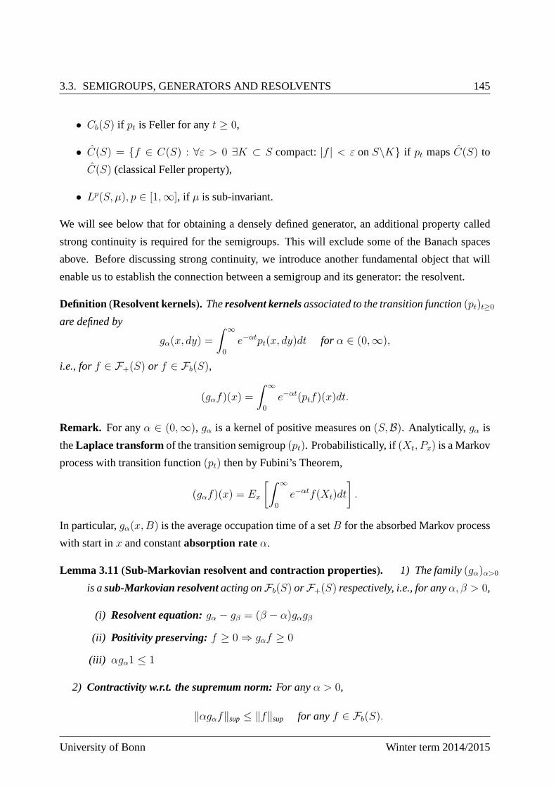
3.3. SEMIGROUPS, GENERATORS AND RESOLVENTS 145
• Cb(S) if pt is Feller for anyt ≥ 0,
• C(S) = f ∈ C(S) : ∀ε > 0 ∃K ⊂ S compact:|f | < ε onS\K if pt mapsC(S) to
C(S) (classical Feller property),
• Lp(S, µ), p ∈ [1,∞], if µ is sub-invariant.
We will see below that for obtaining a densely defined generator, an additional property called
strong continuity is required for the semigroups. This willexclude some of the Banach spaces
above. Before discussing strong continuity, we introduce another fundamental object that will
enable us to establish the connection between a semigroup and its generator: the resolvent.
Definition (Resolvent kernels). Theresolvent kernelsassociated to the transition function(pt)t≥0
are defined by
gα(x, dy) =
ˆ ∞
0
e−αtpt(x, dy)dt for α ∈ (0,∞),
i.e., forf ∈ F+(S) or f ∈ Fb(S),
(gαf)(x) =
ˆ ∞
0
e−αt(ptf)(x)dt.
Remark. For anyα ∈ (0,∞), gα is a kernel of positive measures on(S,B). Analytically, gα is
theLaplace transform of the transition semigroup(pt). Probabilistically, if(Xt, Px) is a Markov
process with transition function(pt) then by Fubini’s Theorem,
(gαf)(x) = Ex
[ˆ ∞
0
e−αtf(Xt)dt
].
In particular,gα(x,B) is the average occupation time of a setB for the absorbed Markov process
with start inx and constantabsorption rate α.
Lemma 3.11(Sub-Markovian resolvent and contraction properties). 1) The family(gα)α>0
is asub-Markovian resolventacting onFb(S) or F+(S) respectively, i.e., for anyα, β > 0,
(i) Resolvent equation:gα − gβ = (β − α)gαgβ
(ii) Positivity preserving:f ≥ 0 ⇒ gαf ≥ 0
(iii) αgα1 ≤ 1
2) Contractivity w.r.t. the supremum norm:For anyα > 0,
‖αgαf‖sup≤ ‖f‖sup for anyf ∈ Fb(S).
University of Bonn Winter term 2014/2015
146CHAPTER 3. CONTINUOUS TIME MARKOV PROCESSES, GENERATORS AND
MARTINGALES
3) Contractivity w.r.t.Lp norms: If µ ∈ M+(S) is sub-invariant w.r.t.(pt) then
‖αgαf‖Lp(S,µ) ≤ ‖f‖Lp(S,µ) for anyα > 0, p ∈ [1,∞], andf ∈ Lp(S, µ).
Proof. 1) By Fubini’s Theorem and the semigroup property,
gαgβf =
ˆ ∞
0
ˆ ∞
0
e−αte−βspt+sf ds dt
=
ˆ ∞
0
ˆ u
0
e(β−α)tdt e−βupuf du
=1
β − α(gαf − gβf)
for anyα, β > 0 andf ∈ Fb(S). This proves (i). (ii) and (iii) follow easily from the
corresponding properties for the semigroup(pt).
2),3) Let‖ · ‖ be either the supremum norm or anLp norm. Then contractivity of(pt)t≥0 w.r.t.
‖ · ‖ implies that also(αgα) is contractive w.r.t.‖ · ‖:
‖αgαf‖ ≤ˆ ∞
0
αe−αt‖ptf‖dt ≤ˆ ∞
0
αe−αtdt ‖f‖ = ‖f‖ for anyα > 0.
The lemma shows that(gα)α>0 induces contraction resolvents of linear operators(Gα)α>0 on the
Banach spacesFb(S), Cb(S) if the semigroup(pt) is Feller,C(S) if (pt) is Feller in the classical
sense, andLp(S, µ) if µ is sub-invariant for(pt). Furthermore, the resolvent equation implies that
the range of the operatorsGα is independent ofα:
(R) Range(Gα) = Range(Gβ) for anyα, β ∈ (0,∞).
This property will be important below.
3.3.2 Strong continuity and Generator
We now assume that(Pt)t≥0 is a semigroup of linear contractions on a Banach spaceE. Our
goal is to define the infinitesimal generatorL of (Pt) by Lf = limt↓0
1t(Ptf − f) for a classD of
elementsf ∈ E that forms a dense linear subspace ofE. Obviously, this can only be possible if
limt↓0
‖Ptf −f‖ = 0 for anyf ∈ D, and hence, by contractivity of the operatorsPt, for anyf ∈ E.
A semigroup with this property is called strongly continuous:
Markov processes Andreas Eberle
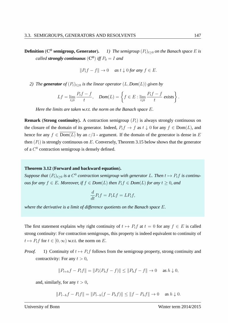
3.3. SEMIGROUPS, GENERATORS AND RESOLVENTS 147
Definition (C0 semigroup, Generator). 1) The semigroup(Pt)t≥0 on the Banach spaceE is
calledstrongly continuous(C0) iff P0 = I and
‖Ptf − f‖ → 0 ast ↓ 0 for anyf ∈ E.
2) Thegeneratorof (Pt)t≥0 is the linear operator(L,Dom(L)) given by
Lf = limt↓0
Ptf − f
t, Dom(L) =
f ∈ E : lim
t↓0
Ptf − f
texists
.
Here the limits are taken w.r.t. the norm on the Banach spaceE.
Remark (Strong continuity). A contraction semigroup(Pt) is always strongly continuous on
the closure of the domain of its generator. Indeed,Ptf → f ast ↓ 0 for anyf ∈ Dom(L), and
hence for anyf ∈ Dom(L) by anε/3 - argument. If the domain of the generator is dense inE
then(Pt) is strongly continuous onE. Conversely, Theorem 3.15 below shows that the generator
of aC0 contraction semigroup is densely defined.
Theorem 3.12(Forward and backward equation).
Suppose that(Pt)t≥0 is aC0 contraction semigroup with generatorL. Thent 7→ Ptf is continu-
ous for anyf ∈ E. Moreover, iff ∈ Dom(L) thenPtf ∈ Dom(L) for anyt ≥ 0, and
d
dtPtf = PtLf = LPtf,
where the derivative is a limit of difference quotients on theBanach spaceE.
The first statement explains why right continuity oft 7→ Ptf at t = 0 for anyf ∈ E is called
strong continuity: For contraction semigroups, this property is indeed equivalent to continuity of
t 7→ Ptf for t ∈ [0,∞) w.r.t. the norm onE.
Proof. 1) Continuity oft 7→ Ptf follows from the semigroup property, strong continuity and
contractivity: For anyt > 0,
‖Pt+hf − Ptf‖ = ‖Pt(Phf − f)‖ ≤ ‖Phf − f‖ → 0 ash ↓ 0,
and, similarly, for anyt > 0,
‖Pt−hf − Ptf‖ = ‖Pt−h(f − Phf)‖ ≤ ‖f − Phf‖ → 0 ash ↓ 0.
University of Bonn Winter term 2014/2015
148CHAPTER 3. CONTINUOUS TIME MARKOV PROCESSES, GENERATORS AND
MARTINGALES
2) Similarly, the forward equationddtPtf = PtLf follows from the semigroup property, con-
tractivity, strong continuity and the definition of the generator: For anyf ∈ Dom(L) and
t ≥ 0,1
h(Pt+hf − Ptf) = Pt
Phf − f
h→ PtLf ash ↓ 0,
and, fort > 0,
1
−h(Pt−hf − Ptf) = Pt−hPhf − f
h→ PtLf ash ↓ 0
by strong continuity.
3) Finally, the backward equationddtPtf = LPtf is a consequence of the forward equation:
Forf ∈ Dom(L) andt ≥ 0,
PhPtf − Ptf
h=
1
h(Pt+hf − Ptf) → PtLf ash ↓ 0.
HencePtf is in the domain of the generator, andLPtf = PtLf = ddtPtf .
3.3.3 Strong continuity of transition semigroups of Markov processes
Let us now assume again that(pt)t≥0 is the transition function of aright-continuoustime homo-
geneous Markov process((Xt)t≥0, (Px)x∈S) defined for any initial valuex ∈ S. We have shown
above that(pt) induces contraction semigroups on different Banach spaces consisting of func-
tions (or equivalence classes of functions) fromS to R. The following example shows, however,
that these semigroups are not necessarily strongly continuous:
Example (Strong continuity of the heat semigroup). Let S = R1. The heat semigroup(pt) is
the transition semigroup of Brownian motion onS. It is given explicitly by
(ptf)(x) = (f ∗ ϕt)(x) =
ˆ
R
f(y)ϕt(x− y) dy,
whereϕt(z) = (2πt)−1/2 exp (−z2/(2t)) is the density of the normal distributionN(0, t). The
heat semigroup induces contraction semigroups on the BanachspacesFb(R), Cb(R), C(R) and
Lp(R, dx) for p ∈ [1,∞]. However, the semigroups onFb(R), Cb(R) andL∞(R, dx) are not
strongly continuous. Indeed, sinceptf is a continuous function for anyf ∈ Fb(R),
‖pt1(0,1) − 1(0,1)‖∞ ≥ 1
2for anyt > 0.
Markov processes Andreas Eberle
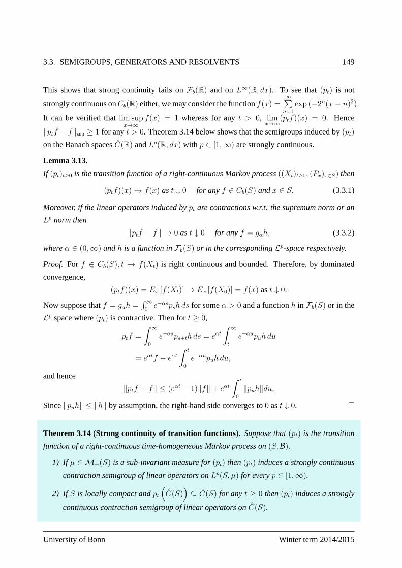
3.3. SEMIGROUPS, GENERATORS AND RESOLVENTS 149
This shows that strong continuity fails onFb(R) and onL∞(R, dx). To see that(pt) is not
strongly continuous onCb(R) either, we may consider the functionf(x) =∞∑n=1
exp (−2n(x− n)2).
It can be verified thatlim supx→∞
f(x) = 1 whereas for anyt > 0, limx→∞
(ptf)(x) = 0. Hence
‖ptf − f‖sup≥ 1 for anyt > 0. Theorem 3.14 below shows that the semigroups induced by(pt)
on the Banach spacesC(R) andLp(R, dx) with p ∈ [1,∞) are strongly continuous.
Lemma 3.13.
If (pt)t≥0 is the transition function of a right-continuous Markov process((Xt)t≥0, (Px)x∈S) then
(ptf)(x) → f(x) ast ↓ 0 for anyf ∈ Cb(S) andx ∈ S. (3.3.1)
Moreover, if the linear operators induced bypt are contractions w.r.t. the supremum norm or an
Lp norm then
‖ptf − f‖ → 0 ast ↓ 0 for anyf = gαh, (3.3.2)
whereα ∈ (0,∞) andh is a function inFb(S) or in the correspondingLp-space respectively.
Proof. For f ∈ Cb(S), t 7→ f(Xt) is right continuous and bounded. Therefore, by dominated
convergence,
(ptf)(x) = Ex [f(Xt)] → Ex [f(X0)] = f(x) ast ↓ 0.
Now suppose thatf = gαh =´∞0e−αspsh ds for someα > 0 and a functionh in Fb(S) or in the
Lp space where(pt) is contractive. Then fort ≥ 0,
ptf =
ˆ ∞
0
e−αsps+th ds = eαtˆ ∞
t
e−αupuh du
= eαtf − eαtˆ t
0
e−αupuh du,
and hence
‖ptf − f‖ ≤ (eαt − 1)‖f‖+ eαtˆ t
0
‖puh‖du.
Since‖puh‖ ≤ ‖h‖ by assumption, the right-hand side converges to0 ast ↓ 0.
Theorem 3.14(Strong continuity of transition functions ). Suppose that(pt) is the transition
function of a right-continuous time-homogeneous Markov process on(S,B).
1) If µ ∈ M+(S) is a sub-invariant measure for(pt) then(pt) induces a strongly continuous
contraction semigroup of linear operators onLp(S, µ) for everyp ∈ [1,∞).
2) If S is locally compact andpt(C(S)
)⊆ C(S) for anyt ≥ 0 then(pt) induces a strongly
continuous contraction semigroup of linear operators onC(S).
University of Bonn Winter term 2014/2015
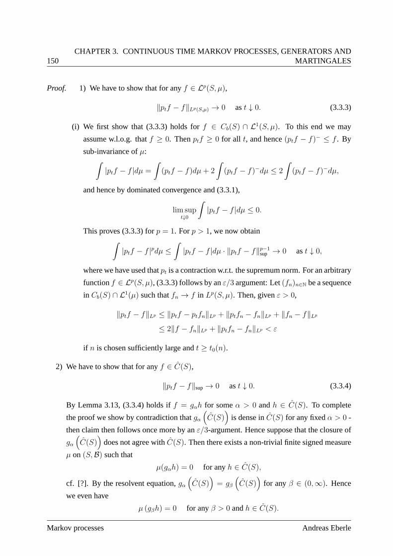
150CHAPTER 3. CONTINUOUS TIME MARKOV PROCESSES, GENERATORS AND
MARTINGALES
Proof. 1) We have to show that for anyf ∈ Lp(S, µ),
‖ptf − f‖Lp(S,µ) → 0 ast ↓ 0. (3.3.3)
(i) We first show that (3.3.3) holds forf ∈ Cb(S) ∩ L1(S, µ). To this end we may
assume w.l.o.g. thatf ≥ 0. Thenptf ≥ 0 for all t, and hence(ptf − f)− ≤ f . By
sub-invariance ofµ:ˆ
|ptf − f |dµ =
ˆ
(ptf − f)dµ+ 2
ˆ
(ptf − f)−dµ ≤ 2
ˆ
(ptf − f)−dµ,
and hence by dominated convergence and (3.3.1),
lim supt↓0
ˆ
|ptf − f |dµ ≤ 0.
This proves (3.3.3) forp = 1. Forp > 1, we now obtainˆ
|ptf − f |pdµ ≤ˆ
|ptf − f |dµ · ‖ptf − f‖p−1sup → 0 ast ↓ 0,
where we have used thatpt is a contraction w.r.t. the supremum norm. For an arbitrary
functionf ∈ Lp(S, µ), (3.3.3) follows by anε/3 argument: Let(fn)n∈N be a sequence
in Cb(S) ∩ L1(µ) such thatfn → f in Lp(S, µ). Then, givenε > 0,
‖ptf − f‖Lp ≤ ‖ptf − ptfn‖Lp + ‖ptfn − fn‖Lp + ‖fn − f‖Lp
≤ 2‖f − fn‖Lp + ‖ptfn − fn‖Lp < ε
if n is chosen sufficiently large andt ≥ t0(n).
2) We have to show that for anyf ∈ C(S),
‖ptf − f‖sup→ 0 ast ↓ 0. (3.3.4)
By Lemma 3.13, (3.3.4) holds iff = gαh for someα > 0 andh ∈ C(S). To complete
the proof we show by contradiction thatgα(C(S)
)is dense inC(S) for any fixedα > 0 -
then claim then follows once more by anε/3-argument. Hence suppose that the closure of
gα
(C(S)
)does not agree withC(S). Then there exists a non-trivial finite signed measure
µ on (S,B) such that
µ(gαh) = 0 for anyh ∈ C(S),
cf. [?]. By the resolvent equation,gα(C(S)
)= gβ
(C(S)
)for anyβ ∈ (0,∞). Hence
we even have
µ (gβh) = 0 for anyβ > 0 andh ∈ C(S).
Markov processes Andreas Eberle
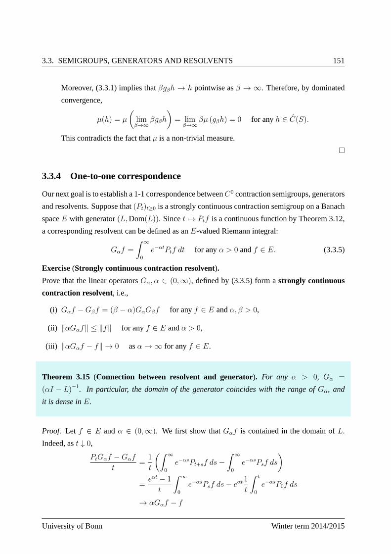
3.3. SEMIGROUPS, GENERATORS AND RESOLVENTS 151
Moreover, (3.3.1) implies thatβgβh → h pointwise asβ → ∞. Therefore, by dominated
convergence,
µ(h) = µ
(limβ→∞
βgβh
)= lim
β→∞βµ (gβh) = 0 for anyh ∈ C(S).
This contradicts the fact thatµ is a non-trivial measure.
3.3.4 One-to-one correspondence
Our next goal is to establish a 1-1 correspondence betweenC0 contraction semigroups, generators
and resolvents. Suppose that(Pt)t≥0 is a strongly continuous contraction semigroup on a Banach
spaceE with generator(L,Dom(L)). Sincet 7→ Ptf is a continuous function by Theorem 3.12,
a corresponding resolvent can be defined as anE-valued Riemann integral:
Gαf =
ˆ ∞
0
e−αtPtf dt for anyα > 0 andf ∈ E. (3.3.5)
Exercise(Strongly continuous contraction resolvent).
Prove that the linear operatorsGα, α ∈ (0,∞), defined by (3.3.5) form astrongly continuous
contraction resolvent, i.e.,
(i) Gαf −Gβf = (β − α)GαGβf for anyf ∈ E andα, β > 0,
(ii) ‖αGαf‖ ≤ ‖f‖ for anyf ∈ E andα > 0,
(iii) ‖αGαf − f‖ → 0 asα → ∞ for anyf ∈ E.
Theorem 3.15 (Connection between resolvent and generator). For any α > 0, Gα =
(αI − L)−1. In particular, the domain of the generator coincides with the range ofGα, and
it is dense inE.
Proof. Let f ∈ E andα ∈ (0,∞). We first show thatGαf is contained in the domain ofL.
Indeed, ast ↓ 0,
PtGαf −Gαf
t=
1
t
(ˆ ∞
0
e−αsPt+sf ds−ˆ ∞
0
e−αsPsf ds
)
=eαt − 1
t
ˆ ∞
0
e−αsPsf ds− eαt1
t
ˆ t
0
e−αsP0f ds
→ αGαf − f
University of Bonn Winter term 2014/2015
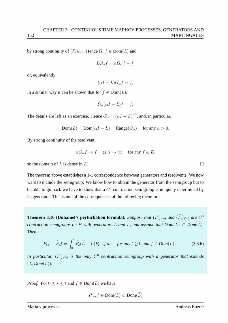
152CHAPTER 3. CONTINUOUS TIME MARKOV PROCESSES, GENERATORS AND
MARTINGALES
by strong continuity of(Pt)t≥0. HenceGαf ∈ Dom(L) and
LGαf = αGαf − f,
or, equivalently
(αI − L)Gαf = f.
In a similar way it can be shown that forf ∈ Dom(L),
Gα(αI − L)f = f.
The details are left as an exercise. HenceGα = (αI − L)−1, and, in particular,
Dom(L) = Dom(αI − L) = Range(Gα) for anyα > 0.
By strong continuity of the resolvent,
αGαf → f asα → ∞ for anyf ∈ E,
so the domain ofL is dense inE.
The theorem above establishes a 1-1 correspondence betweengenerators and resolvents. We now
want to include the semigroup: We know how to obtain the generator from the semigroup but to
be able to go back we have to show that aC0 contraction semigroup is uniquely determined by
its generator. This is one of the consequences of the following theorem:
Theorem 3.16(Duhamel’s perturbation formula ). Suppose that(Pt)t≥0 and (Pt)t≥0 are C0
contraction semigroups onE with generatorsL and L, and assume that Dom(L) ⊂ Dom(L).
Then
Ptf − Ptf =
ˆ t
0
Ps(L− L)Pt−sf ds for anyt ≥ 0 andf ∈ Dom(L). (3.3.6)
In particular, (Pt)t≥0 is the onlyC0 contraction semigroup with a generator that extends
(L,Dom(L)).
Proof. For0 ≤ s ≤ t andf ∈ Dom(L) we have
Pt−sf ∈ Dom(L) ⊂ Dom(L)
Markov processes Andreas Eberle
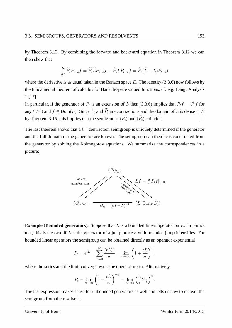
3.3. SEMIGROUPS, GENERATORS AND RESOLVENTS 153
by Theorem 3.12. By combining the forward and backward equation in Theorem 3.12 we can
then show that
d
dsPsPt−sf = PsLPt−sf − PsLPt−sf = Ps(L− L)Pt−sf
where the derivative is as usual taken in the Banach spaceE. The identity (3.3.6) now follows by
the fundamental theorem of calculus for Banach-space valuedfunctions, cf. e.g. Lang: Analysis
1 [17].
In particular, if the generator ofPt is an extension ofL then (3.3.6) implies thatPtf = Ptf for
anyt ≥ 0 andf ∈ Dom(L). SincePt andPt are contractions and the domain ofL is dense inE
by Theorem 3.15, this implies that the semigroups(Pt) and(Pt) coincide.
The last theorem shows that aC0 contraction semigroup is uniquely determined if the generator
and the full domain of the generator are known. The semigroupcan then be reconstructed from
the generator by solving the Kolmogorov equations. We summarize the correspondences in a
picture:
(Gα)α>0
(Pt)t≥0
(L,Dom(L))
Laplace
transformation
Gα = (αI − L)−1
Lf = ddtPtf |t=0+Kolmogorov
equations
Example (Bounded generators). Suppose thatL is a bounded linear operator onE. In partic-
ular, this is the case ifL is the generator of a jump process with bounded jump intensities. For
bounded linear operators the semigroup can be obtained directly as an operator exponential
Pt = etL =∞∑
n=0
(tL)n
n!= lim
n→∞
(1 +
tL
n
)n
,
where the series and the limit converge w.r.t. the operator norm. Alternatively,
Pt = limn→∞
(1− tL
n
)−n
= limn→∞
(ntGn
t
)n.
The last expression makes sense for unbounded generators aswell and tells us how to recover the
semigroup from the resolvent.
University of Bonn Winter term 2014/2015
154CHAPTER 3. CONTINUOUS TIME MARKOV PROCESSES, GENERATORS AND
MARTINGALES
3.3.5 Hille-Yosida-Theorem
We conclude this section with an important theoretical result showing which linear operators are
generators ofC0 contraction semigroups. The proof will be sketched, cf. e.g. Ethier & Kurtz
[11] for a detailed proof.
Theorem 3.17(Hille-Yosida). A linear operator(L,Dom(L)) on the Banach spaceE is the
generator of a strongly continuous contraction semigroup if and only if the following conditions
hold
(i) Dom(L) is dense inE,
(ii) Range(αI − L) = E for someα > 0 (or, equivalently, for anyα > 0),
(iii) L is dissipative, i.e.,
‖αf − Lf‖ ≥ α‖f‖ for anyα > 0, f ∈ Dom(L).
Proof. “⇒”: If L generates aC0 contraction semigroup then by Theorem 3.15,(αI−L)−1 = Gα
where(Gα) is the correspondingC0 contraction resolvent. In particular, the domain ofL is the
range ofGα, and the range ofαI −L is the domain ofGα. This shows that properties (i) and (ii)
hold. Furthermore, anyf ∈ Dom(L) can be represented asf = Gαg for someg ∈ E. Hence
α‖f‖ = ‖αGαg‖ ≤ ‖g‖ = ‖αf − Lf‖
by contractivity ofαGα.
“⇐”: We only sketch this part of the proof. The key idea is to “regularize” the possibly un-
bounded linear operatorL via the resolvent. By properties (ii) and (iii), the operatorαI − L is
invertible for anyα > 0, and the inverseGα := (αI−L)−1 is one-to-one fromE onto the domain
of L. Furthermore, it can be shown that(Gα)α>0 is aC0 contraction resolvent. Therefore, for
anyf ∈ Dom(L),
Lf = limα→∞
αGαLf = limα→∞
L(α)f
whereL(α) is thebounded linear operator defined by
L(α) = αLGα = α2Gα − αI for α ∈ (0,∞).
Markov processes Andreas Eberle
3.4. MARTINGALE PROBLEMS FOR MARKOV PROCESSES 155
Here we have used thatL andGα commute and(αI − L)Gα = I. The approximation by the
bounded linear operatorsL(α) is called theYosida approximation of L. One verifies now that
the operator exponentials
P(α)t = etL
(α)
=∞∑
n=0
1
n!
(tL(α)
)n, t ∈ [0,∞),
form aC0 contraction semigroup with generatorL(α) for everyα > 0. Moreover, since(L(α)f
)α∈N
is a Cauchy sequence for anyf ∈Dom(L), Duhamel’s formula (3.3.6) shows that also(P
(α)t f
)α∈N
is a Cauchy sequence for anyt ≥ 0 andf ∈ Dom(L). We can hence define
Ptf = limα→∞
P(α)t f for anyt ≥ 0 andf ∈ Dom(L). (3.3.7)
SinceP (α)t is a contraction for everyt andα, Pt is a contraction, too. Since the domain ofL is
dense inE by Assumption (i), eachPt can be extended to a linear contraction onE, and (3.3.7)
extends tof ∈ E. Now it can be verified that the limiting operatorsPt form aC0 contraction
semigroup with generatorL.
Exercise(Semigroups generated by self-adjoint operators on Hilbertspaces). Show that ifE
is a Hilbert space (for example anL2 space) with norm‖f‖ = (f, f)1/2, andL is aself-adjoint
linear operator, i.e.,
(L,Dom(L)) = (L∗,Dom(L∗)),
thenL is the generator of aC0 contraction semigroup onE if and only ifL is negative definite,
i.e.,
(f, Lf) ≤ 0 for anyf ∈ Dom(L).
In this case, theC0 semigroup generated byL is given by
Pt = etL for anyt ≥ 0,
where the exponential is defined by spectral theory, cf. e.g.Reed& Simon:Methods of modern
mathematical physics I [28], II [26], III [29], IV [27].
3.4 Martingale problems for Markov processes
In the last section we have seen that there is a one-to-one correspondence between strongly
continuous contraction semigroups on Banach spaces and their generators. The connection to
Markov processes can be made via the martingale problem. We assume at first that we are given
University of Bonn Winter term 2014/2015
156CHAPTER 3. CONTINUOUS TIME MARKOV PROCESSES, GENERATORS AND
MARTINGALES
a right-continuous time-homogeneous Markov process((Xt)t∈[0,∞), (Px)x∈S)) with state space
(S,B) andtransition semigroup(pt)t≥0. Suppose moreover thatE is either a closed linear sub-
space ofFb(S) endowed with the supremum norm such that
(A1) pt(E) ⊆ E for anyt ≥ 0, and
(A2) µ, ν ∈ P(S) with´
fdµ =´
fdν∀f ∈ E ⇒ µ = ν,
orE = Lp(S, µ) for somep ∈ [1,∞) and a(pt)-sub-invariant measureµ ∈ M+(S).
3.4.1 From Martingale problem to Generator
In many situations it is known that for anyx ∈ S, the process((Xt)t≥0, Px) solves the martingale
problem for some linear operator defined on “nice” functionsonS. Hence letA ⊂ E be a dense
linear subspace of the Banach spaceE, and let
L : A ⊂ E → E
be a linear operator.
Theorem 3.18(From the martingale problem to C0 semigroups and generators). Suppose
that for anyx ∈ S andf ∈ A, the random variablesf(Xt) and (Lf)(Xt) are integrable w.r.t.
Px for anyt ≥ 0, and the process
M ft = f(Xt)−
ˆ t
0
(Lf)(Xs)ds
is an (FXt ) martingale w.r.t.Px. Then the transition function(pt)t≥0 induces a strongly contin-
uous contraction semigroup(Pt)t≥0 of linear operators onE, and the generator(L,Dom(L)) of
(Pt)t≥0 is an extension of(L,A).
Remark. In the case of Markov processes with finite life-time the statement is still valid if func-
tions f : S → R are extended trivially toS ∪ ∆ by settingf(∆) := 0. This convention is
always tacitly assumed below.
Markov processes Andreas Eberle
3.4. MARTINGALE PROBLEMS FOR MARKOV PROCESSES 157
Proof. The martingale property forM f w.r.t. Px implies that the transition function(pt) satisfies
the forward equation
(ptf)(x)− f(x) = Ex[f(Xt)− f(X0)] = Ex
[ˆ t
0
(Lf)(Xs)ds
]
=
ˆ t
0
Ex[(Lf)(Xs)]ds =
ˆ t
0
(psLf)(x)ds (3.4.1)
for anyt ≥ 0, x ∈ S andf ∈ A. By the assumptions and Lemma 3.10,pt is contractive w.r.t. the
norm onE for anyt ≥ 0. Therefore, by (3.4.1),
‖ptf − f‖E ≤ˆ t
0
‖psLf‖Eds ≤ t‖Lf‖E → 0 ast ↓ 0
for any f ∈ A. SinceA is a dense linear subspace ofE, an ε/3 argument shows that the
contraction semigroup(Pt) induced by(pt) onE is strongly continuous. Furthermore, (3.4.1)
implies that ∥∥∥∥ptf − f
t− Lf
∥∥∥∥E
≤ 1
t
ˆ t
0
‖psLf − Lf‖Eds→ 0 ast ↓ 0 (3.4.2)
for any f ∈ A. Here we have used thatlims↓0
psLf = Lf by the strong continuity. By (3.4.2),
the functions inA are contained in the domain of the generatorL of (Pt), andLf = Lf for any
f ∈ A.
3.4.2 Identification of the generator
We now assume thatL is the generator of a strongly continuous contraction semigroup (Pt)t≥0
onE, and that(L,Dom(L)) is an extension of(L,A). We have seen above that this is what can
usually be deduced from knowing that the Markov process solves the martingale problem for any
initial valuex ∈ S. The next important question is whether the generatorL and (hence) theC0
semigroup(Pt) are already uniquely determined by the fact thatL extends(L,A). In general the
answer is negative - even thoughA is a dense subspace ofE!
Example (Brownian motion with reflection and Brownian motion with absorption).
Let S = [0,∞) andE = L2(S, dx). We consider the linear operatorL = 12
d2
dx2 with dense
domainA = C∞0 (0,∞) ⊂ L2(S, dx). Suppose that((Bt)t≥0, (Px)x∈R) is a canonical Brownian
motion onR. Then we can construct several Markov processes onS which induceC0 contraction
semigroups onE with generators that extends(L,A). In particular:
• Brownian motion on R+ with reflection at 0 is defined by
Xt = |Bt| for anyt ≥ 0.
University of Bonn Winter term 2014/2015
158CHAPTER 3. CONTINUOUS TIME MARKOV PROCESSES, GENERATORS AND
MARTINGALES
• Brownian motion on R+ with absorption at 0 is defined by
Xt =
Bt for t < TB
0 ,
∆ for t ≥ TB0 ,
whereTB0 = inft ≥ 0 : Bt = 0 is the first hitting time of0 for (Bt).
Exercise. Prove that both(Xt, Px) and(Xt, Px) are right-continuous Markov processes that in-
duceC0 contraction semigroups onE = L2(R+, dx). Moreover, show that both generators
extend the operator(12
d2
dx2 , C∞0 (0,∞)). In which sense do the generators differ from each other?
The example above shows that it is not always enough to know the generator on a dense sub-
space of the corresponding Banach spaceE. Instead, what is really required for identifying the
generatorL, is to know its values on a subspace that is dense in the domainof L w.r.t. the graph
norm
‖f‖L := ‖f‖E + ‖Lf‖E.
Definition (Closability and closure of linear operators, operator cores). 1) A linear oper-
ator (L,A) is calledclosableiff it has a closed extension.
2) In this case, the smallest closed extension(L,Dom(L)) is called theclosureof (L,A). It
is given explicitly by
Dom(L) = completion ofA w.r.t. the graph norm‖ · ‖L,Lf = lim
n→∞Lfn for any sequence(fn)n∈N in A such thatfn → f in E (3.4.3)
and(Lfn)n∈N is a Cauchy sequence.
3) Suppose thatL is a linear operator onE with A ⊆ Dom(L). ThenA is called acore for
L iff A is dense in Dom(L) w.r.t. the graph norm‖ · ‖L.
It is easy to verify that if an operator is closable then the extension defined by (3.4.3) is indeed
the smallest closed extension. Since the graph norm is stronger than the norm onE, the domain
of the closure is a linear subspace ofE. The graph of the closure is exactly the closure of the
graph of the original operator inE × E. There are operators that are not closable, but in the
setup considered above we already know that there is a closedextension of(L,A) given by the
generator(L,Dom(L)). The subspaceA ⊆ Dom(L) is a core forL if and only if (L,Dom(L))
is the closure of(L,A).
Markov processes Andreas Eberle
3.4. MARTINGALE PROBLEMS FOR MARKOV PROCESSES 159
Theorem 3.19(Strong uniqueness). Suppose thatA is a dense subspace of the domain of the
generatorL. Then the following statements are equivalent:
(i) A is a core forL.
(ii) Ptf is contained in the completion ofA w.r.t. the graph norm‖ · ‖L for anyf ∈ Dom(L)
andt ∈ (0,∞).
If (i) or (ii) hold then
(iii) (Pt)t≥0 is the only strongly continuous contraction semigroup onE with a generator that
extends(L,A).
Proof. (i) ⇒ (ii) holds since by Theorem 3.12,Ptf is contained in the domain ofL for anyt > 0
andf ∈ Dom(L).
(ii) ⇒ (i): Let f ∈ Dom(L). We have to prove thatf can be approximated by functions in the
closureALof A w.r.t. the graph norm ofL. If (ii) holds this can be done by regularizingf via
the semigroup: For anyt > 0, Ptf is contained in the closure ofA w.r.t. the graph norm by (ii).
Moreover,Ptf converges tof ast ↓ 0 by strong continuity, and
LPtf = PtLf → Lf ast ↓ 0
by strong continuity and Theorem 3.12. So
‖Ptf − f‖L → 0 ast ↓ 0,
and thusf is also contained in the closure ofA w.r.t. the graph norm.
(i) ⇒ (iii): If (i) holds and (P )t≥0 is aC0 contraction semigroup with a generatorL extending
(L,A) thenL is also an extension ofL, because it is a closed operator by Theorem 3.15. Hence
the semigroups(Pt) and(Pt) agree by Theorem 3.16.
We now apply Theorem 3.19 to identify exactly the domain of the generator of Brownian motion
onRn. The transition semigroup of Brownian motion is the heat semigroup given by
(ptf)(x) = (f ∗ ϕt)(x) =
ˆ
Rn
f(y)ϕt(x− y)dy for anyt ≥ 0,
whereϕt(x) = (2πt)−n/2 exp (−|x|2/(2t)).
University of Bonn Winter term 2014/2015
160CHAPTER 3. CONTINUOUS TIME MARKOV PROCESSES, GENERATORS AND
MARTINGALES
Corollary 3.20 (Generator of Brownian motion). The transition function(pt)t≥0 of Brownian
motion induces strongly continuous contraction semigroups on C(Rn) and onLp(Rn, dx) for
everyp ∈ [1,∞). The generators of these semigroups are given by
L =1
2∆, Dom(L) = C∞
0 (Rn)∆,
whereC∞0 (Rn)
∆stands for the completion ofC∞
0 (Rn) w.r.t. the graph norm of the Laplacian
on the underlying Banach spaceC(Rn), Lp(Rn, dx) respectively. In particular, the domain ofL
contains allC2 functions with derivatives up to second order inC(Rn), Lp(Rn, dx) respectively.
Example (Generator of Brownian motion on R). In the one-dimensional case, the generators
are given explicitly by
Lf =1
2f ′′, Dom(L) =
f ∈ C(R) ∩ C2(R) : f ′′ ∈ C(R)
, (3.4.4)
Lf =1
2f ′′, Dom(L) =
f ∈ Lp(R, dx) ∩ C1(R) : f ′ absolutely continuous,f ′′ ∈ Lp(R, dx)
,
(3.4.5)
respectively.
Remark (Domain in multi-dimensional case, Sobolev spaces). In dimensionsn ≥ 2, the do-
mains of the generators contain functions that are not twicedifferentiable in the classical sense.
The domain of theLp generator is the Sobolev spaceH2,p(Rn, dx) consisting ofweaklytwice
differentiable functions with derivatives up to second order inLp(Rn, dx), cf. e.g. [XXX].
Proof. By Itô’s formula, Brownian motion(Bt, Px) solves the martingale problem for the opera-
tor 12∆ with domainC∞
0 (Rn). Moreover, Lebesgue measure is invariant for the transition kernels
pt since by Fubini’s theorem,
ˆ
Rn
ptfdx =
ˆ
Rn
ˆ
Rn
ϕt(x− y)f(y)dydx =
ˆ
Rn
f(y)dy for anyf ∈ F+(Rn).
Hence by Theorem 3.18,(pt)t≥0 inducesC0 contraction semigroups onC(S) and onLp(Rn, dx)
for p ∈ [1,∞), and the generators are extensions of(12∆, C∞
0 (Rn)). A standard approximation
argument shows that the completionsC∞0 (Rn)
∆w.r.t. the graph norms contain all functions
in C2(Rn) with derivatives up to second order inC(Rn), Lp(Rn, dx) respectively. Therefore,
ptf = f ∗ ϕt is contained inC∞0 (Rn)
∆for anyf ∈ C∞
0 (Rn) andt ≥ 0. Hence, by Theorem
3.19, the generators onC(S) andLp(Rn, dx) coincide with the closures of(12∆, C∞
0 (Rn)).
Markov processes Andreas Eberle
3.4. MARTINGALE PROBLEMS FOR MARKOV PROCESSES 161
Exercise(Generators of Brownian motions with absorption and reflection). 1) Show that
Brownian motion with absorption at0 induces a strongly continuous contraction semigroup
(Pt)t≥0 on the Banach spaceE = f ∈ C(0,∞) : limx↓0 f(x) = 0 = limx↑∞ f(x). Prove
that
A = f |(0,∞) : f ∈ C∞0 (R) with f(0) = 0
is a core for the generatorL which is given byLf = 12f ′′ for f ∈ A. Moreover, show that
C∞0 (0,∞) is not a corefor L.
2) Show that Brownian motion with reflection at0 induces a strongly continuous contraction
semigroup on the Banach spaceE = C([0,∞)), and prove that a core for the generator is
given by
A = f |[0,∞) : f ∈ C∞0 (R) with f ′(0) = 0.
3.4.3 Uniqueness of martingale problems
From now on we assume thatE is a closed linear subspace ofFb(S) satisfying (A2). LetL be
the generator of a strongly continuous contraction semigroup (Pt)t≥0 onE, and letA be a linear
subspace of the domain ofL. The next theorem shows that a solution to the martingale problem
for (L,A) with given initial distribution is unique ifA is a core forL.
Theorem 3.21(Markov property and uniqueness for solutions of martingale problem). Sup-
pose thatA is a core forL. Then any solution((Xt)t≥0, P ) of the martingale problem for(L,A)
is a Markov process with transition function determined uniquely by
ptf = Ptf for anyt ≥ 0 andf ∈ E. (3.4.6)
In particular, all right-continuous solutions of the martingale problem for(L,A) with given
initial distribution µ ∈ P(S) coincide in law.
Proof. We only sketch the main steps in the proof. For a detailed proof see Ethier/Kurtz, Chapter
4, Theorem 4.1 [11].
Step 1 If the process(Xt, P ) solves the martingale problem for(L,A) then an approximation
based on the assumption thatA is dense in Dom(L) w.r.t. the graph norm shows that
(Xt, P ) also solves the martingale problem for(L,Dom(L)). Therefore, we may assume
w.l.o.g. thatA = Dom(L).
University of Bonn Winter term 2014/2015
162CHAPTER 3. CONTINUOUS TIME MARKOV PROCESSES, GENERATORS AND
MARTINGALES
Step 2 (Extended martingale problem).The fact that(Xt, P ) solves the martingale problem
for (L,A) implies that the process
M[f,α]t := e−αtf(Xt) +
ˆ t
0
e−αs(αf − Lf)(Xs)ds
is a martingale for anyα ≥ 0 andf ∈ A. The proof can be carried out directly by Fubini’s
Theorem or via the product rule from Stieltjes calculus. Thelatter shows that
e−αtf(Xt)− f(X0) =
ˆ t
0
e−αs(Lf − αf)(Xs)ds+
ˆ t
0
e−αsdM [f ]s
where´ t
0e−αsdM
[f ]s is an Itô integral w.r.t. the martingaleM f
t = f(Xt)−´ t
0(Lf)(Xs)ds,
and hence a martingale, cf. [9].
Step 3 (Markov property in resolvent form). Applying the martingale property to the martin-
galesM [f,α] shows that for anys ≥ 0 andg ∈ E,
E
[ˆ ∞
0
e−αtg(Xs+t)
∣∣∣∣FXs
]= (Gαg)(Xs) P -a.s. (3.4.7)
Indeed, letf = Gαg. Thenf is contained in the domain ofL, andg = αf−Lf . Therefore,
for s, t ≥ 0,
0 = E[M
[f,α]s+t −M [f,α]
s
∣∣∣FXs
]
= e−α(s+t)E[f(Xs+t)|FX
s
]− e−αsf(Xs) + E
[ˆ t
0
e−α(s+r)g(Xs+r)dr
∣∣∣∣FXs
]
holds almost surely. The identity (3.4.7) follows ast→ ∞.
Step 4 (Markov property in semigroup form). One can now conclude that
E[g(Xs+t)|FXs ] = (Psg)(Xs) P -a.s. (3.4.8)
holds for anys, t ≥ 0 andg ∈ E. The proof is based on the approximation
Psg = limn→∞
(nsGn
s
)ng
of the semigroup by the resolvent, see the exercise below.
Step 5 (Conclusion).By Step 4 and Assumption (A2), the process((Xt), P ) is a Markov pro-
cess with transition semigroup(pt)t≥0 satisfying (3.4.6). In particular, the transition semi-
group and (hence) the law of the process with given initial distribution are uniquely deter-
mined.
Markov processes Andreas Eberle
3.4. MARTINGALE PROBLEMS FOR MARKOV PROCESSES 163
Exercise(Approximation of semigroups by resolvents). Suppose that(Pt)t≥0 is a Feller semi-
group with resolvent(Gα)α>0. Prove that for anyt > 0, n ∈ N andx ∈ S,(ntGn
t
)ng(x) = E
[PE1+···+En
ntg(x)
]
where(Ek)k∈N is a sequence of independent exponentially distributed random variables with
parameter1. Hence conclude that(ntGn
t
)ng → Ptg uniformly asn→ ∞. (3.4.9)
How could you derive (3.4.9) more directly when the state space is finite?
Remark (Other uniqueness results for martingale problems). It is often not easy to verify
the assumption thatA is a core forL in Theorem 3.21. Further uniqueness results for mar-
tingale problems with assumptions that may be easier to verify in applications can be found in
Stroock/Varadhan [35] and Ethier/Kurtz [11].
3.4.4 Strong Markov property
In Theorem 3.21 we have used the Markov property to establishuniqueness. The next theorem
shows conversely that under modest additional conditions,the strong Markov property for solu-
tions is a consequence of uniqueness of martingale problems.
Let D(R+, S) denote the space of all càdlàg (right continuous with left limits) functions
ω : [0,∞) → S. If S is a polish space thenD(R+, S) is again a polish space w.r.t. theSkorokhod
topology, see e.g. Billingsley [2]. Furthermore, the Borelσ-algebra onD(R+, S) is generated
by the evaluation mapsXt(ω) = ω(t), t ∈ [0,∞).
Theorem 3.22(Uniqueness of martingale problem⇒ Strong Markov property ). Suppose
that the following conditions are satisfied:
(i) A is a linear subspace ofCb(S), andL : A → Fb(S) is a linear operator such thatA is
separable w.r.t.‖ · ‖L.
(ii) For every x ∈ S there is a unique probability measurePx on D(R+, S) such that the
canonical process((Xt)t≥0, Px) solves the martingale problem for(L,A) with initial value
X0 = x Px-a.s.
University of Bonn Winter term 2014/2015
164CHAPTER 3. CONTINUOUS TIME MARKOV PROCESSES, GENERATORS AND
MARTINGALES
(iii) The mapx 7→ Px[A] is measurable for any Borel setA ⊆ D(R+, S).
Then((Xt)t≥0, (Px)x∈S) is astrong Markov process, i.e.,
Ex
[F (XT+ ·)|FX
T
]= EXT
[F ] Px-a.s.
for anyx ∈ S, F ∈ Fb(D(R+, S)), and any finite(FXt ) stopping timeT .
Remark (Non-uniqueness). If uniqueness does not hold then one can not expect that any solu-
tion of a martingale problem is a Markov process, because different solutions can be combined in
a non-Markovian way (e.g. by switching from one to the other when a certain state is reached).
Sketch of proof of Theorem 3.22.Fix x ∈ S. SinceD(R+, S) is again a polish space there is a
regular version(ω,A) 7→ Qω(A) of the conditional distributionPx[ · |FT ]. Suppose we can prove
the following statement:
Claim: ForPx-almost everyω, the process(XT+ ·, Qω) solves the martingale problem for(L,A)
w.r.t. the filtration(FXT+t)t≥0.
Then we are done, because of the martingale problem with initial conditionXT (ω) now implies
(XT+ ·, Qω) ∼ (X,PXT (ω)) for Px-a.e.ω,
which is the strong Markov property.
The reason why we can expect the claim to be true is that for anygiven 0 ≤ s < t, f ∈ AandA ∈ FX
T+s,
EQω
[f(XT+t)− f(XT+s)−
ˆ T+t
T+s
(Lf)(Xr)dr;A
]
= Ex
[(M
[f ]T+t −M
[f ]T+s
)1A
∣∣∣FXT
](ω)
= Ex
[Ex
[M
[f ]T+t −M
[f ]T+s
∣∣∣FXT+s
]1A
∣∣∣FXT
](ω) = 0
holds forPx-a.e. ω by the optional sampling theorem and the tower property of conditional
expectations. However, this is not yet a proof since the exceptional set depends ons, t, f and
A. To turn the sketch into a proof one has to use the separability assumptions to show that
the exceptional set can be chosen independently of these objects, cf. Stroock/Varadhan [35],
Roger/Williams [31]+[32] or Ethier/Kurz [11].
Markov processes Andreas Eberle
3.5. FELLER PROCESSES AND THEIR GENERATORS 165
3.5 Feller processes and their generators
In this section we restrict ourselves toFeller processes. These are càdlàg Markov processes with
a locally compact separable state spaceS whose transition semigroup preservesC(S). We will
establish a one-to-one correspondence between sub-Markovian C0 semigroups onC(S), their
generators, and Feller processes. Moreover, we will show that the generatorL of a Feller process
with continuous paths onRn acts as a second order differential operator on functions inC∞0 (Rn)
if this is a subspace of the domain ofL. We start with a definition:
Definition (Feller semigroup). A Feller semigroupis a sub-MarkovianC0 semigroup(Pt)t≥0 of
linear operators onC(S), i.e., a Feller semigroup has the following properties that hold for any
f ∈ C(S):
(i) Strong continuity:‖Ptf − f‖sup→ 0 ast ↓ 0,
(ii) Sub-Markov:f ≥ 0 ⇒ Ptf ≥ 0, f ≤ 1 ⇒ Ptf ≤ 1,
(iii) Semigroup:P0f = f, PtPsf = Pt+sf for anys, t ≥ 0.
Remark. Property (ii) implies thatPt is a contraction w.r.t. the supremum norm for anyt ≥ 0.
Lemma 3.23(Feller processes, generators and martingales). Suppose that(pt)t≥0 is the tran-
sition function of a right-continuous time-homogeneous Markov process((Xt)t≥0, (Px)x∈S) such
that pt(C(S)
)⊆ C(S) for any t ≥ 0. Then(pt)t≥0 induces a Feller semigroup(Pt)t≥0 on
C(S). If L denotes the generator then the process((Xt), Px) solves the martingale problem for
(L,Dom(L)) for anyx ∈ S.
Proof. Strong continuity holds by 3.11. Filling in the other missing details is left as an exercise.
3.5.1 Existence of Feller processes
In the framework of Feller semigroups, the one-to-one correspondence between generators and
semigroups can be extended to a correspondence between generators, semigroups and canonical
Markov processes. LetΩ = D(R+, S ∪ ∆), Xt(ω) = ω(t), and A = σ(Xt : t ≥ 0).
University of Bonn Winter term 2014/2015
166CHAPTER 3. CONTINUOUS TIME MARKOV PROCESSES, GENERATORS AND
MARTINGALES
Theorem 3.24(Existence and uniqueness of canonical Feller processes). Suppose that(Pt)t≥0
is a Feller semigroup onC(S) with generatorL. Then there exist unique probability measuresPx
(x ∈ S) on (Ω,A) such that the canonical process((Xt)t≥0, Px) is a Markov process satisfying
Px[X0 = x] = 1 and
Ex[f(Xt)|FXs ] = (Pt−sf)(Xs) Px-almost surely (3.5.1)
for anyx ∈ S, 0 ≤ s ≤ t andf ∈ C(S), where we setf(∆) := 0. Moreover,((Xt)t≥0, Px) is a
solution of the martingale problem for(L,Dom(L)) for anyx ∈ S.
Remark (Strong Markov property ). In a similar way as for Brownian motion it can be shown
that((Xt)t≥0, (Px)x∈S) is a strong Markov process, cf. e.g. Liggett [19].
Sketch of proof.We only mention the main steps in the proof, details can be found for instance
in Rogers& Williams, [32]:
1) One can show that the sub-Markov property implies that forany t ≥ 0 there exists a sub-
probability kernelpt(x, dy) on (S,B) such that
(Ptf)(x) =
ˆ
pt(x, dy)f(y) for anyf ∈ C(S) andx ∈ S.
By the semigroup property of(Pt)t≥0, the kernels(pt)t≥0 form a transition function on
(S,B).
2) Now theKolmogorov extension theoremshows that for anyx ∈ S there is a unique
probability measureP 0x on the product spaceS[0,∞)
∆ with marginals
Px (Xt1 , Xt2 , . . . , Xtn)−1 = pt1(x, dy1)pt2−t1(y1, dy2) . . . ptn−tn−1(yn−1, dyn)
for anyn ∈ N and0 ≤ t1 < t2 < · · · < tn. Note that consistency of the given marginal
laws follows from the semigroup property.
3) Path regularisation: To obtain a modification of the process with càdlàg sample paths,
martingale theory can be applied. Suppose thatf = G1g for some non-negative function
g ∈ C(S). Then
f − Lf = g ≥ 0,
Markov processes Andreas Eberle
3.5. FELLER PROCESSES AND THEIR GENERATORS 167
and hence the processe−tf(Xt) is a supermartingale w.r.t.P 0x for anyx. The supermartin-
gale convergence theorems now imply thatP 0x -almost surely, the limits
lims↓t
s∈Qe−sf(Xs)
exist and define a càdlàg function int. Applying this simultaneously for all functionsg
in a countable dense subset of the non-negative functions inC(S), one can prove that the
process
Xt = lims↓t
s∈QXs (t ∈ R+)
existsP 0x -almost surely and defines a càdlàg modification of((Xt), P
0x ) for anyx ∈ S. We
can then choosePx as the law of(Xt) underP 0x .
4) Uniqueness:Finally, the measuresPx (x ∈ S) are uniquely determined since the finite-
dimensional marginals are determined by (3.5.1) and the initial condition.
We remark that alternatively it is possible to construct a Feller process as a limit of jump pro-
cesses, cf. Chapter 4, Theorem 5.4. in Ethier&Kurtz [11]. Indeed, the Yosida approximation
Lf = limα→∞
αGαLf = limα→∞
L(α)f, L(α)f := α(αGαf − f),
Ptf = limα→∞
etL(α)
f,
is an approximation of the generator by bounded linear operatorsL(α) that can be represented in
the form
L(α)f = α
ˆ
(f(y)− f(x))αgα(x, dy)
with sub-Markov kernelsαgα. For anyα ∈ (0,∞), L(α) is the generator of a canonical jump
process((Xt)t≥0, (P(α)x )x∈S) with bounded jump intensities. By using that for anyf ∈ Dom(L),
L(α)f → Lf uniformly asα → ∞,
one can prove that the familyP (α)x : α ∈ N of probability measures onD(R+, S ∪ ∆) is
tight, i.e., there exists a weakly convergent subsequence.Denoting byPx the limit, ((Xt), Px) is
a Markov process that solves the martingale problem for the generator(L,Dom(L)). We return
to this approximation approach for constructing solutionsof martingale problems in Section 3.6.
University of Bonn Winter term 2014/2015
168CHAPTER 3. CONTINUOUS TIME MARKOV PROCESSES, GENERATORS AND
MARTINGALES
3.5.2 Generators of Feller semigroups
It is possible to classify all generators of Feller processes in Rd that containC∞0 (Rd) in the
domain of their generator. The key observation is that the sub-Markov property of the semigroup
implies a maximum principle for the generator. Indeed, the following variant of the Hille-Yosida
theorem holds:
Theorem 3.25(Characterization of Feller generators). A linear operator(L,Dom(L)) on
C(S) is the generator of a Feller semigroup(Pt)t≥0 if and only if the following conditions hold:
(i) Dom(L) is a dense subspace ofC(S).
(ii) Range(αI − L) = C(S) for someα > 0.
(iii) L satisfies thepositive maximum principle: If f is a function in the domain ofL and
f(x0) = sup f for somex0 ∈ S then(Lf)(x0) ≤ 0.
Proof. “⇒” If L is the generator of a Feller semigroup then (i) and (ii) hold by the Hille-Yosida
Theorem 3.14. Furthermore, suppose thatf ≤ f(x0) for somef ∈ Dom(L) andx0 ∈ S. Then
0 ≤ f+
f(x0)≤ 1, and hence by the sub-Markov property,0 ≤ Pt
f+
f(x0)≤ 1 for any t ≥ 0. Thus
Ptf ≤ Ptf+ ≤ f(x0), and
(Lf)(x0) = limt↓0
(Ptf)(x0)− f(x0)
t≤ 0.
“⇐” Conversely, if (iii) holds thenL is dissipative. Indeed, for any functionf ∈ C(S) there
existsx0 ∈ S such that‖f‖sup = |f(x0)|. Assuming w.l.o.g.f(x0) ≥ 0, we obtain
α‖f‖sup ≤ αf(x0)− (Lf)(x0) ≤ ‖αf − Lf‖sup for anyα > 0
by (iii). The Hille-Yosida Theorem 3.14 now shows thatL generates aC0 contraction semigroup
(Pt)t≥0 on C(S) provided (i),(ii) and (iii) are satisfied. It only remains toverify the sub-Markov
property. This is done in two steps:
a) αGα is sub-Markov for anyα > 0: 0 ≤ f ≤ 1 ⇒ 0 ≤ αGαf ≤ 1. This follows
from the maximum principle by contradiction. Suppose for instance thatg := αGαf ≤ 1,
and letx0 ∈ S such thatg(x0) = max g > 1. Then by (iii), (Lg)(x0) ≤ 0, and hence
f(x0) =1α(αg(x0)− (Lg)(x0)) > 1.
Markov processes Andreas Eberle
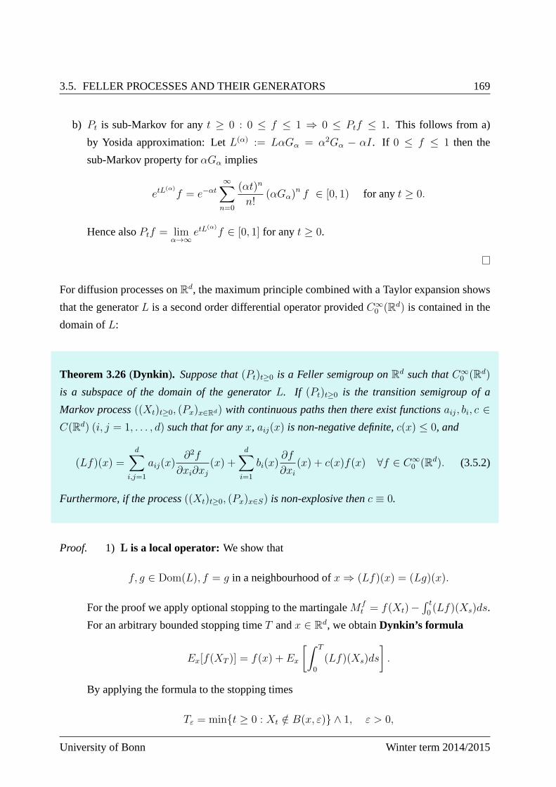
3.5. FELLER PROCESSES AND THEIR GENERATORS 169
b) Pt is sub-Markov for anyt ≥ 0 : 0 ≤ f ≤ 1 ⇒ 0 ≤ Ptf ≤ 1. This follows from a)
by Yosida approximation: LetL(α) := LαGα = α2Gα − αI. If 0 ≤ f ≤ 1 then the
sub-Markov property forαGα implies
etL(α)
f = e−αt
∞∑
n=0
(αt)n
n!(αGα)
n f ∈ [0, 1) for anyt ≥ 0.
Hence alsoPtf = limα→∞
etL(α)f ∈ [0, 1] for anyt ≥ 0.
For diffusion processes onRd, the maximum principle combined with a Taylor expansion shows
that the generatorL is a second order differential operator providedC∞0 (Rd) is contained in the
domain ofL:
Theorem 3.26(Dynkin ). Suppose that(Pt)t≥0 is a Feller semigroup onRd such thatC∞0 (Rd)
is a subspace of the domain of the generatorL. If (Pt)t≥0 is the transition semigroup of a
Markov process((Xt)t≥0, (Px)x∈Rd) with continuous paths then there exist functionsaij, bi, c ∈C(Rd) (i, j = 1, . . . , d) such that for anyx, aij(x) is non-negative definite,c(x) ≤ 0, and
(Lf)(x) =d∑
i,j=1
aij(x)∂2f
∂xi∂xj(x) +
d∑
i=1
bi(x)∂f
∂xi(x) + c(x)f(x) ∀f ∈ C∞
0 (Rd). (3.5.2)
Furthermore, if the process((Xt)t≥0, (Px)x∈S) is non-explosive thenc ≡ 0.
Proof. 1) L is a local operator: We show that
f, g ∈ Dom(L), f = g in a neighbourhood ofx⇒ (Lf)(x) = (Lg)(x).
For the proof we apply optional stopping to the martingaleM ft = f(Xt)−
´ t
0(Lf)(Xs)ds.
For an arbitrary bounded stopping timeT andx ∈ Rd, we obtainDynkin’s formula
Ex[f(XT )] = f(x) + Ex
[ˆ T
0
(Lf)(Xs)ds
].
By applying the formula to the stopping times
Tε = mint ≥ 0 : Xt /∈ B(x, ε) ∧ 1, ε > 0,
University of Bonn Winter term 2014/2015
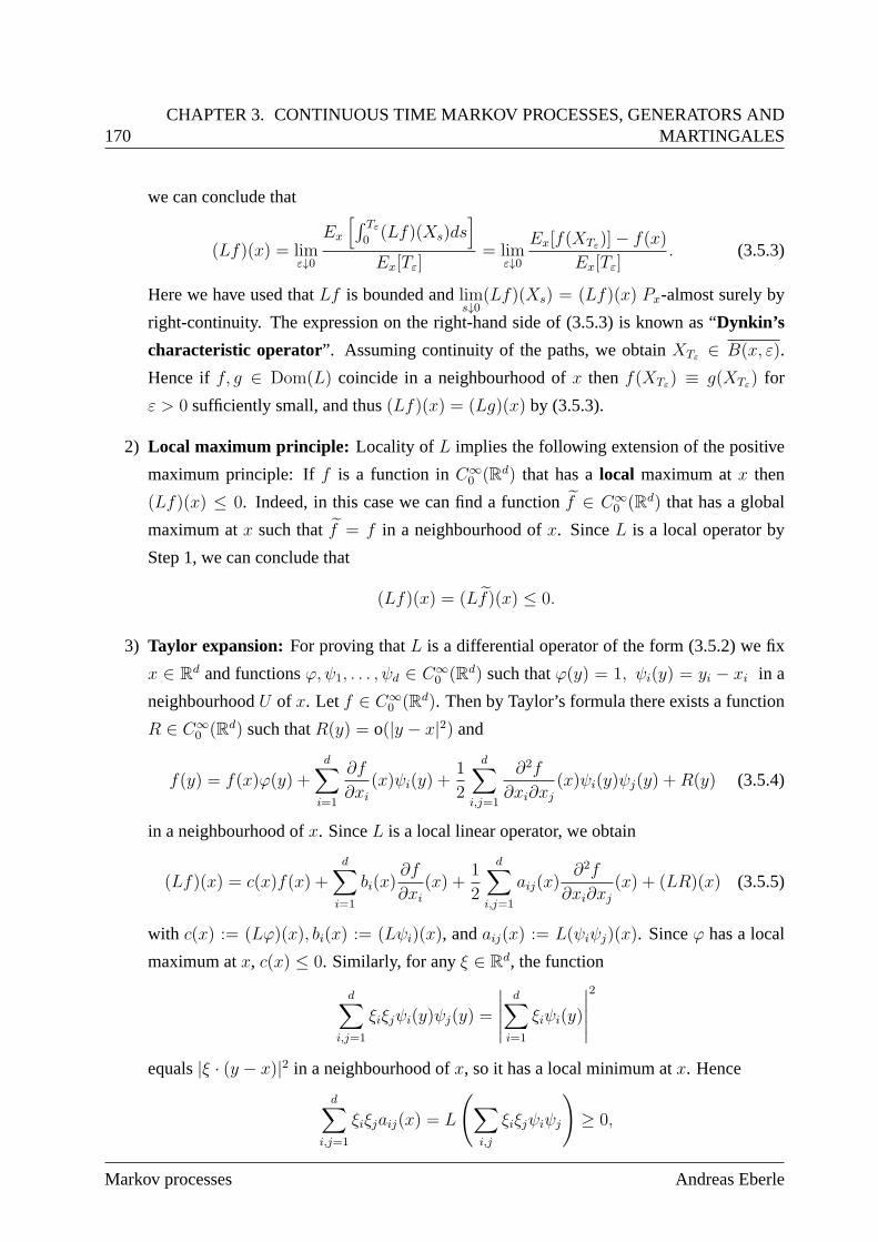
170CHAPTER 3. CONTINUOUS TIME MARKOV PROCESSES, GENERATORS AND
MARTINGALES
we can conclude that
(Lf)(x) = limε↓0
Ex
[´ Tε
0(Lf)(Xs)ds
]
Ex[Tε]= lim
ε↓0
Ex[f(XTε)]− f(x)
Ex[Tε]. (3.5.3)
Here we have used thatLf is bounded andlims↓0
(Lf)(Xs) = (Lf)(x) Px-almost surely by
right-continuity. The expression on the right-hand side of(3.5.3) is known as “Dynkin’s
characteristic operator”. Assuming continuity of the paths, we obtainXTε ∈ B(x, ε).
Hence iff, g ∈ Dom(L) coincide in a neighbourhood ofx thenf(XTε) ≡ g(XTε) for
ε > 0 sufficiently small, and thus(Lf)(x) = (Lg)(x) by (3.5.3).
2) Local maximum principle: Locality of L implies the following extension of the positive
maximum principle: Iff is a function inC∞0 (Rd) that has alocal maximum atx then
(Lf)(x) ≤ 0. Indeed, in this case we can find a functionf ∈ C∞0 (Rd) that has a global
maximum atx such thatf = f in a neighbourhood ofx. SinceL is a local operator by
Step 1, we can conclude that
(Lf)(x) = (Lf)(x) ≤ 0.
3) Taylor expansion: For proving thatL is a differential operator of the form (3.5.2) we fix
x ∈ Rd and functionsϕ, ψ1, . . . , ψd ∈ C∞0 (Rd) such thatϕ(y) = 1, ψi(y) = yi − xi in a
neighbourhoodU of x. Let f ∈ C∞0 (Rd). Then by Taylor’s formula there exists a function
R ∈ C∞0 (Rd) such thatR(y) = o(|y − x|2) and
f(y) = f(x)ϕ(y) +d∑
i=1
∂f
∂xi(x)ψi(y) +
1
2
d∑
i,j=1
∂2f
∂xi∂xj(x)ψi(y)ψj(y) +R(y) (3.5.4)
in a neighbourhood ofx. SinceL is a local linear operator, we obtain
(Lf)(x) = c(x)f(x) +d∑
i=1
bi(x)∂f
∂xi(x) +
1
2
d∑
i,j=1
aij(x)∂2f
∂xi∂xj(x) + (LR)(x) (3.5.5)
with c(x) := (Lϕ)(x), bi(x) := (Lψi)(x), andaij(x) := L(ψiψj)(x). Sinceϕ has a local
maximum atx, c(x) ≤ 0. Similarly, for anyξ ∈ Rd, the function
d∑
i,j=1
ξiξjψi(y)ψj(y) =
∣∣∣∣∣
d∑
i=1
ξiψi(y)
∣∣∣∣∣
2
equals|ξ · (y − x)|2 in a neighbourhood ofx, so it has a local minimum atx. Hence
d∑
i,j=1
ξiξjaij(x) = L
(∑
i,j
ξiξjψiψj
)≥ 0,
Markov processes Andreas Eberle
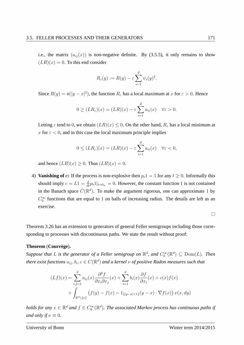
3.5. FELLER PROCESSES AND THEIR GENERATORS 171
i.e., the matrix(aij(x)) is non-negative definite. By (3.5.5), it only remains to show
(LR)(x) = 0. To this end consider
Rε(y) := R(y)− εd∑
i=1
ψi(y)2.
SinceR(y) = o(|y − x|2), the functionRε has a local maximum atx for ε > 0. Hence
0 ≥ (LRε)(x) = (LR)(x)− εd∑
i=1
aii(x) ∀ε > 0.
Lettingε tend to0, we obtain(LR)(x) ≤ 0. On the other hand,Rε has a local minimum at
x for ε < 0, and in this case the local maximum principle implies
0 ≤ (LRε)(x) = (LR)(x)− ε
d∑
i=1
aii(x) ∀ε < 0,
and hence(LR)(x) ≥ 0. Thus(LR)(x) = 0.
4) Vanishing of c: If the process is non-explosive thenpt1 = 1 for anyt ≥ 0. Informally this
should implyc = L1 = ddtpt1|t=0+ = 0. However, the constant function1 is not contained
in the Banach spaceC(Rd). To make the argument rigorous, one can approximate1 by
C∞0 functions that are equal to1 on balls of increasing radius. The details are left as an
exercise.
Theorem 3.26 has an extension to generators of general Feller semigroups including those corre-
sponding to processes with discontinuous paths. We state the result without proof:
Theorem (Courrège).
Suppose thatL is the generator of a Feller semigroup onRd, andC∞0 (Rd) ⊆ Dom(L). Then
there exist functionsaij, bi, c ∈ C(Rd) and a kernelν of positive Radon measures such that
(Lf)(x) =d∑
i,j=1
aij(x)∂2f
∂xi∂xj(x) +
d∑
i=1
bi(x)∂f
∂xi(x) + c(x)f(x)
+
ˆ
Rd\x
(f(y)− f(x)− 1|y−x|<1(y − x) · ∇f(x)
)ν(x, dy)
holds for anyx ∈ Rd andf ∈ C∞0 (Rd). The associated Markov process has continuous paths if
and only ifν ≡ 0.
University of Bonn Winter term 2014/2015
172CHAPTER 3. CONTINUOUS TIME MARKOV PROCESSES, GENERATORS AND
MARTINGALES
For transition semigroups of Lévy processes (i.e., processes with independent and stationary
increments), the coefficientsaij, bi, c, and the measureν do not depend onx. In this case, the
theorem is a consequence of the Lévy-Khinchin representation that is derived in the Stochastic
Analysis course [9].
3.6 Limits of martingale problems
Limits of martingale problems occur frequently in theoretical and applied probability. Exam-
ples include the approximation of Brownian motion by random walks and, more generally, the
convergence of Markov chains to diffusion limits, the approximation of Feller processes by jump
processes, the approximation of solutions of stochastic differential equations by solutions to more
elementary SDEs or by processes in discrete time, the construction of processes on infinite-
dimensional or singular state spaces as limits of processeson finite-dimensional or more regular
state spaces etc. A general and frequently applied approachto this type of problems can be
summarized in the following scheme:
1. Write down generatorsLn of the approximating processes and identify a limit generatorL(on an appropriate collection of test functions) such thatLn → L in an appropriate sense.
2. Prove tightness for the sequence(Pn) of laws of the solutions to the approximating martin-
gale problems. Then extract a weakly convergent subsequence.
3. Prove that the limit solves the martingale problem for thelimit generator.
4. Identify the limit process.
The technically most demanding steps are usually 2 and 4. Notice that Step 4 involves a unique-
ness statement. Since uniqueness for solutions of martingale problems is often difficult to estab-
lish (and may not hold!), the last step can not always be carried out. In this case, there may be
different subsequential limits of the sequence(Pn).
3.6.1 Weak convergence of stochastic processes
An excellent reference on this subject is the book by Billingsley [2]. LetS be a polish space. We
fix a metricd onS such that(S, d) is complete and separable. We consider the laws of stochastic
processes either on the spaceC = C([0,∞), S) of continuous functionsx : [0,∞) → S or on
Markov processes Andreas Eberle
3.6. LIMITS OF MARTINGALE PROBLEMS 173
the spaceD = D([0,∞), S) consisting of all càdlàg functionsx : [0,∞) → S. The spaceC is
again a polish space w.r.t. the topology of uniform convergence on compact time intervals:
xnC→ x :⇔ ∀T ∈ R+ : xn → x uniformly on[0, T ].
On càdlàg functions, uniform convergence is too restrictive for our purposes. For example, the
indicator functions1[0,1+n−1) do not converge uniformly to1[0,1) asn → ∞. Instead, we endow
the spaceD with the Skorokhod topology:
Definition (Skorokhod topology). A sequence of functionsxn ∈ D is said toconverge to a
limit x ∈ D in the Skorokhod topologyif and only if for anyT ∈ R+ there exist continuous and
strictly increasing mapsλn : [0, T ] → [0, T ] (n ∈ N) such that
xn(λn(t)) → x(t) and λn(t) → t uniformly on[0, T ].
It can be shown that the Skorokhod spaceD is again a polish space, cf. [2]. Furthermore, the
Borelσ-algebras on bothC andD are generated by the projectionsXt(x) = x(t), t ∈ R+.
Let (Pn)n∈N be a sequence of probability measures (laws of stochastic processes) onC,D re-
spectively. By Prokhorov’s Theorem, every subsequence of(Pn) has a weakly convergent subse-
quence provided(Pn) is tight. Here tightness means that for everyε > 0 there exists a relatively
compact subsetK ⊆ C, K ⊆ D respectively, such that
supn∈N
Pn[Kc] ≤ ε.
To verify tightness we need a characterization of the relatively compact subsets of the function
spacesC andD. In the case ofC such a characterization is the content of the classical Arzelà-
Ascoli Theorem. This result has been extended to the spaceD by Skorokhod. To state both
results we define the modulus of continuity of a functionx ∈ C on the interval[0, T ] by
ωδ,T (x) = sups,t∈[0,T ]
|s−t|≤δ
d(x(s), x(t)).
Forx ∈ D we define a modification ofωδ,T by
ω′δ,T (x) = inf
0=t0<t1<···<tn−1<T≤tn
|ti−ti−1|>δ
maxi
sups,t∈[ti−1,ti)
d(x(s), x(t)).
As δ ↓ 0, ωδ,T (x) → 0 for anyx ∈ C andT > 0. For a discontinuous functionx ∈ D, ωδ,T (x)
does not converge to0. However, the modified quantityω′δ,T (x) again converges to0, since the
partition in the infimum can be chosen in such a way that jumps of size greater than some constant
ε occur only at partition points and are not taken into accountin the inner maximum.
University of Bonn Winter term 2014/2015
174CHAPTER 3. CONTINUOUS TIME MARKOV PROCESSES, GENERATORS AND
MARTINGALES
Exercise(Modulus of continuity and Skorokhod modulus). Let x ∈ D.
1) Show thatlimδ↓0
ωδ,T (x) = 0 for anyT ∈ R+ if and only if x is continuous.
2) Prove thatlimδ↓0
ω′δ,T (x) = 0 for anyT ∈ R+.
Theorem 3.27(Arzelà-Ascoli, Skorokhod). 1) A subsetK ⊆ C is relatively compact if and
only if
(i) x(0) : x ∈ K is relatively compact inS, and
(ii) supx∈K
ωδ,T (x) → 0 asδ ↓ 0 for anyT > 0.
2) A subsetK ⊆ D is relatively compact if and only if
(i) x(t) : x ∈ K is relatively compact for anyt ∈ Q+, and
(ii) supx∈K
ω′δ,T (x) → 0 asδ ↓ 0 for anyT > 0.
The proofs can be found in Billingsley [2] or Ethier/Kurtz [11]. By combining Theorem 3.27
with Prokhorov’s Theorem, one obtains:
Corollary 3.28 (Tightness of probability measures on function spaces).
1) A subsetPn : n ∈ N ofP(C) is relatively compact w.r.t. weak convergence if and only if
(i) For any ε > 0, there exists a compact setK ⊆ S such that
supn∈N
Pn[X0 /∈ K] ≤ ε, and
(ii) For any T ∈ R+,
supn∈N
Pn[ωδ,T > ε] → 0 asδ ↓ 0.
2) A subsetPn : n ∈ N ofP(D) is relatively compact w.r.t. weak convergence if and only if
(i) For any ε > 0 andt ∈ R+ there exists a compact setK ⊆ S such that
supn∈N
Pn[Xt /∈ K] ≤ ε, and
Markov processes Andreas Eberle
3.6. LIMITS OF MARTINGALE PROBLEMS 175
(ii) For any T ∈ R+,
supn∈N
Pn[ω′δ,T > ε] → 0 asδ ↓ 0.
In the sequel we restrict ourselves to convergence of stochastic processes with continuous paths.
We point out, however, that many of the arguments can be carried out (with additional difficulties)
for processes with jumps if the space of continuous functions is replaced by the Skorokhod space.
A detailed study of convergence of martingale problems for discontinuous Markov processes can
be found in Ethier/Kurtz [11].
To apply the tightness criterion we need upper bounds for theprobabilitiesPn[ωδ,T > ε]. To
this end we observe thatωδ,T ≤ ε if
supt∈[0,δ]
d(Xkδ+t, Xkδ) ≤ε
3for anyk ∈ Z+ such thatkδ < T.
Therefore, we can estimate
Pn[ωδ,T > ε] ≤⌊T/δ⌋∑
k=0
Pn
[supt≤δ
d(Xkδ+t, Xkδ) > ε/3
]. (3.6.1)
Furthermore, onRn we can bound the distancesd(Xkδ+t, Xkδ) by the sum of the differences
|X ikδ+t −X i
kδ| of the componentsX i, i = 1, . . . , d. The suprema can then be controlled by ap-
plying a semimartingale decomposition and the maximal inequality to the component processes.
3.6.2 From Random Walks to Brownian motion
As a first application of the tightness criterion we prove Donsker’s invariance principle stating
that rescaled random walks with square integrable increments converge in law to a Brownian
motion. In particular, this is a way (although not the easiest one) to prove that Brownian motion
exists. Let(Yi)i∈N be a sequence of i.i.d. square-integrable random variableson a probability
space(Ω,A, P ) with E[Yi] = 0 andVar[Yi] = 1, and consider the random walk
Sn =n∑
i=1
Yi (n ∈ N).
We rescale diffusively, i.e., by a factorn in time and a factor√n in space, and define
X(n)t :=
1√nSnt for t ∈ R+ such thatnt ∈ Z.
In between the partition pointst = k/n, k ∈ Z+, the process(X(n)t ) is defined by linear interpo-
lation so thatX(n) has continuous paths.
University of Bonn Winter term 2014/2015
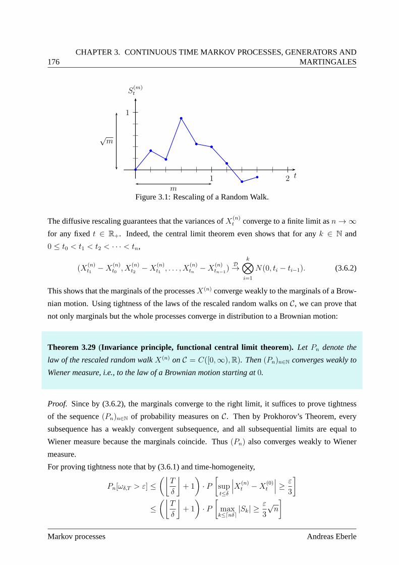
176CHAPTER 3. CONTINUOUS TIME MARKOV PROCESSES, GENERATORS AND
MARTINGALES
1
1 2
√m
m
S(m)t
t
Figure 3.1: Rescaling of a Random Walk.
The diffusive rescaling guarantees that the variances ofX(n)t converge to a finite limit asn→ ∞
for any fixedt ∈ R+. Indeed, the central limit theorem even shows that for anyk ∈ N and
0 ≤ t0 < t1 < t2 < · · · < tn,
(X(n)t1 −X
(n)t0 , X
(n)t2 −X
(n)t1 , . . . , X
(n)tn −X
(n)tn−1
)D→
k⊗
i=1
N(0, ti − ti−1). (3.6.2)
This shows that the marginals of the processesX(n) converge weakly to the marginals of a Brow-
nian motion. Using tightness of the laws of the rescaled random walks onC, we can prove that
not only marginals but the whole processes converge in distribution to a Brownian motion:
Theorem 3.29(Invariance principle, functional central limit theorem ). Let Pn denote the
law of the rescaled random walkX(n) onC = C([0,∞),R). Then(Pn)n∈N converges weakly to
Wiener measure, i.e., to the law of a Brownian motion startingat 0.
Proof. Since by (3.6.2), the marginals converge to the right limit,it suffices to prove tightness
of the sequence(Pn)n∈N of probability measures onC. Then by Prokhorov’s Theorem, every
subsequence has a weakly convergent subsequence, and all subsequential limits are equal to
Wiener measure because the marginals coincide. Thus(Pn) also converges weakly to Wiener
measure.
For proving tightness note that by (3.6.1) and time-homogeneity,
Pn[ωδ,T > ε] ≤(⌊
T
δ
⌋+ 1
)· P[supt≤δ
∣∣∣X(n)t −X
(0)t
∣∣∣ ≥ ε
3
]
≤(⌊
T
δ
⌋+ 1
)· P[maxk≤⌈nδ⌉
|Sk| ≥ε
3
√n
]
Markov processes Andreas Eberle
3.6. LIMITS OF MARTINGALE PROBLEMS 177
for anyε, δ > 0, T ∈ R+ andn ∈ N. By Corollary 3.28, tightness holds if the probability on the
right hand side is of order o(S) uniformly in n, i.e., if
lim supn→∞
P
[maxk≤m
|Sk| ≥ε
3
√m√δ
]= o(δ). (3.6.3)
For the simple random walk, this follows from the reflection principle and the central limit theo-
rem as
P
[maxk≤m
Sk ≥ε
3
√m√δ
]≤ P
[|Sm| ≥
ε
3
√m√δ
]m↑∞−→ N(0, 1)
[|x| ≥ ε
3√δ
],
cf. e.g. [8]. For general random walks one can show with some additional arguments that (3.6.3)
also holds, see e.g. Billingsley [2].
In the proof of Donsker’s Theorem, convergence of the marginals was a direct consequence of the
central limit theorem. In more general situations, other methods are required to identify the limit
process. Therefore, we observe that instead of the central limit theorem, we could have also used
the martingale problem to identify the limit as a Brownian motion. Indeed, the rescaled random
walk(X
(n)k/n
)k∈Z+
is a Markov chain (in discrete time) with generator
(L(n)f)(x) =
ˆ(f
(x+
z√n
)− f(x)
)ν(dz)
whereν is the distribution of the incrementsYi = Si − Si−1. It follows that w.r.t.Pn, the process
f(Xt)−nt−1∑
i=0
(nL(n)f)(Xi/n) ·1
n, t =
k
nwith k ∈ Z+,
is a martingale for any functionf ∈ C∞b (R). Asn→ ∞,
f
(x+
z√n
)− f(x) = f ′(x) ·
ˆ
z√nν(dz) +
1
2f ′′(x)
ˆ
z2
nν(dz) + o(n−1)
=1
2nf ′′(x) + o(n−1)
by Taylor, and
(nL(n)f)(x) → 1
2f ′′(x) uniformly.
Therefore, one can conclude that the process
f(Xt)−ˆ t
0
1
2f ′′(Xs)ds
is a martingale underP∞ for any weak limit point of the sequence(Pn). Uniqueness of the
martingale problem then implies thatP∞ is the law of a Brownian motion.
Exercise (Martingale problem proof of Donsker’s Theorem). Carry out carefully the argu-
ments sketched above and give an alternative proof of Donsker’s Theorem that avoids application
of the central limit theorem.
University of Bonn Winter term 2014/2015
178CHAPTER 3. CONTINUOUS TIME MARKOV PROCESSES, GENERATORS AND
MARTINGALES
3.6.3 Regularity and tightness for solutions of martingale problems
We will now extend the martingale argument for proving Donsker’s Theorem that has been
sketched above to limits of general martingale problems on the spaceC = C([0,∞), S) where
S is a polish space. We first introduce a more general frameworkthat allows to include non-
Markovian processes. The reason is that it is sometimes convenient to approximate Markov
processes by processes with a delay, see the proof of Theorem3.33 below.
Suppose thatA is a linear subspace ofFb(S), and
f 7→ (Ltf)t≥0
is a linear map defined onA such that
(t, x) 7→ (Ltf)(x) is a function inL2([0, T ]× C, λ⊗ P )
for anyT ∈ R+ andf ∈ A. The main example is still the one of time-homogeneous Markov
processes with generatorL where we set
Ltf := (Lf)(Xt).
We say that the canonical processXt(ω) = ω(t) solves the martingale problemMP(Lt,A)
w.r.t. a probability measureP onC iff
M ft = f(Xt)− f(X0)−
ˆ t
0
Lrf dr
is a martingale underP for anyf ∈ A. Note that for0 ≤ s ≤ t,
f(Xt)− f(Xs) =M ft −M f
s +
ˆ t
s
Lrf dr. (3.6.4)
Therefore, martingale inequalities can be used to control the regularity of the processf(Xt). As a
first step in this direction we compute the angle-bracket process〈M f〉, i.e., the martingale part in
the Doob-Meyer decomposition of(M f )2. Since we are considering processes with continuous
paths, the angle-bracket process coincides with the quadratic variation[M f ]. The next theorem,
however, is also valid for processes with jumps where〈M f〉 6= [M f ]:
Markov processes Andreas Eberle
3.6. LIMITS OF MARTINGALE PROBLEMS 179
Theorem 3.30(Angle-bracket process for solutions of martingale problems). Let f, g ∈ Asuch thatf · g ∈ A. Then
M ft ·M g
t = N f,gt +
ˆ t
0
Γr(f, g) dr for anyt ≥ 0,
whereN f,g is a martingale, and
Γt(f, g) = Lt(f · g)− f(Xt)Ltg − g(Xt)Ltf.
Thus
〈M f ,M g〉t =ˆ t
0
Γr(f, g) dr.
Example (Time-homogeneous Markov processes, Carré du champ operator).
HereLtf = (Lf)(Xt), and therefore
Γt(f, g) = Γ(f, g)(Xt),
whereΓ : A×A → F(S) is theCarré du champ operator defined by
Γ(f, g) = L(f · g)− fLg − gLf.
If S = Rd,A is a subset ofC∞(Rd), and
(Lf)(x) = 1
2
d∑
i,j=1
aij(x)∂2f
∂xi∂xj(x) +
d∑
i=1
bi(x)∂f
∂xi(x) ∀f ∈ A
with measurable coefficientsaij, bi then
Γ(f, g)(x) =d∑
i,j=1
aij(x)∂f
∂xi(x)
∂g
∂xj(x) ∀f, g ∈ A.
In particular, foraij ≡ δij ,Γ(f, f) = |∇f |2 which explains the name “carré du champ” (= square
field) operator. For general symmetric coefficientsaij with det(aij) > 0, the carré du champ is
the square of the gradient w.r.t. the intrinsic metric(gij) = (aij)−1:
Γ(f, f) = ‖ gradg f‖2g.
Proof of Theorem 3.30.We may assumef = g, the general case follows by polarization. We
write “X ∼s Y ” if E[X|Fs] = E[Y |Fs] almost surely. To prove the claim we have to show that
for 0 ≤ s ≤ t andf ∈ A,
(M ft )
2 − (M fs )
2 ∼ˆ t
s
Γr(f, f) dr.
University of Bonn Winter term 2014/2015
180CHAPTER 3. CONTINUOUS TIME MARKOV PROCESSES, GENERATORS AND
MARTINGALES
SinceM f is a square-integrable martingale, we have
(M ft )
2 − (M fs )
2 ∼s (Mft −M f
s )2 =
(f(Xt)− f(Xs)−
ˆ t
s
Lrf dr
)2
= (f(Xt)− f(Xs))2 − 2(f(Xt)− f(Xs))
ˆ t
s
Lrf dr +
(ˆ t
s
Lrf dr
)2
= I + II + III + IV
where
I := f(Xt)2 − f(Xs)
2 ∼s
ˆ t
s
Lrf2 dr,
II := −2f(Xs)
(f(Xt)− f(Xs)−
ˆ t
s
Lrf dr
)∼s 0,
III := −2f(Xt)
ˆ t
s
Lrf dr = −2
ˆ t
s
f(Xt)Lrf dr, and
IV :=
(ˆ t
s
Lrf dr
)2
= 2
ˆ t
s
ˆ t
r
Lrf Luf dudr.
Noting thatf(Xt)Lrf ∼r
(f(Xr) +
´ t
rLuf du
)Lrf , we see that fors ≤ r ≤ t also the condi-
tional expectations givenFs of these terms agree, and therefore
III ∼s −2
ˆ t
s
f(Xr)Lrf dr − 2
ˆ t
s
ˆ t
r
Lrf Luf dudr.
Hence in total we obtain
(M ft )
2 − (M fs )
2 ∼s
ˆ t
s
Lrf2 dr − 2
ˆ t
s
f(Xr)Lrf dr =
ˆ t
s
Γrf dr.
We can now derive a bound for the modulus of continuity off(Xt) for a functionf ∈ A. Let
ωfδ,T := ωδ,T (f X), V f
s,t := supr∈[s,t]
|f(Xr)− f(Xs)|.
Lemma 3.31(Modulus of continuity of solutions to martingale problems). For p ∈ [2,∞)
there exist universal constantsCp, Cp ∈ (0,∞) such that the following bounds hold for any
solution (Xt, P ) of a martingale problem as above and for any functionf ∈ A such that the
processf(Xt) has continuous paths:
1) For any0 ≤ s ≤ t,
‖V fs,t‖Lp(P ) ≤ Cp(t− s)1/2 sup
r∈[s,t]‖Γr(f, f)‖1/2Lp/2(P )
+ (t− s) supr∈[s,t]
‖Lrf‖Lp(P ).
Markov processes Andreas Eberle
3.6. LIMITS OF MARTINGALE PROBLEMS 181
2) For anyδ, ε, T ∈ (0,∞),
P[ωfδ,T ≥ ε
]≤ Cp ε
−p
(1 +
⌊T
δ
⌋)·(δp/2 sup
r≤T‖Γr(f, f)‖p/2Lp/2(P )
+ δp supr≤t
‖Lrf‖Lp(P )
).
Proof. 1) By (3.6.4),
V fs,t ≤ sup
r∈[s,t]|M f
r −M fs |+
ˆ t
s
|Luf | du.
Sincef(Xt) is continuous,M f is a continuous martingale. Therefore, byBurkholder’s
inequality,
∥∥∥ supr∈[s,t]
∣∣M fr −M f
s
∣∣∥∥∥Lp(P )
≤ Cp
∥∥〈M f〉t − 〈M f〉s∥∥1/2Lp/2(P )
= Cp
∥∥∥∥ˆ t
s
Γr(f, f) dr
∥∥∥∥1/2
Lp/2(P )
≤ Cp(t− s)1/2 supr∈[s,t]
‖Γr(f, f)‖1/2Lp/2(P ).
Forp = 2, Burkholder’s inequality reduces to the usual maximal inequality for martingales
- a proof forp > 2 can be found in many stochastic analysis textbooks, cf. e.g.[9].
2) We have already remarked above that the modulus of continuity ωfδ,T can be controlled by
bounds forV fs,t on intervals[s, t] of lengthδ. Here we obtain
P[ωfδ,T ≥ ε
]≤
⌊T/δ⌋∑
k=0
P[V fkδ,(k+1)δ ≥ ε/3
]
≤⌊T/δ⌋∑
k=0
(3
ε
)p ∥∥∥V fkδ,(k+1)δ
∥∥∥p
Lp(P ).
The estimate in 2) now follows from 1).
Remark. 1) The right-hand side in 2) converges to0 asδ ↓ 0 if the suprema are finite and
p > 2.
2) If f(Xt) is not continuous then the assertion still holds forp = 2 but not for p > 2.
The reason is that Burkholder’s inequality for discontinuous martingalesMt is a bound in
terms of the quadratic variation[M ]t and not in terms of the angle bracket process〈M〉t.For continuous martingales,〈M〉t = [M ]t.
University of Bonn Winter term 2014/2015
182CHAPTER 3. CONTINUOUS TIME MARKOV PROCESSES, GENERATORS AND
MARTINGALES
Example (Stationary Markov process).
If (Xt, P ) is a stationary Markov process with generator extending(L,A) and stationary distri-
butionXt ∼ µ thenLtf = (Lf)(Xt), Γt(f, f) = Γ(f, f)(Xt), and therefore
‖Ltf‖Lp(P ) = ‖Lf‖Lp(µ), ‖Γt(f, f)‖Lp/2(P ) = ‖Γ(f, f)‖Lp/2(µ) for anyt ≥ 0.
3.6.4 Construction of diffusion processes
The results above can be applied to prove the existence of diffusion processes generated by second
order differential operators with continuous coefficientsonRd. The idea is to obtain the law of the
process as a weak limit of laws of processes with piecewise constant coefficients. The latter can
be constructed from Brownian motion in an elementary way. Thekey step is again to establish
tightness of the approximating laws.
Theorem 3.32(Existence of diffusions inRd). For 1 ≤ i, j ≤ d let aij, bi ∈ Cb(R+ ×Rd) such
thataij = aji. Then for anyx ∈ Rd there exists a probability measurePx onC([0,∞),Rd) such
that the canonical process(Xt, Px) solves the martingale problem for the operator
Ltf =1
2
d∑
i,j=1
aij(t,Xt)∂2f
∂xi∂xj(Xt) +
d∑
i=1
bi(t,Xt)∂f
∂xi(Xt)
with domain
A =
f ∈ C∞(Rd) :
∂f
∂xi∈ C∞
b (Rd) for i = 1, . . . , d
and initial conditionPx[X0 = x] = 1.
Remark (Connections to SDE results). 1) If the coefficients are locally Lipschitz continu-
ous then the existence of a diffusion process follows more easily from the Itô existence and
uniqueness result for stochastic differential equations.The point is, however, that variants
of the general approach presented here can be applied in manyother situations as well.
2) The approximations used in the proof below correspond to Euler discretizations of the
associated SDE.
Proof. 1) We first define the approximating generators and constructprocesses solving the
corresponding martingale problems. Forn ∈ N let
a(n)ij (t,X) = aij(⌊t⌋n, X⌊t⌋n), bni (t,X) = bi(⌊t⌋n, X⌊t⌋n)
Markov processes Andreas Eberle
3.6. LIMITS OF MARTINGALE PROBLEMS 183
where⌊t⌋n := maxs ∈ 1
nZ : s ≤ t
, i.e., for t ∈
[kn, k+1
n
), we freeze the coefficients at
their value at timekn. Then the martingale problem for
L(n)t f =
1
2
d∑
i,j=1
a(n)ij (t,X)
∂2f
∂xi∂xj(Xt) +
d∑
i=1
b(n)i (t,X)
∂f
∂xi(Xt)
can be solved explicitly. Indeed let(Bt) be a Brownian motion onRd defined on a prob-
ability space(Ω,A, P ), and letσ : R+ × Rd → Rd×d be measurable such thatσσT = a.
Then the processX(n)t defined recursively by
X(n)0 = x, X
(n)t = X
(n)k/n+σ
(k
n,X
(n)k/n
)(Bt−Bk/n)+b
(k
n,X
(n)k/n
)k
nfor t ∈
[0,
1
n
],
solves the martingale problem for(L(n)t ,A) with initial conditionδx. Hence the canonical
process(Xt) onC([0,∞),Rd) solves the same martingale problem w.r.t.
P (n) = P (X(n)
)−1.
2) Next we prove tightness of the sequenceP (n) : n ∈ N. For i = 1, . . . , d let fi(x) := xi.
Since|x− y| ≤∑di=1 |fi(x)− fi(y)| for anyx, y ∈ Rd, we have
ωδ,T ≤d∑
i=1
ωfiδ,T for anyδ, T ∈ (0,∞).
Furthermore, the functions
L(n)t fi = b
(n)i (t,X) and Γ
(n)t (fi, fi) = a
(n)ii (t,X)
are uniformly bounded since the coefficientsaij andbi are bounded functions. Therefore,
for anyε, T ∈ (0,∞),
P (n) [ωδ,T ≥ ε] ≤d∑
i=1
P (n)[ωfiδ,T ≥ ε/d
]→ 0
uniformly in n asδ ↓ 0 by Lemma 3.31.
Hence by Theorem 3.29, the sequenceP (n) : n ∈ N is relatively compact, i.e., there
exists a subsequential limitP ∗ w.r.t. weak convergence.
3) It only remains to show that(Xt, P∗) solves the limiting martingale problem. We know that
(Xt, P(n)) solves the martingale problem for(L(n)
t ,A) with initial law δx. In particular,
E(n)
[(f(Xt)− f(Xs)−
ˆ t
s
L(n)r f dr
)g(Xs1 , . . . , Xsk)
]= 0
University of Bonn Winter term 2014/2015
184CHAPTER 3. CONTINUOUS TIME MARKOV PROCESSES, GENERATORS AND
MARTINGALES
for any0 ≤ s1 < s2 < · · · < sk ≤ s ≤ t andg ∈ Cb(Rk·d). The assumptions imply that
L(n)r f → Lrf pointwise asn → ∞, andL(n)
r f is uniformly bounded. This can be used
to show that(Xt, P∗) solves the martingale problem for(Lt, f) - the details are left as an
exercise.
Remark (Uniqueness). The assumptions in Theorem 3.32 are too weak to guarantee uniqueness
of the solution. For example, the ordinary differential equation dx = b(x)dt does not have a
unique solution withx0 = 0 whenb(x) =√x. As a consequence, one can show that the trivial
solution to the martingale problem for the operatorb(x) ddx
on R1 is not the only solution with
initial law δ0. A uniqueness theorem of Stroock and Varadhan states that the martingale problem
has a unique solution for every initial law if the matrixa(x) is strictly positive definite for each
x, and the growth of the coefficients as|x| → ∞ is at most of orderaij(x) = O(|x|2) and
bi(x) = O(|x|), cf. (24.1) in Roger&Williams II [31] for a sketch of the proof.
3.6.5 The general case
We finally state a general result on limits of martingale problems for processes with continuous
paths. Let(P (n))n∈N be a sequence of probability measures onC([0,∞), S) whereS is a polish
space. Suppose that the canonical process(Xt, P(n)) solves the martingale problem for(L(n)
t ,A)
whereA is a dense subspace ofCb(S) such thatf 2 ∈ A wheneverf ∈ A.
Theorem 3.33.Suppose that the following conditions hold:
(i) Compact containment:For anyT ∈ R+ andγ > 0 there exists a compact setK ⊆ S such
that
P (n)[∃ t ∈ [0, T ] : Xt /∈ K
]≤ γ for anyn ∈ N.
(ii) Uniform Lp bound: There existsp > 2 such that for anyT ∈ R+,
supn∈N
supt≤T
(∥∥∥Γ(n)t (f, f)
∥∥∥Lp/2(P (n))
+∥∥∥L(n)
t f∥∥∥Lp(P (n))
)<∞.
ThenP (n) : n ∈ N is relatively compact. Furthermore, if
(iii) Convergence of initial law:There existsµ ∈ P(S) such that
P (n) X−10
w→ µ asn→ ∞, and
Markov processes Andreas Eberle
3.6. LIMITS OF MARTINGALE PROBLEMS 185
(iv) Convergence of generators:
L(n)t f → Ltf uniformly for anyf ∈ A,
then any subsequential limit of(P (n))n∈N is a solution of the martingale problem for(Lt,A) with
initial distribution µ.
The proof, including extensions to processes with discontinuous paths, can be found in Ethier
and Kurtz [11].
University of Bonn Winter term 2014/2015
Chapter 4
Convergence to equilibrium
Additional references for this chapter: Royer [33], Malrieu[21], Bakry, Gentil, Ledoux [1]
Our goal in the following sections is to relate the long time asymptotics(t ↑ ∞) of a time-
homogeneous Markov process (respectively its transition semigroup) to its infinitesimal charac-
teristics which describe the short-time behavior(t ↓ 0):
Asymptotic properties ↔ Infinitesimal behavior, generator
t ↑ ∞ t ↓ 0
Although this is usually limited to the time-homogeneous case, some of the results can be applied
to time-inhomogeneous Markov processes by considering thespace-time process(t,Xt), which
is always time-homogeneous. On the other hand, we would liketo take into account processes
that jump instantaneously (as e.g. interacting particle systems onZd) or have continuous trajecto-
ries (diffusion-processes). In this case it is not straightforward to describe the process completely
in terms of infinitesimal characteristics, as we did for jumpprocesses. A convenient general setup
that can be applied to all these types of Markov processes is the martingale problem of Stroock
and Varadhan.
LetS be a Polish space endowed with its Borelσ-algebraS. ByFb(S) we denote the linear space
of all bounded measurable functionsf : S → R. Suppose thatA is a linear subspace ofFb(S)
such that
(A0) If µ is a signed measure onS with finite variation andˆ
f dµ = 0 ∀ f ∈ A,
thenµ = 0
186
187
Let
L : A ⊆ Fb(S) → Fb(S)
be a linear operator.
From now on we assume that we are given a right continuous time-homogeneous Markov process
((Xt)t≥0, (Ft)t≥0, (Px)x∈S) with transition semigroup(pt)t≥0 such that for anyx ∈ S, (Xt)t≥0 is
underPx a solution of the martingale problem for(L,A) with Px [X0 = x] = 1.
Let A denote the closure ofA with respect to the supremum norm. For most results derived
below, we will impose two additional assumptions:
Assumptions:
(A1) If f ∈ A, thenLf ∈ A.
(A2) There exists a linear subspaceA0 ⊆ A such that iff ∈ A0, thenptf ∈ A for all t ≥ 0, and
A0 is dense inA with respect to the supremum norm.
Example. (1). For a diffusion process inRd with continuous non-degenerated coefficients sat-
isfying an appropriate growth constraint at infinity, (A1) and (A2) hold withA0 = C∞0 (Rd),
A = S(Rd) andB = A = C∞(Rd).
(2). In general, it can be difficult to determine explicitly aspaceA0 such that (A2) holds. In
this case, a common procedure is to approximate the Markov process and its transition
semigroup by more regular processes (e.g. non-degenerate diffusions inRd), and to derive
asymptotic properties from corresponding properties of the approximands.
(3). For an interacting particle system onT Zdwith bounded transition ratesci(x, η), the condi-
tions (A1) and (A2) hold with
A0 = A =f : T Zd → R : |||f ||| <∞
where
|||f ||| =∑
x∈Zd
∆f (x), ∆f (x) = supi∈T
∣∣f(ηx,i)− f(η)∣∣ ,
cf. Liggett [18].
University of Bonn Winter term 2014/2015
188 CHAPTER 4. CONVERGENCE TO EQUILIBRIUM
Theorem (From the martingale problem to the Kolmogorov equations).
Suppose (A1) and (A2) hold. Then(pt)t≥0 induces aC0 contraction semigroup(Pt)t≥0 on the
Banach spaceB = A = A0, and the generator is an extension of(L,A). In particular, the
forward and backward equations
d
dtptf = ptLf ∀ f ∈ A
and
d
dtptf = Lptf ∀ f ∈ A0
hold.
Proof. SinceM ft is a bounded martingale with respect toPx, we obtain the integrated forward
equation by Fubini:
(ptf)(x)− f(x) = Ex[f(Xt)− f(X0)] = Ex
tˆ
0
(Lf)(Xs) ds
=
tˆ
0
(psLf)(x) ds
(4.0.1)
for all f ∈ A andx ∈ S. In particular,
‖ptf − f‖sup ≤tˆ
0
‖psLf‖sup ds ≤ t · ‖Lf‖sup → 0
ast ↓ 0 for anyf ∈ A. This implies strong continuity onB = A since eachpt is a contraction
with respect to the sup-norm. Hence by (A1) and (4.0.1),
ptf − f
t− Lf =
1
t
tˆ
0
(psLf − Lf) ds→ 0
uniformly for all f ∈ A, i.e. A is contained in the domain of the generator L of the semigroup
(Pt)t≥0 induced onB, andLf = Lf for all f ∈ A. Now the forward and the backward equations
follow from the corresponding equations for(Pt)t≥0 and Assumption (A2).
Markov processes Andreas Eberle
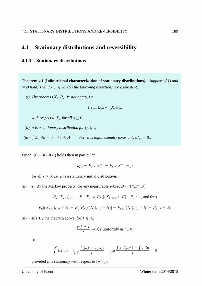
4.1. STATIONARY DISTRIBUTIONS AND REVERSIBILITY 189
4.1 Stationary distributions and reversibility
4.1.1 Stationary distributions
Theorem 4.1(Infinitesimal characterization of stationary distributio ns). Suppose (A1) and
(A2) hold. Then forµ ∈M1(S) the following assertions are equivalent:
(i) The process(Xt, Pµ) is stationary, i.e.
(Xs+t)t≥0 ∼ (Xt)t≥0
with respect toPµ for all s ≥ 0.
(ii) µ is a stationary distribution for(pt)t≥0
(iii)´
Lf dµ = 0 ∀ f ∈ A (i.e. µ is infinitesimally invariant,L∗µ = 0).
Proof. (i)⇒(ii) If (i) holds then in particular
µps = Pµ X−1s = Pµ X−1
0 = µ
for all s ≥ 0, i.e.µ is a stationary initial distribution.
(ii)⇒(i) By the Markov property, for any measurable subsetB ⊆ D(R+, S),
Pµ[(Xs+t)t≥0 ∈ B | Fs] = PXs [(Xt)t≥0 ∈ B] Pµ-a.s., and thus
Pµ[(Xs+t)t≥0 ∈ B] = Eµ[PXs((Xt)t≥0 ∈ B)] = Pµps [(Xt)t≥0 ∈ B] = Pµ[X ∈ B]
(ii)⇒(iii) By the theorem above, forf ∈ A,
ptf − f
t→ Lf uniformly ast ↓ 0,
soˆ
Lf dµ = limt↓0
´
(ptf − f) dµ
t= lim
t↓0
´
f d(µpt)−´
f dµ
t= 0
providedµ is stationary with respect to(pt)t≥0.
University of Bonn Winter term 2014/2015
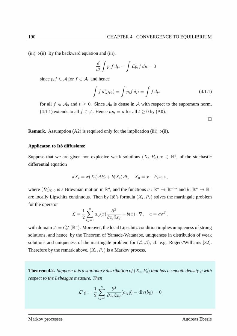
190 CHAPTER 4. CONVERGENCE TO EQUILIBRIUM
(iii)⇒(ii) By the backward equation and (iii),
d
dt
ˆ
ptf dµ =
ˆ
Lptf dµ = 0
sinceptf ∈ A for f ∈ A0 and henceˆ
f d(µpt) =
ˆ
ptf dµ =
ˆ
f dµ (4.1.1)
for all f ∈ A0 andt ≥ 0. SinceA0 is dense inA with respect to the supremum norm,
(4.1.1) extends to allf ∈ A. Henceµpt = µ for all t ≥ 0 by (A0).
Remark. Assumption (A2) is required only for the implication (iii)⇒(ii).
Applicaton to Itô diffusions:
Suppose that we are given non-explosive weak solutions(Xt, Px), x ∈ Rd, of the stochastic
differential equation
dXt = σ(Xt) dBt + b(Xt) dt, X0 = x Px-a.s.,
where(Bt)t≥0 is a Brownian motion inRd, and the functionsσ : Rn → Rn×d andb : Rn → Rn
are locally Lipschitz continuous. Then by Itô’s formula(Xt, Px) solves the martingale problem
for the operator
L =1
2
n∑
i,j=1
aij(x)∂2
∂xi∂xj+ b(x) · ∇, a = σσT ,
with domainA = C∞0 (Rn). Moreover, the local Lipschitz condition implies uniqueness of strong
solutions, and hence, by the Theorem of Yamade-Watanabe, uniqueness in distribution of weak
solutions and uniqueness of the martingale problem for(L,A), cf. e.g. Rogers/Williams [32].
Therefore by the remark above,(Xt, Px) is a Markov process.
Theorem 4.2.Supposeµ is a stationary distribution of(Xt, Px) that has a smooth densitywith
respect to the Lebesgue measure. Then
L∗ :=1
2
n∑
i,j=1
∂2
∂xi∂xj(aij)− div(b) = 0
Markov processes Andreas Eberle
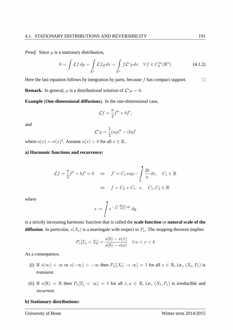
4.1. STATIONARY DISTRIBUTIONS AND REVERSIBILITY 191
Proof. Sinceµ is a stationary distribution,
0 =
ˆ
Lf dµ =
ˆ
Rn
Lf dx =
ˆ
Rn
fL∗ dx ∀ f ∈ C∞0 (Rn) (4.1.2)
Here the last equation follows by integration by parts, becausef has compact support.
Remark. In general,µ is a distributional solution ofL∗µ = 0.
Example (One-dimensional diffusions). In the one-dimensional case,
Lf =a
2f ′′ + bf ′,
and
L∗ =1
2(a)′′ − (b)′
wherea(x) = σ(x)2. Assumea(x) > 0 for all x ∈ R.
a) Harmonic functions and recurrence:
Lf =a
2f ′′ + bf ′ = 0 ⇔ f ′ = C1 exp−
•ˆ
0
2b
adx, C1 ∈ R
⇔ f = C2 + C1 · s, C1, C2 ∈ R
where
s :=
•ˆ
0
e−´ y0
2b(x)a(x)
dx dy
is a strictly increasing harmonic function that is called thescale functionor natural scale of the
diffusion. In particular,s(Xt) is a martingale with respect toPx. The stopping theorem implies
Px[Ta < Tb] =s(b)− s(x)
s(b)− s(a)∀ a < x < b
As a consequence,
(i) If s(∞) < ∞ or s(−∞) > −∞ thenPx[|Xt| → ∞] = 1 for all x ∈ R, i.e., (Xt, Px) is
transient.
(ii) If s(R) = R thenPx[Ta < ∞] = 1 for all x, a ∈ R, i.e., (Xt, Px) is irreducible and
recurrent.
b) Stationary distributions:
University of Bonn Winter term 2014/2015
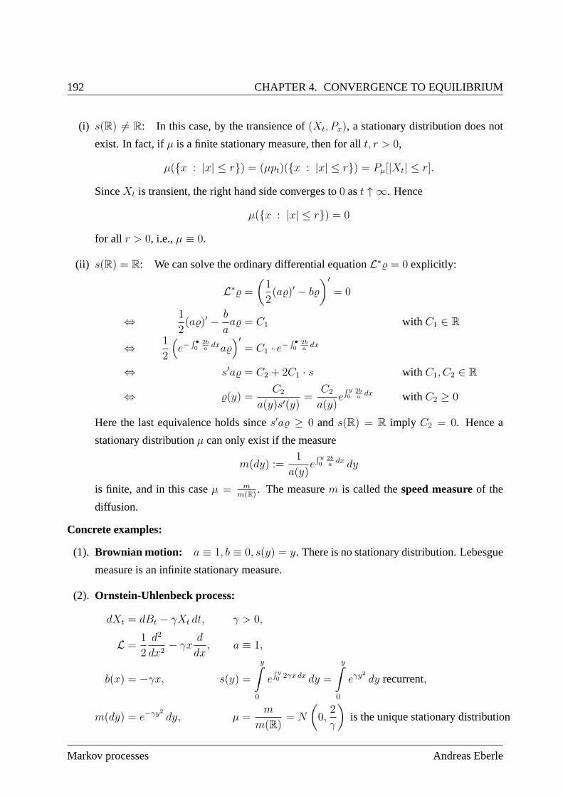
192 CHAPTER 4. CONVERGENCE TO EQUILIBRIUM
(i) s(R) 6= R: In this case, by the transience of(Xt, Px), a stationary distribution does not
exist. In fact, ifµ is a finite stationary measure, then for allt, r > 0,
µ(x : |x| ≤ r) = (µpt)(x : |x| ≤ r) = Pµ[|Xt| ≤ r].
SinceXt is transient, the right hand side converges to0 ast ↑ ∞. Hence
µ(x : |x| ≤ r) = 0
for all r > 0, i.e.,µ ≡ 0.
(ii) s(R) = R: We can solve the ordinary differential equationL∗ = 0 explicitly:
L∗ =
(1
2(a)′ − b
)′= 0
⇔ 1
2(a)′ − b
aa = C1 with C1 ∈ R
⇔ 1
2
(e−´ •0
2ba
dxa)′
= C1 · e−´ •0
2ba
dx
⇔ s′a = C2 + 2C1 · s with C1, C2 ∈ R
⇔ (y) =C2
a(y)s′(y)=
C2
a(y)e´ y0
2ba
dx with C2 ≥ 0
Here the last equivalence holds sinces′a ≥ 0 ands(R) = R imply C2 = 0. Hence a
stationary distributionµ can only exist if the measure
m(dy) :=1
a(y)e´ y0
2ba
dx dy
is finite, and in this caseµ = mm(R)
. The measurem is called thespeed measureof the
diffusion.
Concrete examples:
(1). Brownian motion: a ≡ 1, b ≡ 0, s(y) = y. There is no stationary distribution. Lebesgue
measure is an infinite stationary measure.
(2). Ornstein-Uhlenbeck process:
dXt = dBt − γXt dt, γ > 0,
L =1
2
d2
dx2− γx
d
dx, a ≡ 1,
b(x) = −γx, s(y) =
yˆ
0
e´ y0 2γx dx dy =
yˆ
0
eγy2
dy recurrent,
m(dy) = e−γy2 dy, µ =m
m(R)= N
(0,
2
γ
)is the unique stationary distribution
Markov processes Andreas Eberle
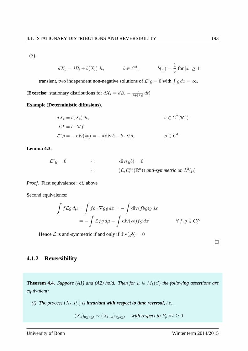
4.1. STATIONARY DISTRIBUTIONS AND REVERSIBILITY 193
(3).
dXt = dBt + b(Xt) dt, b ∈ C2, b(x) =1
xfor |x| ≥ 1
transient, two independent non-negative solutions ofL∗ = 0 with´
dx = ∞.
(Exercise: stationary distributions fordXt = dBt − γ1+|Xt| dt)
Example (Deterministic diffusions).
dXt = b(Xt) dt, b ∈ C2(Rn)
Lf = b · ∇fL∗ = − div(b) = − div b− b · ∇, ∈ C1
Lemma 4.3.
L∗ = 0 ⇔ div(b) = 0
⇔ (L, C∞0 (Rn)) anti-symmetric onL2(µ)
Proof. First equivalence: cf. above
Second equivalence:ˆ
fLg dµ =
ˆ
fb · ∇g dx = −ˆ
div(fb)g dx
= −ˆ
Lfg dµ−ˆ
div(b)fg dx ∀ f, g ∈ C∞0
HenceL is anti-symmetric if and only ifdiv(b) = 0
4.1.2 Reversibility
Theorem 4.4. Suppose (A1) and (A2) hold. Then forµ ∈ M1(S) the following assertions are
equivalent:
(i) The process(Xt, Pµ) is invariant with respect to time reversal, i.e.,
(Xs)0≤s≤t ∼ (Xt−s)0≤s≤t with respect toPµ ∀ t ≥ 0
University of Bonn Winter term 2014/2015
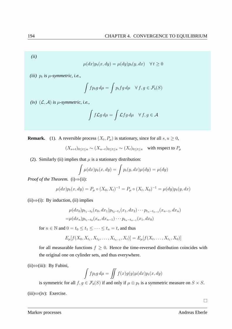
194 CHAPTER 4. CONVERGENCE TO EQUILIBRIUM
(ii)
µ(dx)pt(x, dy) = µ(dy)pt(y, dx) ∀ t ≥ 0
(iii) pt is µ-symmetric, i.e.,ˆ
fptg dµ =
ˆ
ptfg dµ ∀ f, g ∈ Fb(S)
(iv) (L,A) is µ-symmetric, i.e.,ˆ
fLg dµ =
ˆ
Lfg dµ ∀ f, g ∈ A
Remark. (1). A reversible process(Xt, Pµ) is stationary, since for alls, u ≥ 0,
(Xs+t)0≤t≤u ∼ (Xu−t)0≤t≤u ∼ (Xt)0≤t≤u with respect toPµ
(2). Similarly (ii) implies thatµ is a stationary distribution:ˆ
µ(dx)pt(x, dy) =
ˆ
pt(y, dx)µ(dy) = µ(dy)
Proof of the Theorem.(i)⇒(ii):
µ(dx)pt(x, dy) = Pµ (X0, Xt)−1 = Pµ (Xt, X0)
−1 = µ(dy)pt(y, dx)
(ii)⇒(i): By induction, (ii) implies
µ(dx0)pt1−t0(x0, dx1)pt2−t1(x1, dx2) · · · ptn−tn−1(xn−1, dxn)
=µ(dxn)pt1−t0(xn, dxn−1) · · · ptn−tn−1(x1, dx0)
for n ∈ N and0 = t0 ≤ t1 ≤ · · · ≤ tn = t, and thus
Eµ[f(X0, Xt1 , Xt2 , . . . , Xtn−1 , Xt)] = Eµ[f(Xt, . . . , Xt1 , X0)]
for all measurable functionsf ≥ 0. Hence the time-reversed distribution coincides with
the original one on cylinder sets, and thus everywhere.
(ii)⇔(iii): By Fubini,ˆ
fptg dµ =
¨
f(x)g(y)µ(dx)pt(x, dy)
is symmetric for allf, g ∈ Fb(S) if and only if µ⊗ pt is a symmetric measure onS × S.
(iii)⇔(iv): Exercise.
Markov processes Andreas Eberle
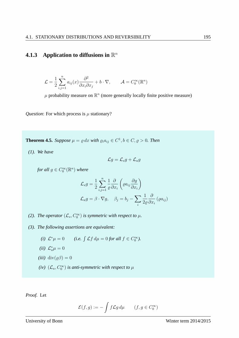
4.1. STATIONARY DISTRIBUTIONS AND REVERSIBILITY 195
4.1.3 Application to diffusions inRn
L =1
2
n∑
i,j=1
aij(x)∂2
∂xi∂xj+ b · ∇, A = C∞
0 (Rn)
µ probability measure onRn (more generally locally finite positive measure)
Question: For which process isµ stationary?
Theorem 4.5.Supposeµ = dx with iaij ∈ C1, b ∈ C, > 0. Then
(1). We have
Lg = Lsg + Lag
for all g ∈ C∞0 (Rn) where
Lsg =1
2
n∑
i,j=1
1
∂
∂xi
(aij
∂g
∂xi
)
Lag = β · ∇g, βj = bj −∑
i
1
2
∂
∂xi(aij)
(2). The operator(Ls, C∞0 ) is symmetric with respect toµ.
(3). The following assertions are equivalent:
(i) L∗µ = 0 (i.e.´
Lf dµ = 0 for all f ∈ C∞0 ).
(ii) L∗aµ = 0
(iii) div(β) = 0
(iv) (La, C∞0 ) is anti-symmetric with respect toµ
Proof. Let
E(f, g) := −ˆ
fLg dµ (f, g ∈ C∞0 )
University of Bonn Winter term 2014/2015
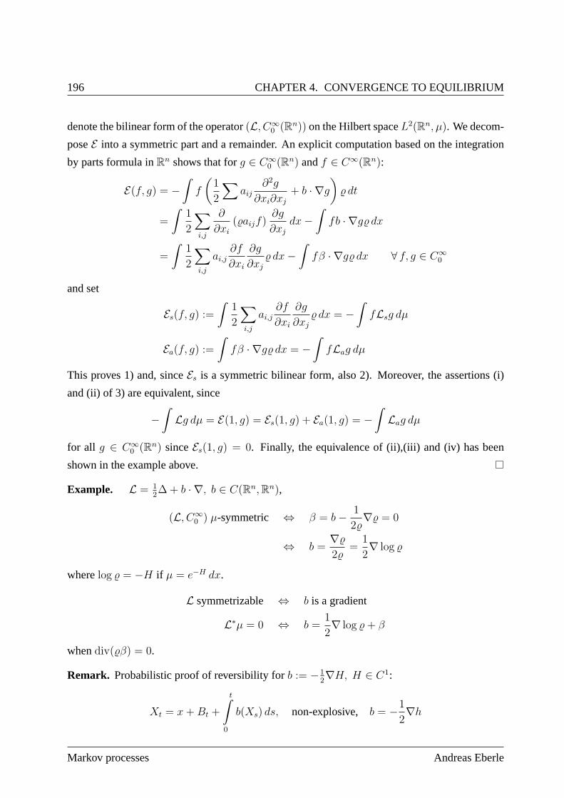
196 CHAPTER 4. CONVERGENCE TO EQUILIBRIUM
denote the bilinear form of the operator(L, C∞0 (Rn)) on the Hilbert spaceL2(Rn, µ). We decom-
poseE into a symmetric part and a remainder. An explicit computation based on the integration
by parts formula inRn shows that forg ∈ C∞0 (Rn) andf ∈ C∞(Rn):
E(f, g) = −ˆ
f
(1
2
∑aij
∂2g
∂xi∂xj+ b · ∇g
) dt
=
ˆ
1
2
∑
i,j
∂
∂xi(aijf)
∂g
∂xjdx−
ˆ
fb · ∇g dx
=
ˆ
1
2
∑
i,j
ai,j∂f
∂xi
∂g
∂xj dx−
ˆ
fβ · ∇g dx ∀ f, g ∈ C∞0
and set
Es(f, g) :=ˆ
1
2
∑
i,j
ai,j∂f
∂xi
∂g
∂xj dx = −
ˆ
fLsg dµ
Ea(f, g) :=ˆ
fβ · ∇g dx = −ˆ
fLag dµ
This proves 1) and, sinceEs is a symmetric bilinear form, also 2). Moreover, the assertions (i)
and (ii) of 3) are equivalent, since
−ˆ
Lg dµ = E(1, g) = Es(1, g) + Ea(1, g) = −ˆ
Lag dµ
for all g ∈ C∞0 (Rn) sinceEs(1, g) = 0. Finally, the equivalence of (ii),(iii) and (iv) has been
shown in the example above.
Example. L = 12∆+ b · ∇, b ∈ C(Rn,Rn),
(L, C∞0 ) µ-symmetric ⇔ β = b− 1
2∇ = 0
⇔ b =∇2
=1
2∇ log
wherelog = −H if µ = e−H dx.
L symmetrizable ⇔ b is a gradient
L∗µ = 0 ⇔ b =1
2∇ log + β
whendiv(β) = 0.
Remark. Probabilistic proof of reversibility forb := −12∇H, H ∈ C1:
Xt = x+Bt +
tˆ
0
b(Xs) ds, non-explosive, b = −1
2∇h
Markov processes Andreas Eberle
4.2. POINCARÉ INEQUALITIES AND CONVERGENCE TO EQUILIBRIUM 197
HencePµ X−10:T ≪ P BM
λ with density
exp
−1
2H(B0)−
1
2H(BT )−
T
0
(1
8|∇H|2 − 1
4∆H
)(Bs) ds
which shows that(Xt, Pµ) is reversible.
4.2 Poincaré inequalities and convergence to equilibrium
Suppose now thatµ is a stationary distribution for(pt)t≥0. Thenpt is a contraction onLp(S, µ)
for all p ∈ [1,∞] sinceˆ
|ptf |p dµ ≤ˆ
pt|f |p dµ =
ˆ
|f |p dµ ∀ f ∈ Fb(S)
by Jensen’s inequality and the stationarity ofµ. As before, we assume that we are given a Markov
process with transition semigroup(pt)t≥0 solving the martingale problem for the operator(L,A).
The assumptions onA0 andA can be relaxed in the following way:
(A0) as above
(A1’) f, Lf ∈ Lp(S, µ) for all 1 ≤ p <∞
(A2’) A0 is dense inA with respect to theLp(S, µ) norms,1 ≤ p < ∞, andptf ∈ A for all
f ∈ A0
In addition, we assume for simplicity
(A3) 1 ∈ A
Remark. Condition (A0) implies thatA, and henceA0, is dense inLp(S, µ) for all p ∈ [1,∞).
In fact, if g ∈ Lq(S, µ), 1q+ 1
q= 1, with
´
fg dµ = 0 for all f ∈ A, theng dµ = 0 by (A0) and
henceg = 0 µ-a.e. Similarly as above, the conditions (A0), (A1’) and (A2’) imply that (pt)t≥0
induces aC0 semigroup onLp(S, µ) for all p ∈ [1,∞), and the generator(L(p),Dom(L(p)))
extends(L,A), i.e.,
A ⊆ Dom(L(p)) and L(p)f = Lf µ-a.e. for allf ∈ A
In particular, the Kolmogorov forward equation
d
dtptf = ptLf ∀ f ∈ A
and the backward equationd
dtptf = Lptf ∀ f ∈ A0
hold with the derivative taken in the Banach spaceLp(S, µ).
University of Bonn Winter term 2014/2015
198 CHAPTER 4. CONVERGENCE TO EQUILIBRIUM
4.2.1 Decay of variances and correlations
We first restrict ourselves to the casep = 2. Forf, g ∈ L2(S, µ) let
(f, g)µ =
ˆ
fg dµ
denote theL2 inner product.
Definition. The bilinear form
E(f, g) := −(f,Lg)µ = − d
dt(f, ptg)µ
∣∣∣t=0,
f, g ∈ A, is called theDirichlet form associated to(L,A) onL2(µ).
Es(f, g) :=1
2(E(f, g) + E(g, f))
is thesymmetrized Dirichlet form.
Remark. More generally,E(f, g) is defined for allf ∈ L2(S, µ) andg ∈ Dom(L(2)) by
E(f, g) = −(f, L(2)g)µ = − d
dt(f, ptg)µ
∣∣∣t=0
Theorem 4.6.For all f ∈ A0 andt ≥ 0
d
dtVarµ(ptf) =
d
dt
ˆ
(ptf)2 dµ = −2E(ptf, ptf) = −2Es(ptf, ptf)
Remark. (1). In particular,
E(f, f) = −1
2
ˆ
(ptf)2 dµ = −1
2
d
dtVarµ(ptf)
∣∣∣t=0,
infinitesimal change of variance
(2). The assertion extends to allf ∈ Dom(L(2)) if the Dirichlet form is defined with respect to
theL2 generator. In the symmetric case the assertion even holds for all f ∈ L2(S, µ).
Proof. By the backward equation,
d
dt
ˆ
(ptf)2 dµ = 2
ˆ
ptLptf dµ = −2E(ptf, ptf) = −2Es(ptf, ptf)
Markov processes Andreas Eberle
4.2. POINCARÉ INEQUALITIES AND CONVERGENCE TO EQUILIBRIUM 199
Moreover, sinceˆ
ptf dµ =
ˆ
f d(µpt) =
ˆ
f dµ
is constant,
d
dtVarµ(ptf) =
d
dt
ˆ
(ptf)2 dµ
Remark. (1). In particular,
E(f, f) = −1
2
d
dt
ˆ
(ptf)2 dµ
∣∣∣t=0
= −1
2
d
dtVarµ(ptf)
Es(f, g) =1
4(Es(f + g, f + g) + Es(f − g, f − g)) = −1
2
d
dtCovµ(ptf, ptg)
Dirichlet form = infinitesimal change of (co)variance.
(2). Sincept is a contraction onL2(µ), the operator(L,A) is negative-definite, and the bilinear
form (E ,A) is positive definite:
(−f,Lf)µ = E(f, f) = −1
2limt↓0
(ˆ
(ptf)2 dµ−
ˆ
f 2 dµ
)≥ 0
Corollary 4.7 (Decay of variance). For λ > 0 the following assertions are equivalent:
(i) Poincaré inequality:
Varµ(f) ≤1
λE(s)(f, f) ∀ f ∈ A
(ii) Exponential decay of variance:
Varµ(ptf) ≤ e−2λt Varµ(f) ∀ f ∈ L2(S, µ) (4.2.1)
(iii) Spectral gap:
Reα ≥ λ ∀α ∈ spec
(−L(2)
∣∣∣span1⊥
)
Remark. Optimizing overλ, the corollary says that (4.2.1) holds with
λ := inff∈A
E(f, f)Varµ(f)
= inff∈A
f⊥1 in L2(µ)
(f,−Lf)µ(f, f)µ
University of Bonn Winter term 2014/2015
200 CHAPTER 4. CONVERGENCE TO EQUILIBRIUM
Proof. (i) ⇒ (ii)
E(f, f) ≥ λ · Varµ(f) ∀ f ∈ A
By the theorem above,
d
dtVarµ(ptf) = −2E(ptf, ptf) ≤ −2λVarµ(ptf)
for all t ≥ 0, f ∈ A0. Hence
Varµ(ptf) ≤ e−2λt Varµ(p0f) = e−2λt Varµ(f)
for all f ∈ A0. Since the right hand side is continuous with respect to theL2(µ) norm, and
A0 is dense inL2(µ) by (A0) and (A2), the inequality extends to allf ∈ L2(µ).
(ii) ⇒ (iii) Forf ∈ Dom(L(2)),
d
dtVarµ(ptf)
∣∣∣t=0
= −2E(f, f).
Hence if (4.2.1) holds then
Varµ(ptf) ≤ e−2λt Varµ(f) ∀ t ≥ 0
which is equivalent to
Varµ(f)− 2tE(f, f) + o(t) ≤ Varµ(f)− 2λtVarµ(f) + o(t) ∀ t ≥ 0
Hence
E(f, f) ≥ λVarµ(f)
and thus
−(L(2)f, f)µ ≥ λ
ˆ
f 2 dµ for f⊥1
which is equivalent to (iii).
(iii) ⇒ (i) Follows by the equivalence above.
Remark. Since(L,A) is negative definite,λ ≥ 0. In order to obtain exponential decay, however,
we needλ > 0, which is not always the case.
Markov processes Andreas Eberle
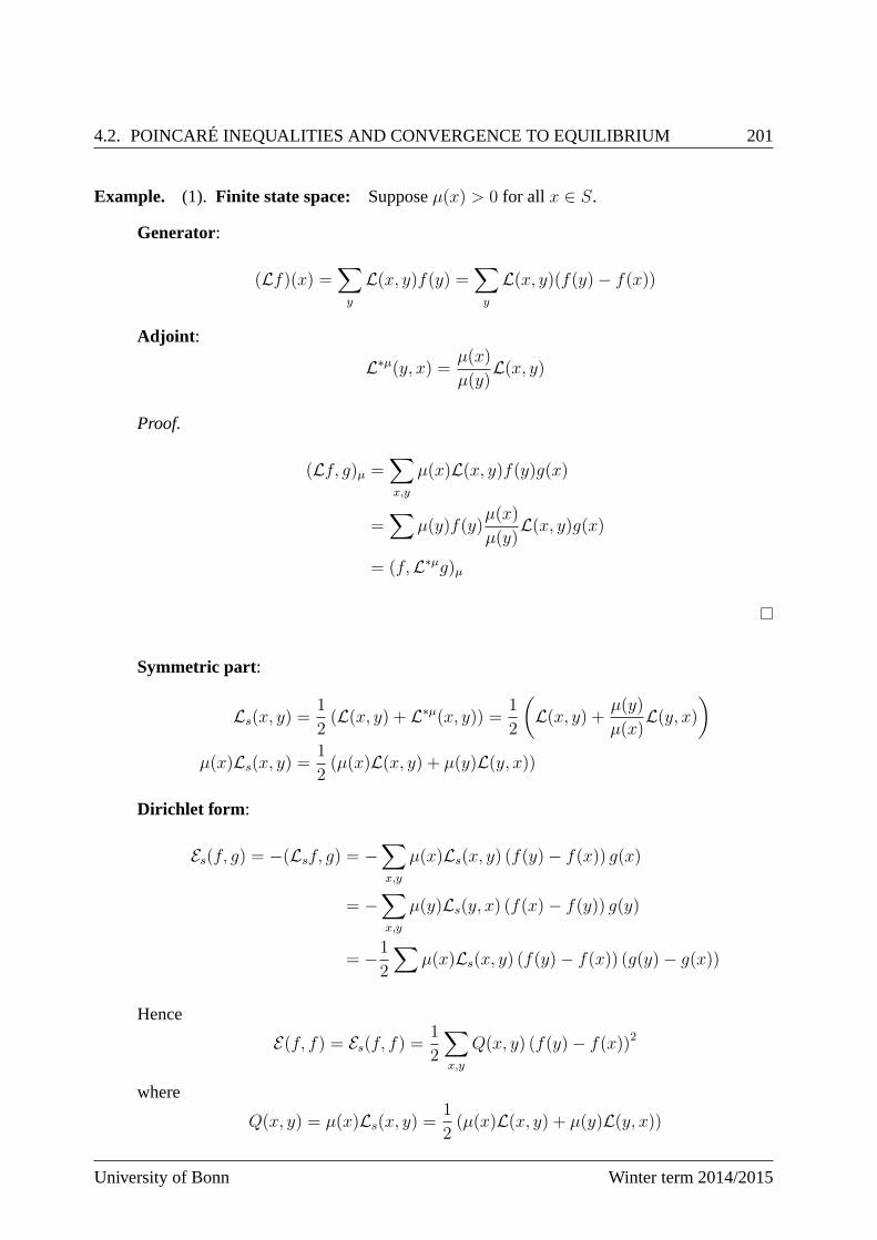
4.2. POINCARÉ INEQUALITIES AND CONVERGENCE TO EQUILIBRIUM 201
Example. (1). Finite state space: Supposeµ(x) > 0 for all x ∈ S.
Generator:
(Lf)(x) =∑
y
L(x, y)f(y) =∑
y
L(x, y)(f(y)− f(x))
Adjoint :
L∗µ(y, x) =µ(x)
µ(y)L(x, y)
Proof.
(Lf, g)µ =∑
x,y
µ(x)L(x, y)f(y)g(x)
=∑
µ(y)f(y)µ(x)
µ(y)L(x, y)g(x)
= (f,L∗µg)µ
Symmetric part:
Ls(x, y) =1
2(L(x, y) + L∗µ(x, y)) =
1
2
(L(x, y) + µ(y)
µ(x)L(y, x)
)
µ(x)Ls(x, y) =1
2(µ(x)L(x, y) + µ(y)L(y, x))
Dirichlet form :
Es(f, g) = −(Lsf, g) = −∑
x,y
µ(x)Ls(x, y) (f(y)− f(x)) g(x)
= −∑
x,y
µ(y)Ls(y, x) (f(x)− f(y)) g(y)
= −1
2
∑µ(x)Ls(x, y) (f(y)− f(x)) (g(y)− g(x))
Hence
E(f, f) = Es(f, f) =1
2
∑
x,y
Q(x, y) (f(y)− f(x))2
where
Q(x, y) = µ(x)Ls(x, y) =1
2(µ(x)L(x, y) + µ(y)L(y, x))
University of Bonn Winter term 2014/2015
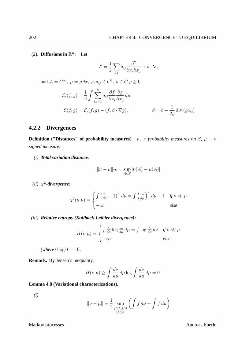
202 CHAPTER 4. CONVERGENCE TO EQUILIBRIUM
(2). Diffusions in Rn: Let
L =1
2
∑
i,j
aij∂2
∂xi∂xj+ b · ∇,
andA = C∞0 , µ = dx, , aij ∈ C1, b ∈ C ≥ 0,
Es(f, g) =1
2
ˆ n∑
i,j=1
aij∂f
∂xi
∂g
∂xjdµ
E(f, g) = Es(f, g)− (f, β · ∇g), β = b− 1
2div (aij)
4.2.2 Divergences
Definition ("Distances" of probability measures). µ, ν probability measures onS, µ − ν
signed measure.
(i) Total variation distance:
‖ν − µ‖TV = supA∈S
|ν(A)− µ(A)|
(ii) χ2-divergence:
χ2(µ|ν) =
´ (dµdν
− 1)2dµ =
´
(dνdµ
)2dµ− 1 if ν ≪ µ
+∞ else
(iii) Relative entropy (Kullback-Leibler divergence):
H(ν|µ) =
´
dνdµ
log dνdµdµ =
´
log dνdµdν if ν ≪ µ
+∞ else
(where0 log 0 := 0).
Remark. By Jensen’s inequality,
H(ν|µ) ≥ˆ
dν
dµdµ log
ˆ
dν
dµdµ = 0
Lemma 4.8(Variational characterizations).
(i)
‖ν − µ‖ =1
2sup
f∈Fb(S)|f |≤1
(ˆ
f dν −ˆ
f dµ
)
Markov processes Andreas Eberle
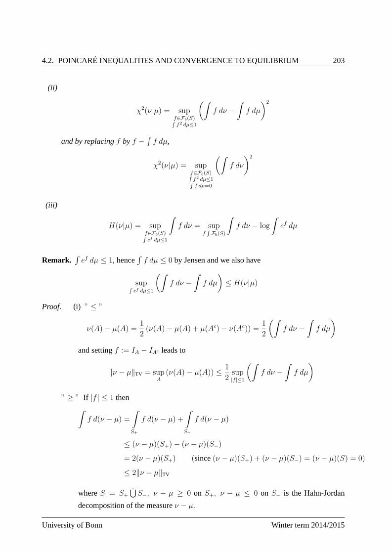
4.2. POINCARÉ INEQUALITIES AND CONVERGENCE TO EQUILIBRIUM 203
(ii)
χ2(ν|µ) = supf∈Fb(S)´
f2 dµ≤1
(ˆ
f dν −ˆ
f dµ
)2
and by replacingf byf −´
f dµ,
χ2(ν|µ) = supf∈Fb(S)´
f2 dµ≤1´
f dµ=0
(ˆ
f dν
)2
(iii)
H(ν|µ) = supf∈Fb(S)´
ef dµ≤1
ˆ
f dν = supf´
Fb(S)
ˆ
f dν − log
ˆ
ef dµ
Remark.´
ef dµ ≤ 1, hence´
f dµ ≤ 0 by Jensen and we also have
sup´
ef dµ≤1
(ˆ
f dν −ˆ
f dµ
)≤ H(ν|µ)
Proof. (i) ” ≤ ”
ν(A)− µ(A) =1
2(ν(A)− µ(A) + µ(Ac)− ν(Ac)) =
1
2
(ˆ
f dν −ˆ
f dµ
)
and settingf := IA − IAc leads to
‖ν − µ‖TV = supA
(ν(A)− µ(A)) ≤ 1
2sup|f |≤1
(ˆ
f dν −ˆ
f dµ
)
” ≥ ” If |f | ≤ 1 thenˆ
f d(ν − µ) =
ˆ
S+
f d(ν − µ) +
ˆ
S−
f d(ν − µ)
≤ (ν − µ)(S+)− (ν − µ)(S−)
= 2(ν − µ)(S+) (since(ν − µ)(S+) + (ν − µ)(S−) = (ν − µ)(S) = 0)
≤ 2‖ν − µ‖TV
whereS = S+
⋃S−, ν − µ ≥ 0 on S+, ν − µ ≤ 0 on S− is the Hahn-Jordan
decomposition of the measureν − µ.
University of Bonn Winter term 2014/2015
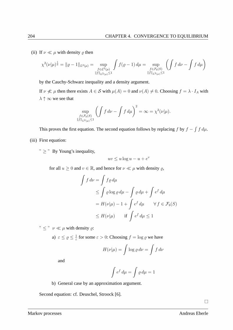
204 CHAPTER 4. CONVERGENCE TO EQUILIBRIUM
(ii) If ν ≪ µ with density then
χ2(ν|µ) 12 = ‖− 1‖L2(µ) = sup
f∈L2(µ)‖f‖L2(µ)≤1
ˆ
f(− 1) dµ = supf∈Fb(S)
‖f‖L2(µ)≤1
(ˆ
f dν −ˆ
f dµ
)
by the Cauchy-Schwarz inequality and a density argument.
If ν 6≪ µ then there existsA ∈ S with µ(A) = 0 andν(A) 6= 0. Choosingf = λ · IA with
λ ↑ ∞ we see that
supf∈Fb(S)
‖f‖L2(µ)≤1
(ˆ
f dν −ˆ
f dµ
)2
= ∞ = χ2(ν|µ).
This proves the first equation. The second equation follows by replacingf by f −´
f dµ.
(iii) First equation:
” ≥ ” By Young’s inequality,
uv ≤ u log u− u+ ev
for all u ≥ 0 andv ∈ R, and hence forν ≪ µ with density,ˆ
f dν =
ˆ
f dµ
≤ˆ
log dµ−ˆ
dµ+
ˆ
ef dµ
= H(ν|µ)− 1 +
ˆ
ef dµ ∀ f ∈ Fb(S)
≤ H(ν|µ) ifˆ
ef dµ ≤ 1
” ≤ ” ν ≪ µ with density:
a) ε ≤ ≤ 1ε
for someε > 0: Choosingf = log we have
H(ν|µ) =ˆ
log dν =
ˆ
f dν
andˆ
ef dµ =
ˆ
dµ = 1
b) General case by an approximation argument.
Second equation: cf. Deuschel, Stroock [6].
Markov processes Andreas Eberle
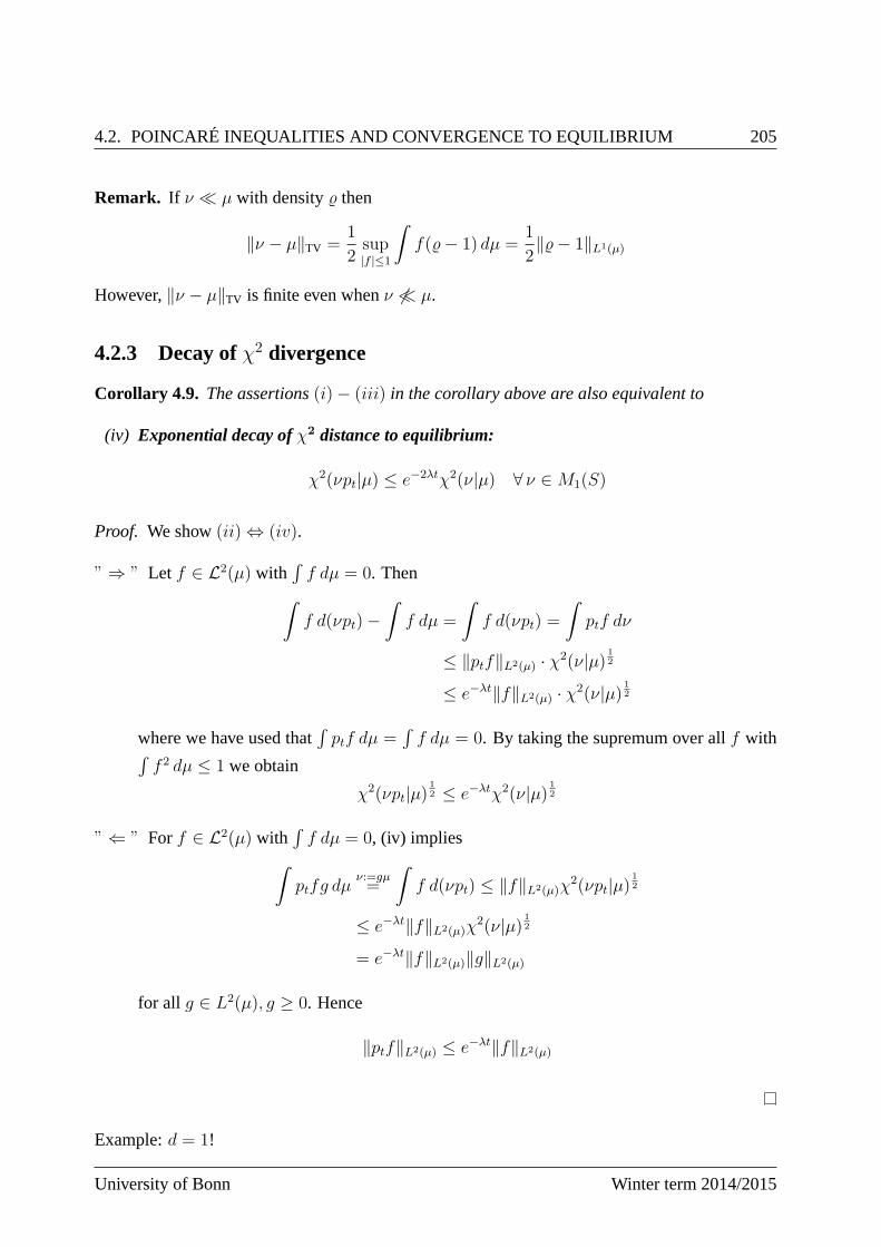
4.2. POINCARÉ INEQUALITIES AND CONVERGENCE TO EQUILIBRIUM 205
Remark. If ν ≪ µ with density then
‖ν − µ‖TV =1
2sup|f |≤1
ˆ
f(− 1) dµ =1
2‖− 1‖L1(µ)
However,‖ν − µ‖TV is finite even whenν 6≪ µ.
4.2.3 Decay ofχ2 divergence
Corollary 4.9. The assertions(i)− (iii) in the corollary above are also equivalent to
(iv) Exponential decay ofχ2 distance to equilibrium:
χ2(νpt|µ) ≤ e−2λtχ2(ν|µ) ∀ ν ∈M1(S)
Proof. We show(ii) ⇔ (iv).
” ⇒ ” Let f ∈ L2(µ) with´
f dµ = 0. Thenˆ
f d(νpt)−ˆ
f dµ =
ˆ
f d(νpt) =
ˆ
ptf dν
≤ ‖ptf‖L2(µ) · χ2(ν|µ) 12
≤ e−λt‖f‖L2(µ) · χ2(ν|µ) 12
where we have used that´
ptf dµ =´
f dµ = 0. By taking the supremum over allf with´
f 2 dµ ≤ 1 we obtain
χ2(νpt|µ)12 ≤ e−λtχ2(ν|µ) 1
2
” ⇐ ” Forf ∈ L2(µ) with´
f dµ = 0, (iv) impliesˆ
ptfg dµν:=gµ=
ˆ
f d(νpt) ≤ ‖f‖L2(µ)χ2(νpt|µ)
12
≤ e−λt‖f‖L2(µ)χ2(ν|µ) 1
2
= e−λt‖f‖L2(µ)‖g‖L2(µ)
for all g ∈ L2(µ), g ≥ 0. Hence
‖ptf‖L2(µ) ≤ e−λt‖f‖L2(µ)
Example:d = 1!
University of Bonn Winter term 2014/2015
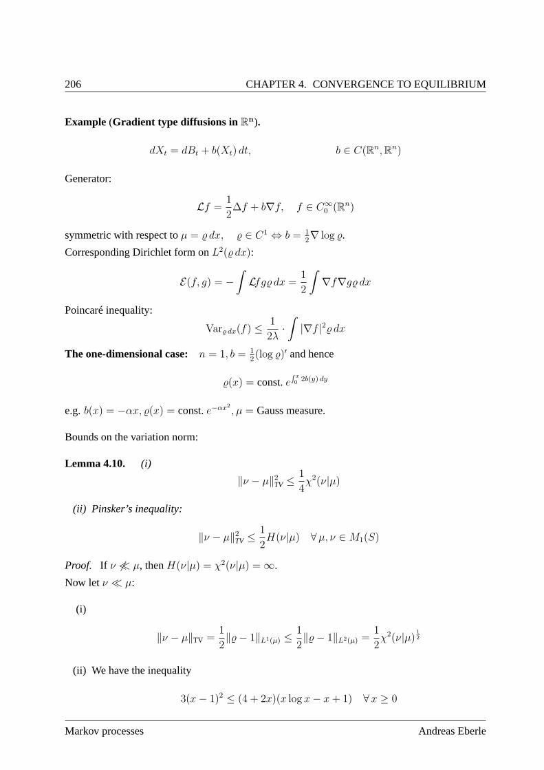
206 CHAPTER 4. CONVERGENCE TO EQUILIBRIUM
Example (Gradient type diffusions in Rn).
dXt = dBt + b(Xt) dt, b ∈ C(Rn,Rn)
Generator:
Lf =1
2∆f + b∇f, f ∈ C∞
0 (Rn)
symmetric with respect toµ = dx, ∈ C1 ⇔ b = 12∇ log .
Corresponding Dirichlet form onL2( dx):
E(f, g) = −ˆ
Lfg dx =1
2
ˆ
∇f∇g dx
Poincaré inequality:
Var dx(f) ≤1
2λ·ˆ
|∇f |2 dx
The one-dimensional case: n = 1, b = 12(log )′ and hence
(x) = const.e´ x0 2b(y) dy
e.g.b(x) = −αx, (x) = const.e−αx2, µ = Gauss measure.
Bounds on the variation norm:
Lemma 4.10. (i)
‖ν − µ‖2TV ≤ 1
4χ2(ν|µ)
(ii) Pinsker’s inequality:
‖ν − µ‖2TV ≤ 1
2H(ν|µ) ∀µ, ν ∈M1(S)
Proof. If ν 6≪ µ, thenH(ν|µ) = χ2(ν|µ) = ∞.
Now letν ≪ µ:
(i)
‖ν − µ‖TV =1
2‖− 1‖L1(µ) ≤
1
2‖− 1‖L2(µ) =
1
2χ2(ν|µ) 1
2
(ii) We have the inequality
3(x− 1)2 ≤ (4 + 2x)(x log x− x+ 1) ∀ x ≥ 0
Markov processes Andreas Eberle
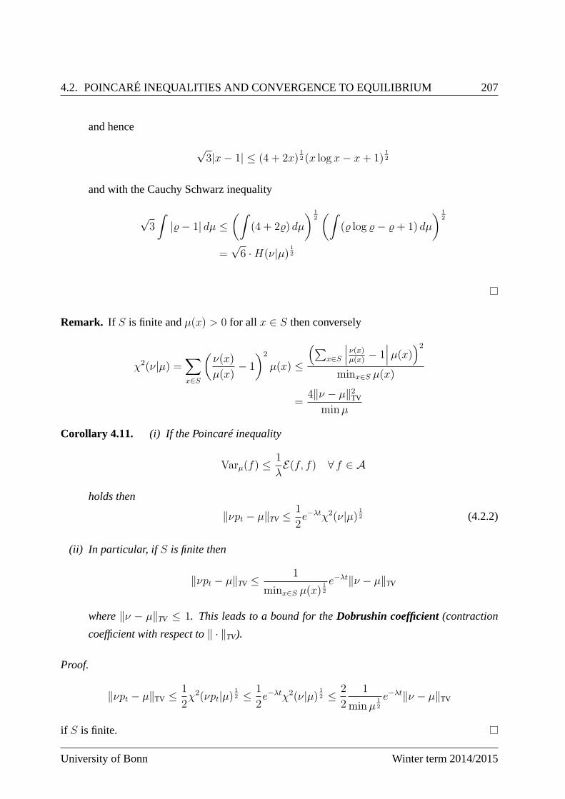
4.2. POINCARÉ INEQUALITIES AND CONVERGENCE TO EQUILIBRIUM 207
and hence
√3|x− 1| ≤ (4 + 2x)
12 (x log x− x+ 1)
12
and with the Cauchy Schwarz inequality
√3
ˆ
|− 1| dµ ≤(ˆ
(4 + 2) dµ
) 12(ˆ
( log − + 1) dµ
) 12
=√6 ·H(ν|µ) 1
2
Remark. If S is finite andµ(x) > 0 for all x ∈ S then conversely
χ2(ν|µ) =∑
x∈S
(ν(x)
µ(x)− 1
)2
µ(x) ≤
(∑x∈S
∣∣∣ ν(x)µ(x)− 1∣∣∣µ(x)
)2
minx∈S µ(x)
=4‖ν − µ‖2TV
minµ
Corollary 4.11. (i) If the Poincaré inequality
Varµ(f) ≤1
λE(f, f) ∀ f ∈ A
holds then
‖νpt − µ‖TV ≤ 1
2e−λtχ2(ν|µ) 1
2 (4.2.2)
(ii) In particular, if S is finite then
‖νpt − µ‖TV ≤ 1
minx∈S µ(x)12
e−λt‖ν − µ‖TV
where‖ν − µ‖TV ≤ 1. This leads to a bound for theDobrushin coefficient(contraction
coefficient with respect to‖ · ‖TV).
Proof.
‖νpt − µ‖TV ≤ 1
2χ2(νpt|µ)
12 ≤ 1
2e−λtχ2(ν|µ) 1
2 ≤ 2
2
1
minµ12
e−λt‖ν − µ‖TV
if S is finite.
University of Bonn Winter term 2014/2015
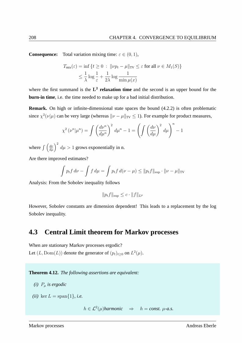
208 CHAPTER 4. CONVERGENCE TO EQUILIBRIUM
Consequence: Total variation mixing time:ε ∈ (0, 1),
Tmix(ε) = inf t ≥ 0 : ‖νpt − µ‖TV ≤ ε for all ν ∈M1(S)
≤ 1
λlog
1
ε+
1
2λlog
1
minµ(x)
where the first summand is theL2 relaxation time and the second is an upper bound for the
burn-in time , i.e. the time needed to make up for a bad initial distribution.
Remark. On high or infinite-dimensional state spaces the bound (4.2.2) is often problematic
sinceχ2(ν|µ) can be very large (whereas‖ν − µ‖TV ≤ 1). For example for product measures,
χ2 (νn|µn) =
ˆ(dνn
dµn
)2
dµn − 1 =
(ˆ(dν
dµ
)2
dµ
)n
− 1
where´
(dνdµ
)2dµ > 1 grows exponentially in n.
Are there improved estimates?ˆ
ptf dν −ˆ
f dµ =
ˆ
ptf d(ν − µ) ≤ ‖ptf‖sup · ‖ν − µ‖TV
Analysis: From the Sobolev inequality follows
‖ptf‖sup ≤ c · ‖f‖Lp
However, Sobolev constants are dimension dependent! This leads to a replacement by the log
Sobolev inequality.
4.3 Central Limit theorem for Markov processes
When are stationary Markov processes ergodic?
Let (L,Dom(L)) denote the generator of(pt)t≥0 onL2(µ).
Theorem 4.12.The following assertions are equivalent:
(i) Pµ is ergodic
(ii) kerL = span1, i.e.
h ∈ L2(µ)harmonic ⇒ h = const.µ-a.s.
Markov processes Andreas Eberle
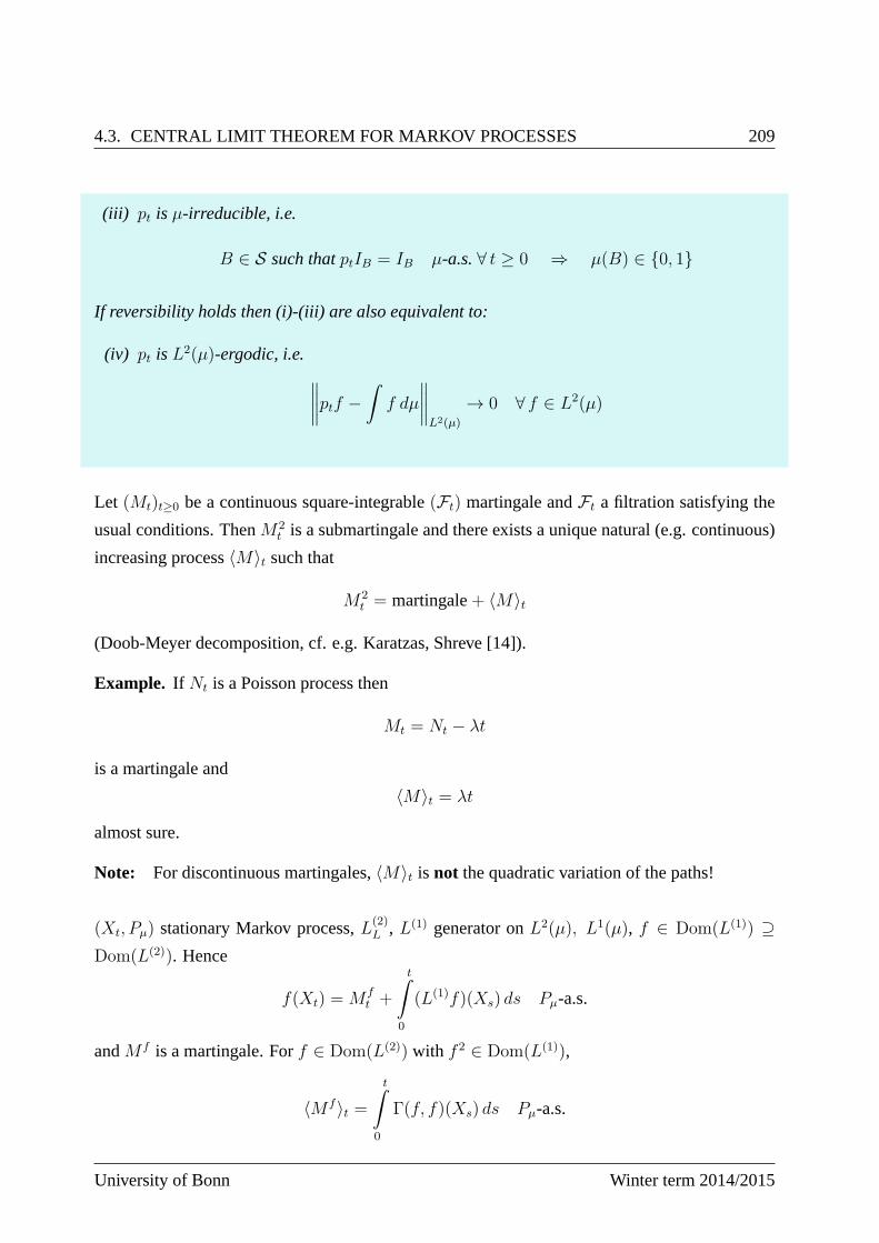
4.3. CENTRAL LIMIT THEOREM FOR MARKOV PROCESSES 209
(iii) pt is µ-irreducible, i.e.
B ∈ S such thatptIB = IB µ-a.s.∀ t ≥ 0 ⇒ µ(B) ∈ 0, 1
If reversibility holds then (i)-(iii) are also equivalent to:
(iv) pt isL2(µ)-ergodic, i.e.∥∥∥∥ptf −
ˆ
f dµ
∥∥∥∥L2(µ)
→ 0 ∀ f ∈ L2(µ)
Let (Mt)t≥0 be a continuous square-integrable(Ft) martingale andFt a filtration satisfying the
usual conditions. ThenM2t is a submartingale and there exists a unique natural (e.g. continuous)
increasing process〈M〉t such that
M2t = martingale+ 〈M〉t
(Doob-Meyer decomposition, cf. e.g. Karatzas, Shreve [14]).
Example. If Nt is a Poisson process then
Mt = Nt − λt
is a martingale and
〈M〉t = λt
almost sure.
Note: For discontinuous martingales,〈M〉t is not the quadratic variation of the paths!
(Xt, Pµ) stationary Markov process,L(2)L , L(1) generator onL2(µ), L1(µ), f ∈ Dom(L(1)) ⊇
Dom(L(2)). Hence
f(Xt) =M ft +
tˆ
0
(L(1)f)(Xs) ds Pµ-a.s.
andM f is a martingale. Forf ∈ Dom(L(2)) with f 2 ∈ Dom(L(1)),
〈M f〉t =tˆ
0
Γ(f, f)(Xs) ds Pµ-a.s.
University of Bonn Winter term 2014/2015
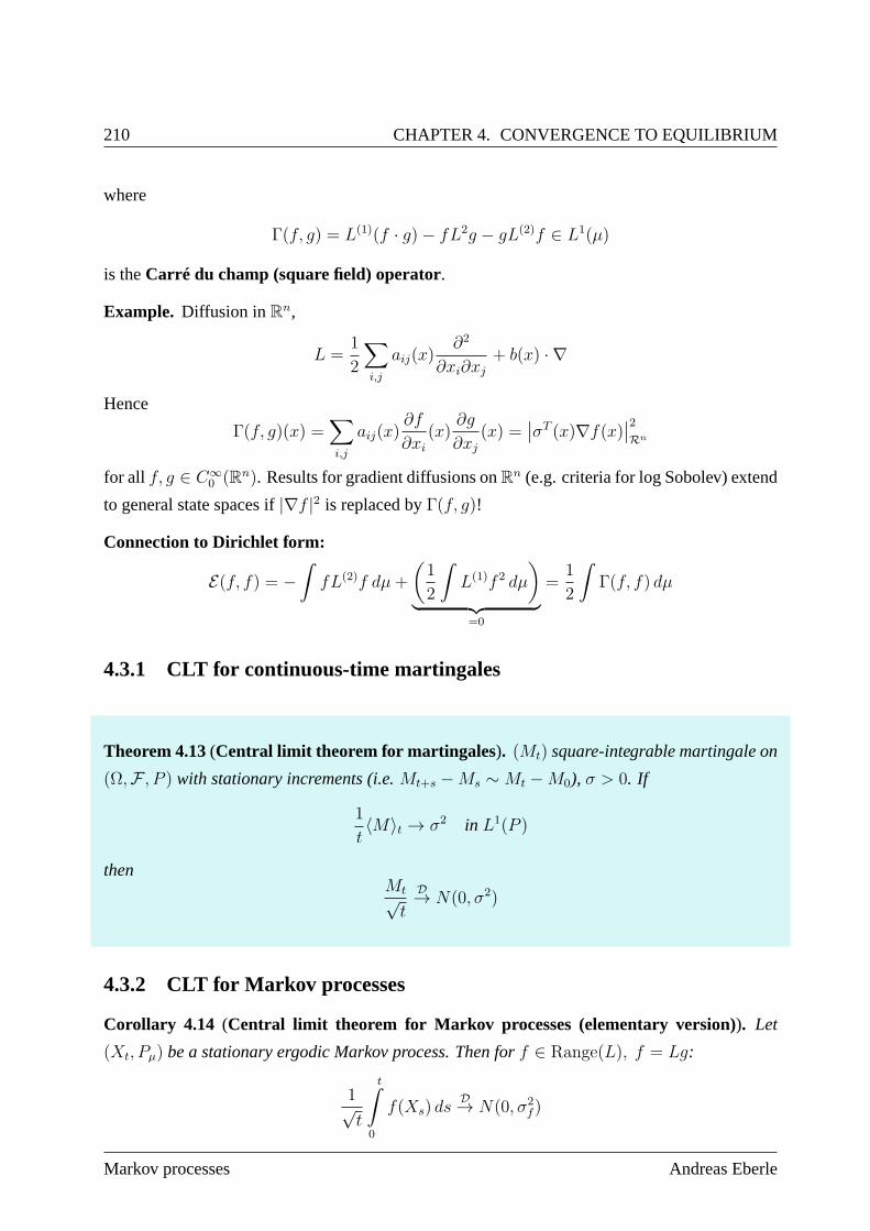
210 CHAPTER 4. CONVERGENCE TO EQUILIBRIUM
where
Γ(f, g) = L(1)(f · g)− fL2g − gL(2)f ∈ L1(µ)
is theCarré du champ (square field) operator.
Example. Diffusion inRn,
L =1
2
∑
i,j
aij(x)∂2
∂xi∂xj+ b(x) · ∇
Hence
Γ(f, g)(x) =∑
i,j
aij(x)∂f
∂xi(x)
∂g
∂xj(x) =
∣∣σT (x)∇f(x)∣∣2Rn
for all f, g ∈ C∞0 (Rn). Results for gradient diffusions onRn (e.g. criteria for log Sobolev) extend
to general state spaces if|∇f |2 is replaced byΓ(f, g)!
Connection to Dirichlet form:
E(f, f) = −ˆ
fL(2)f dµ+
(1
2
ˆ
L(1)f 2 dµ
)
︸ ︷︷ ︸=0
=1
2
ˆ
Γ(f, f) dµ
4.3.1 CLT for continuous-time martingales
Theorem 4.13(Central limit theorem for martingales ). (Mt) square-integrable martingale on
(Ω,F , P ) with stationary increments (i.e.Mt+s −Ms ∼Mt −M0), σ > 0. If
1
t〈M〉t → σ2 in L1(P )
thenMt√t
D→ N(0, σ2)
4.3.2 CLT for Markov processes
Corollary 4.14 (Central limit theorem for Markov processes (elementary version)). Let
(Xt, Pµ) be a stationary ergodic Markov process. Then forf ∈ Range(L), f = Lg:
1√t
tˆ
0
f(Xs) dsD→ N(0, σ2
f )
Markov processes Andreas Eberle
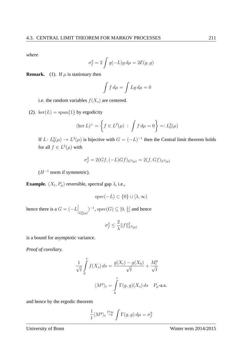
4.3. CENTRAL LIMIT THEOREM FOR MARKOV PROCESSES 211
where
σ2f = 2
ˆ
g(−L)g dµ = 2E(g, g)
Remark. (1). If µ is stationary thenˆ
f dµ =
ˆ
Lg dµ = 0
i.e. the random variablesf(Xs) are centered.
(2). ker(L) = span1 by ergodicity
(kerL)⊥ =
f ∈ L2(µ) :
ˆ
f dµ = 0
=: L2
0(µ)
If L : L20(µ) → L2(µ) is bijective withG = (−L)−1 then the Central limit theorem holds
for all f ∈ L2(µ) with
σ2f = 2(Gf, (−L)Gf)L2(µ) = 2(f,Gf)L2(µ)
(H−1 norm if symmetric).
Example. (Xt, Pµ) reversible, spectral gapλ, i.e.,
spec(−L) ⊂ 0 ∪ [λ,∞)
hence there is aG = (−L∣∣∣L20(µ)
)−1, spec(G) ⊆ [0, 1λ] and hence
σ2f ≤ 2
λ‖f‖2L2(µ)
is a bound for asymptotic variance.
Proof of corollary.
1√t
tˆ
0
f(Xs) ds =g(Xt)− g(X0)√
t+M g
t√t
〈M g〉t =tˆ
0
Γ(g, g)(Xs) ds Pµ-a.s.
and hence by the ergodic theorem
1
t〈M g〉t t↑∞→
ˆ
Γ(g, g) dµ = σ2f
University of Bonn Winter term 2014/2015
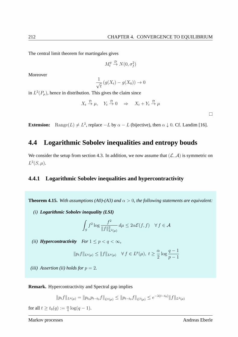
212 CHAPTER 4. CONVERGENCE TO EQUILIBRIUM
The central limit theorem for martingales gives
M gt
D→ N(0, σ2f )
Moreover1√t(g(Xt)− g(X0)) → 0
in L2(Pµ), hence in distribution. This gives the claim since
XtD→ µ, Yt
D→ 0 ⇒ Xt + YtD→ µ
Extension: Range(L) 6= L2, replace−L by α− L (bijective), thenα ↓ 0. Cf. Landim [16].
4.4 Logarithmic Sobolev inequalities and entropy bouds
We consider the setup from section 4.3. In addition, we now assume that(L,A) is symmetric on
L2(S, µ).
4.4.1 Logarithmic Sobolev inequalities and hypercontractivity
Theorem 4.15.With assumptions (A0)-(A3) andα > 0, the following statements are equivalent:
(i) Logarithmic Sobolev inequality (LSI)ˆ
S
f 2 logf 2
‖f‖2L2(µ)
dµ ≤ 2αE(f, f) ∀ f ∈ A
(ii) Hypercontractivity For 1 ≤ p < q <∞,
‖ptf‖Lq(µ) ≤ ‖f‖Lp(µ) ∀ f ∈ Lp(µ), t ≥ α
2log
q − 1
p− 1
(iii) Assertion (ii) holds forp = 2.
Remark. Hypercontractivity and Spectral gap implies
‖ptf‖Lq(µ) = ‖pt0pt−t0f‖Lq(µ) ≤ ‖pt−t0f‖L2(µ) ≤ e−λ(t−t0)‖f‖L2(µ)
for all t ≥ t0(q) :=α4log(q − 1).
Markov processes Andreas Eberle
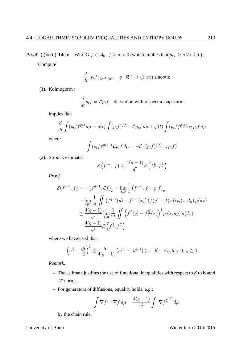
4.4. LOGARITHMIC SOBOLEV INEQUALITIES AND ENTROPY BOUDS 213
Proof. (i)⇒(ii) Idea: WLOG f ∈ A0, f ≥ δ > 0 (which implies thatptf ≥ δ ∀ t ≥ 0).
Compute
d
dt‖ptf‖Lq(t)(µ), q : R+ → (1,∞) smooth:
(1). Kolmogorov:
d
dtptf = Lptf derivation with respect to sup-norm
implies that
d
dt
ˆ
(ptf)q(t) dµ = q(t)
ˆ
(ptf)q(t)−1Lptf dµ+ q′(t)
ˆ
(ptf)q(t) log ptf dµ
whereˆ
(ptf)q(t)−1Lptf dµ = −E
((ptf)
q(t)−1, ptf)
(2). Stroock estimate:
E(f q−1, f
)≥ 4(q − 1)
q2E(f
q2 , f
q2
)
Proof.
E(f q−1, f) = −(f q−1,Lf
)µ= lim
t↓0
1
t
(f q−1, f − ptf
)µ
= limt↓0
1
2t
¨ (f q−1(y)− f q−1(x)
)(f(y)− f(x)) pt(x, dy)µ(dx)
≥ 4(q − 1)
q2limt↓0
1
2t
¨ (f
q2 (y)− f
q
2(x))2pt(x, dy)µ(dx)
=4(q − 1)
q2E(f
q2 , f
q2
)
where we have used that(a
q2 − b
q
2
)2≤ q2
4(q − 1)
(aq−1 − bq−1
)(a− b) ∀ a, b > 0, q ≥ 1
Remark.
– The estimate justifies the use of functional inequalities with respect toE to bound
Lp norms.
– For generators of diffusions, equality holds, e.g.:ˆ
∇f q−1∇f dµ =4(q − 1)
q2
ˆ ∣∣∣∇f q2
∣∣∣2
dµ
by the chain rule.
University of Bonn Winter term 2014/2015
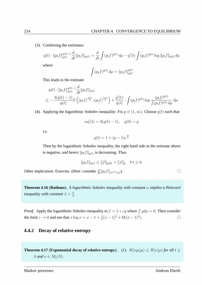
214 CHAPTER 4. CONVERGENCE TO EQUILIBRIUM
(3). Combining the estimates:
q(t) · ‖ptf‖q(t)−1q(t)
d
dt‖ptf‖q(t) =
d
dt
ˆ
(ptf)q(t) dµ− q′(t)
ˆ
(ptf)q(t) log ‖ptf‖q(t) dµ
whereˆ
(ptf)q(t) dµ = ‖ptf‖q(t)q(t)
This leads to the estimate
q(t) · ‖ptf‖q(t)−1q(t)
d
dt‖ptf‖q(t)
≤− 4(q(t)− 1)
q(t)E((ptf)
q(t)2 , (ptf)
q(t)2
)+q′(t)
q(t)·ˆ
(ptf)q(t) log
(ptf)q(t)
´
(ptf)q(t) dµdµ
(4). Applying the logarithmic Sobolev inequality: Fixp ∈ (1,∞). Chooseq(t) such that
αq′(t) = 2(q(t)− 1), q(0) = p
i.e.
q(t) = 1 + (p− 1)e2tα
Then by the logarithmic Sobolev inequality, the right hand side in the estimate above
is negative, and hence‖ptf‖q(t) is decreasing. Thus
‖ptf‖q(t) ≤ ‖f‖q(0) = ‖f‖p ∀ t ≥ 0.
Other implication: Exercise. (Hint: considerddt‖ptf‖Lq(t)(µ)).
Theorem 4.16(Rothaus). A logarithmic Sobolev inequality with constantα implies a Poincaré
inequality with constantλ = 2α.
Proof. Apply the logarithmic Sobolev-inequality tof = 1+εg where´
gdµ = 0. Then consider
the limit ε→ 0 and use thatx log x = x− 1 + 12(x− 1)2 + O(|x− 1|3).
4.4.2 Decay of relative entropy
Theorem 4.17(Exponential decay of relative entropy). (1). H(νpt|µ) ≤ H(ν|µ) for all t ≥0 andν ∈M1(S).
Markov processes Andreas Eberle
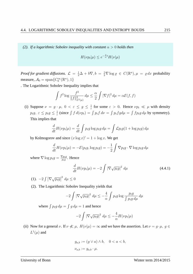
4.4. LOGARITHMIC SOBOLEV INEQUALITIES AND ENTROPY BOUDS 215
(2). If a logarithmic Sobolev inequality with constantα > 0 holds then
H(νpt|µ) ≤ e−2αtH(ν|µ)
Proof for gradient diffusions.L = 12∆ + b∇, b = 1
2∇ log ∈ C(Rn), µ = dx probability
measure,A0 = spanC∞0 (Rn), 1
. The Logarithmic Sobolev Inequality implies thatˆ
f 2 logf 2
‖f‖2L2(µ)
dµ ≤ α
2
ˆ
|∇f |2 dµ = αE(f, f)
(i) Supposeν = g · µ, 0 < ε ≤ g ≤ 1ε
for someε > 0. Henceνpt ≪ µ with density
ptg, ε ≤ ptg ≤ 1ε
(since´
f d(νpt) =´
ptf dν =´
ptfgdµ =´
fptg dµ by symmetry).
This implies that
d
dtH(νpt|µ) =
d
dt
ˆ
ptg log ptg dµ =
ˆ
Lptg(1 + log ptg) dµ
by Kolmogorov and since(x log x)′ = 1 + log x. We get
d
dtH(νpt|µ) = −E(ptg, log ptg) = −1
2
ˆ
∇ptg · ∇ log ptg dµ
where∇ log ptg =∇ptgptg
. Hence
d
dtH(νpt|µ) = −2
ˆ
|∇√ptg|2 dµ (4.4.1)
(1). −2´∣∣∇√
ptg∣∣2 dµ ≤ 0
(2). The Logarithmic Sobolev Inequality yields that
−2
ˆ
|∇√ptg|2 dµ ≤ − 4
α
ˆ
ptg logptg
´
ptg dµdµ
where´
ptg dµ =´
g dµ = 1 and hence
−2
ˆ
|∇√ptg|2 dµ ≤ − 4
αH(νpt|µ)
(ii) Now for a generalν. If ν 6≪ µ, H(ν|µ) = ∞ and we have the assertion. Letν = g ·µ, g ∈L1(µ) and
ga,b := (g ∨ a) ∧ b, 0 < a < b,
νa,b := ga,b · µ.
University of Bonn Winter term 2014/2015
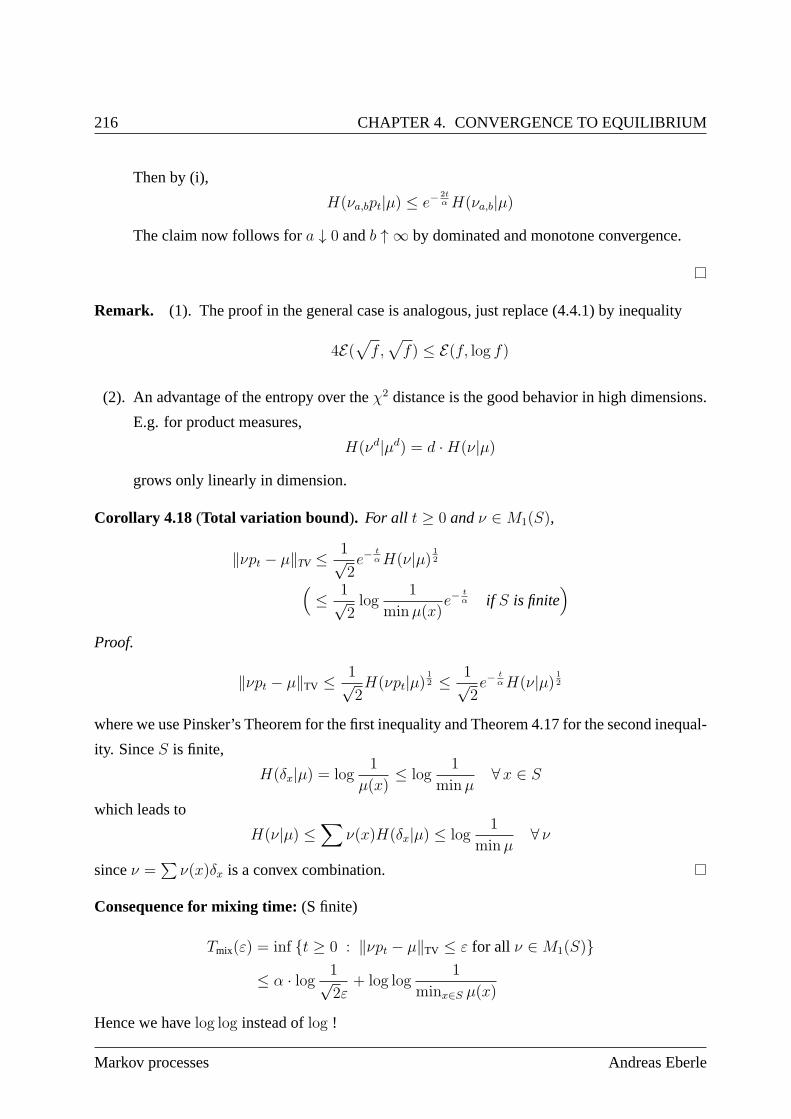
216 CHAPTER 4. CONVERGENCE TO EQUILIBRIUM
Then by (i),
H(νa,bpt|µ) ≤ e−2tαH(νa,b|µ)
The claim now follows fora ↓ 0 andb ↑ ∞ by dominated and monotone convergence.
Remark. (1). The proof in the general case is analogous, just replace(4.4.1) by inequality
4E(√f,√f) ≤ E(f, log f)
(2). An advantage of the entropy over theχ2 distance is the good behavior in high dimensions.
E.g. for product measures,
H(νd|µd) = d ·H(ν|µ)
grows only linearly in dimension.
Corollary 4.18 (Total variation bound ). For all t ≥ 0 andν ∈M1(S),
‖νpt − µ‖TV ≤ 1√2e−
tαH(ν|µ) 1
2
(≤ 1√
2log
1
minµ(x)e−
tα if S is finite
)
Proof.
‖νpt − µ‖TV ≤ 1√2H(νpt|µ)
12 ≤ 1√
2e−
tαH(ν|µ) 1
2
where we use Pinsker’s Theorem for the first inequality and Theorem 4.17 for the second inequal-
ity. SinceS is finite,
H(δx|µ) = log1
µ(x)≤ log
1
minµ∀ x ∈ S
which leads to
H(ν|µ) ≤∑
ν(x)H(δx|µ) ≤ log1
minµ∀ ν
sinceν =∑ν(x)δx is a convex combination.
Consequence for mixing time:(S finite)
Tmix(ε) = inf t ≥ 0 : ‖νpt − µ‖TV ≤ ε for all ν ∈M1(S)
≤ α · log 1√2ε
+ log log1
minx∈S µ(x)
Hence we havelog log instead oflog !
Markov processes Andreas Eberle

4.4. LOGARITHMIC SOBOLEV INEQUALITIES AND ENTROPY BOUDS 217
4.4.3 LSI on product spaces
Example. Two-point space. S = 0, 1. Consider a Markov chain with generator
L =
(−q q
p −p
), p, q ∈ (0, 1), p+ q = 1
which is symmetric with respect to the Bernoulli measure,
µ(0) = p, µ(1) = q
0 1
q = 1− p
p
Dirichlet form:
E(f, f) = 1
2
∑
x,y
(f(y)− f(x))2 µ(x)L(x, y)
= pq · |f(1)− f(0)|2 = Varµ(f)
Spectral gap:
λ(p) = inffnot const.
E(f, f)Varµ(f)
= 1 independent ofp !
Optimal Log Sobolev constant:
α(p) = supf⊥1
´
f2 dµ=1
´
f 2 log f 2 dµ
2E(f, f) =
1 if p = 1
2
12log q−log p
q−pelse
goes to infinity asp ↓ 0 or p ↑ ∞ !
University of Bonn Winter term 2014/2015
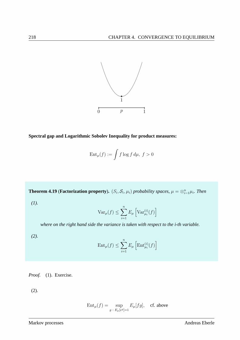
218 CHAPTER 4. CONVERGENCE TO EQUILIBRIUM
| |
0 1p
b
1
Spectral gap and Logarithmic Sobolev Inequality for productmeasures:
Entµ(f) :=
ˆ
f log f dµ, f > 0
Theorem 4.19(Factorization property ). (Si,Si, µi) probability spaces,µ = ⊗ni=1µi. Then
(1).
Varµ(f) ≤n∑
i=1
Eµ
[Var(i)µi
(f)]
where on the right hand side the variance is taken with respect to the i-th variable.
(2).
Entµ(f) ≤n∑
i=1
Eµ
[Ent(i)µi
(f)]
Proof. (1). Exercise.
(2).
Entµ(f) = supg : Eµ[eg ]=1
Eµ[fg], cf. above
Markov processes Andreas Eberle
4.4. LOGARITHMIC SOBOLEV INEQUALITIES AND ENTROPY BOUDS 219
Fix g : Sn → R such thatEµ [eg] = 1. Decompose:
g(x1, . . . , xn) = log eg(x1,...,xn)
= logeg(x1,...,xn)
´
eg(y1,x2,...,xn) µ1(dy1)+ log
´
eg(y1,x2,...,xn) µ1(dy1)˜
eg(y1,y2,x3,...,xn) µ1(dy1)µ2(dy2)+ · · ·
=:n∑
i=1
gi(x1, . . . , xn)
and hence
Eiµi[egi ] = 1 ∀, 1 ≤ i ≤ n
⇒ Eµ[fg] =n∑
i=1
Eµ [fgi] =n∑
i=1
Eµ
[E(i)
µi[fgi]
]≤ Ent(i)µi
(f)
⇒ Entµ[f ] = supEµ[eg ]=1
Eµ[fg] ≤n∑
i=1
Eµ
[Ent(i)µi
(f)]
Corollary 4.20. (1). If the Poincaré inequalities
Varµi(f) ≤ 1
λiEi(f, f) ∀ f ∈ Ai
hold for eachµi then
Varµ(f) ≤1
λE(f, f) ∀ f ∈
n⊗
i=1
Ai
where
E(f, f) =n∑
i=1
Eµ
[E (i)i (f, f)
]
and
λ = min1≤i≤n
λi
(2). The corresponding assertion holds for Logarithmic Sobolev Inequalities withα = maxαi
Proof.
Varµ(f) ≤n∑
i=1
Eµ
[Var(i)µi
(f)]≤ 1
minλiE(f, f)
since
Var(i)µi(f) ≤ 1
λiEi(f, f)
University of Bonn Winter term 2014/2015
220 CHAPTER 4. CONVERGENCE TO EQUILIBRIUM
Example. S = 0, 1n, µn product ofBernoulli(p),
Entµn(f 2)
≤ 2α(p)·p·q ·n∑
i=1
ˆ
|f(x1, . . . , xi−1, 1, xi+1, . . . , xn)− f(x1, . . . , xi−1, 0, xi+1, . . . , xn)|2 µn(dx)
independent ofn.
Example. Standard normal distributionγ = N(0, 1),
ϕn : 0, 1n → R, ϕn(x) =
∑ni=1
(xi − 1
2
)√
n4
The Central Limit Theorem yields thatµ = Bernoulli(12) and hence
µn ϕ−1n
w→ γ
Hence for allf ∈ C∞0 (R),
Entγ(f2) = lim
n→∞Entµn(f 2 ϕn)
≤ lim inf1
2
n∑
i=1
ˆ
|∆if ϕn|2 dµn
≤ · · · ≤ 2 ·ˆ
|f ′|2 dγ
4.4.4 LSI for log-concave probability measures
Stochastic gradient flow inRn:
dXt = dBt − (∇H)(Xt) dt, H ∈ C2(Rn)
Generator:
L =1
2∆−∇H · ∇
µ(dx) = e−H(x) dx satisfiesL∗µ = 0
Assumption: There exists aκ > 0 such that
∂2H(x) ≥ κ · I ∀ x ∈ Rn
i.e. ∂2ξξH ≥ κ · |ξ|2 ∀ ξ ∈ Rn
Markov processes Andreas Eberle
4.4. LOGARITHMIC SOBOLEV INEQUALITIES AND ENTROPY BOUDS 221
Remark. The assumption implies the inequalities
x · ∇H(x) ≥ κ · |x|2 − c, (4.4.2)
H(x) ≥ κ
2|x|2 − c (4.4.3)
with constantsc, c ∈ R. By (4.4.2) and a Lyapunov argument it can be shown thatXt does not ex-
plode in finite time and thatpt(A0) ⊆ A whereA0 = span (C∞0 (Rn), 1), A = span (S(Rn), 1).
By (4.4.3), the measureµ is finite, hence by our results above, the normalized measureis a
stationary distribution forpt.
Lemma 4.21. If HessH ≥ κI then
|∇ptf | ≤ e−κtpt |∇f | f ∈ C1b (R
n)
Remark. (1). Actually, both statements are equivalent.
(2). If we replaceRn by an arbitrary Riemannian manifold the same assertion holdsunder the
assumption
Ric+HessH ≥ κ · I
(Bochner-Lichnerowicz-Weitzenböck).
Informal analytic proof:
∇Lf = ∇ (∆−∇H · ∇) f
=(∆−∇H · ∇ − ∂2H
)∇f
=:
L operator on one-forms (vector fields)
This yields the evolution equation for∇ptf :
∂
∂t∇ptf = ∇ ∂
∂tptf = ∇Lptf =
L ∇ptf
and hence
∂
∂t|∇ptf | =
∂
∂t(∇ptf · ∇ptf)
12 =
(∂∂t∇ptf
)· ∇ptf
|∇ptf |
=
(L ∇ptf
)· ∇ptf
|∇ptf |≤ L∇ptf · ∇ptf
|∇ptf |− κ · |∇ptf |
2
|∇ptf |≤ · · · ≤ L |∇ptf | − κ |∇ptf |
University of Bonn Winter term 2014/2015
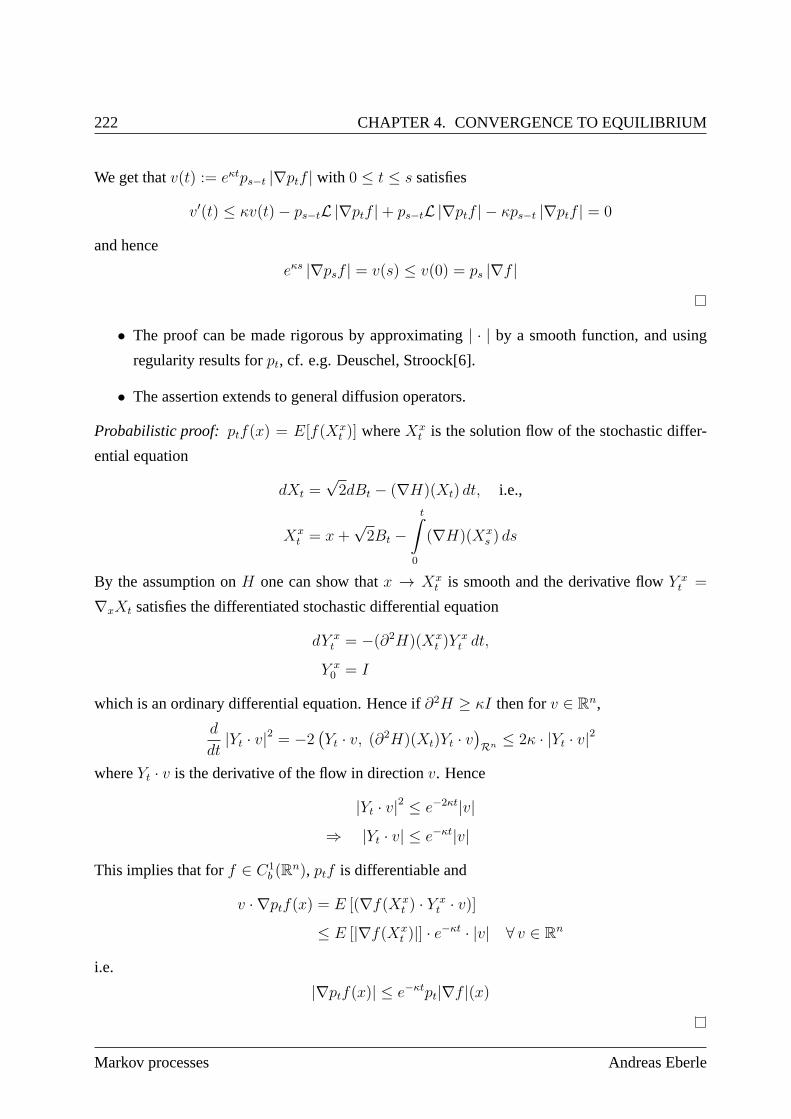
222 CHAPTER 4. CONVERGENCE TO EQUILIBRIUM
We get thatv(t) := eκtps−t |∇ptf | with 0 ≤ t ≤ s satisfies
v′(t) ≤ κv(t)− ps−tL |∇ptf |+ ps−tL |∇ptf | − κps−t |∇ptf | = 0
and hence
eκs |∇psf | = v(s) ≤ v(0) = ps |∇f |
• The proof can be made rigorous by approximating| · | by a smooth function, and using
regularity results forpt, cf. e.g. Deuschel, Stroock[6].
• The assertion extends to general diffusion operators.
Probabilistic proof: ptf(x) = E[f(Xxt )] whereXx
t is the solution flow of the stochastic differ-
ential equation
dXt =√2dBt − (∇H)(Xt) dt, i.e.,
Xxt = x+
√2Bt −
tˆ
0
(∇H)(Xxs ) ds
By the assumption onH one can show thatx → Xxt is smooth and the derivative flowY x
t =
∇xXt satisfies the differentiated stochastic differential equation
dY xt = −(∂2H)(Xx
t )Yxt dt,
Y x0 = I
which is an ordinary differential equation. Hence if∂2H ≥ κI then forv ∈ Rn,
d
dt|Yt · v|2 = −2
(Yt · v, (∂2H)(Xt)Yt · v
)Rn ≤ 2κ · |Yt · v|2
whereYt · v is the derivative of the flow in directionv. Hence
|Yt · v|2 ≤ e−2κt|v|⇒ |Yt · v| ≤ e−κt|v|
This implies that forf ∈ C1b (R
n), ptf is differentiable and
v · ∇ptf(x) = E [(∇f(Xxt ) · Y x
t · v)]≤ E [|∇f(Xx
t )|] · e−κt · |v| ∀ v ∈ Rn
i.e.
|∇ptf(x)| ≤ e−κtpt|∇f |(x)
Markov processes Andreas Eberle
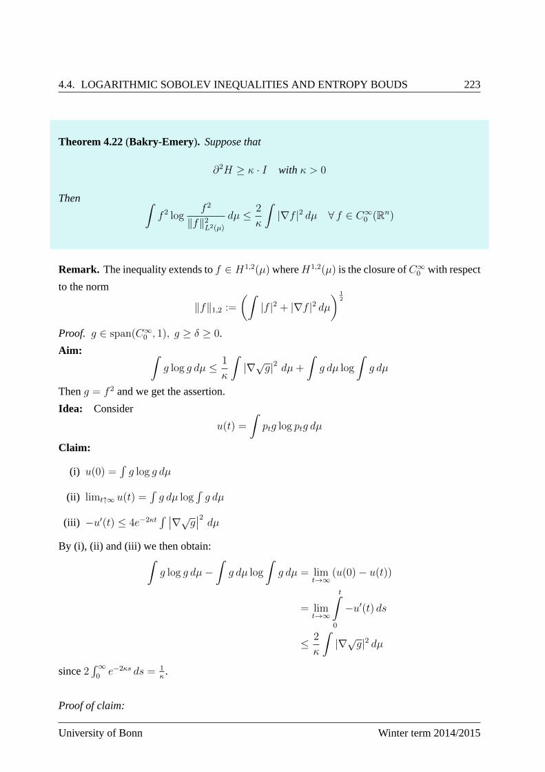
4.4. LOGARITHMIC SOBOLEV INEQUALITIES AND ENTROPY BOUDS 223
Theorem 4.22(Bakry-Emery ). Suppose that
∂2H ≥ κ · I with κ > 0
Thenˆ
f 2 logf 2
‖f‖2L2(µ)
dµ ≤ 2
κ
ˆ
|∇f |2 dµ ∀ f ∈ C∞0 (Rn)
Remark. The inequality extends tof ∈ H1,2(µ) whereH1,2(µ) is the closure ofC∞0 with respect
to the norm
‖f‖1,2 :=(ˆ
|f |2 + |∇f |2 dµ) 1
2
Proof. g ∈ span(C∞0 , 1), g ≥ δ ≥ 0.
Aim:ˆ
g log g dµ ≤ 1
κ
ˆ
|∇√g|2 dµ+
ˆ
g dµ log
ˆ
g dµ
Theng = f 2 and we get the assertion.
Idea: Consider
u(t) =
ˆ
ptg log ptg dµ
Claim:
(i) u(0) =´
g log g dµ
(ii) limt↑∞ u(t) =´
g dµ log´
g dµ
(iii) −u′(t) ≤ 4e−2κt´∣∣∇√
g∣∣2 dµ
By (i), (ii) and (iii) we then obtain:ˆ
g log g dµ−ˆ
g dµ log
ˆ
g dµ = limt→∞
(u(0)− u(t))
= limt→∞
tˆ
0
−u′(t) ds
≤ 2
κ
ˆ
|∇√g|2 dµ
since2´∞0e−2κs ds = 1
κ.
Proof of claim:
University of Bonn Winter term 2014/2015
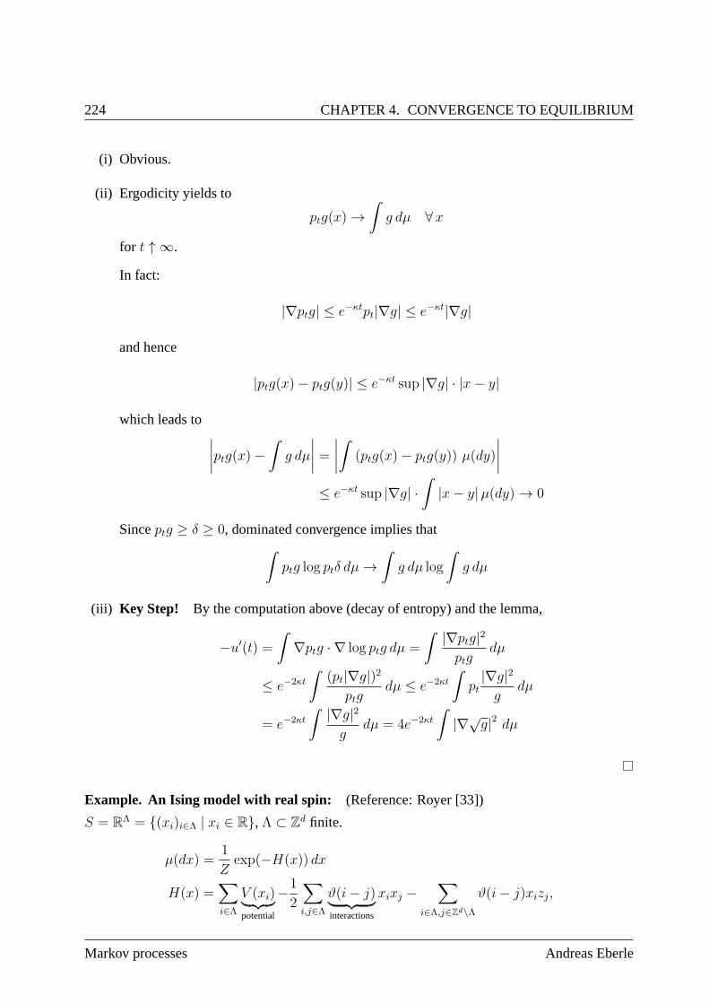
224 CHAPTER 4. CONVERGENCE TO EQUILIBRIUM
(i) Obvious.
(ii) Ergodicity yields to
ptg(x) →ˆ
g dµ ∀ x
for t ↑ ∞.
In fact:
|∇ptg| ≤ e−κtpt|∇g| ≤ e−κt|∇g|
and hence
|ptg(x)− ptg(y)| ≤ e−κt sup |∇g| · |x− y|
which leads to∣∣∣∣ptg(x)−
ˆ
g dµ
∣∣∣∣ =∣∣∣∣ˆ
(ptg(x)− ptg(y)) µ(dy)
∣∣∣∣
≤ e−κt sup |∇g| ·ˆ
|x− y|µ(dy) → 0
Sinceptg ≥ δ ≥ 0, dominated convergence implies thatˆ
ptg log ptδ dµ→ˆ
g dµ log
ˆ
g dµ
(iii) Key Step! By the computation above (decay of entropy) and the lemma,
−u′(t) =ˆ
∇ptg · ∇ log ptg dµ =
ˆ |∇ptg|2ptg
dµ
≤ e−2κt
ˆ
(pt|∇g|)2ptg
dµ ≤ e−2κt
ˆ
pt|∇g|2g
dµ
= e−2κt
ˆ |∇g|2g
dµ = 4e−2κt
ˆ
|∇√g|2 dµ
Example. An Ising model with real spin: (Reference: Royer [33])
S = RΛ = (xi)i∈Λ | xi ∈ R, Λ ⊂ Zd finite.
µ(dx) =1
Zexp(−H(x)) dx
H(x) =∑
i∈ΛV (xi)︸ ︷︷ ︸potential
−1
2
∑
i,j∈Λϑ(i− j)︸ ︷︷ ︸interactions
xixj −∑
i∈Λ,j∈Zd\Λ
ϑ(i− j)xizj,
Markov processes Andreas Eberle
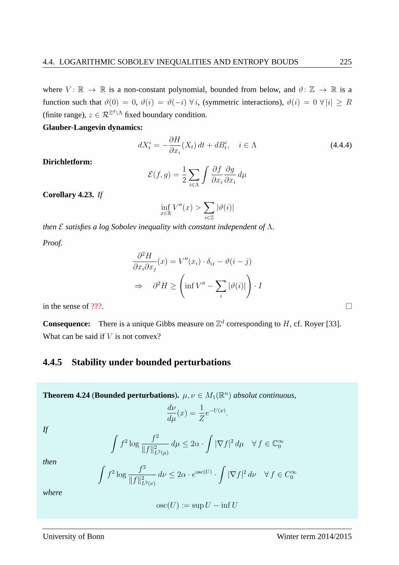
4.4. LOGARITHMIC SOBOLEV INEQUALITIES AND ENTROPY BOUDS 225
whereV : R → R is a non-constant polynomial, bounded from below, andϑ : Z → R is a
function such thatϑ(0) = 0, ϑ(i) = ϑ(−i) ∀ i, (symmetric interactions),ϑ(i) = 0 ∀ |i| ≥ R
(finite range),z ∈ RZd\Λ fixed boundary condition.
Glauber-Langevin dynamics:
dX it = −∂H
∂xi(Xt) dt+ dBi
t, i ∈ Λ (4.4.4)
Dirichletform:
E(f, g) = 1
2
∑
i∈Λ
ˆ
∂f
∂xi
∂g
∂xidµ
Corollary 4.23. If
infx∈R
V ′′(x) >∑
i∈Z|ϑ(i)|
thenE satisfies a log Sobolev inequality with constant independentof Λ.
Proof.
∂2H
∂xi∂xj(x) = V ′′(xi) · δij − ϑ(i− j)
⇒ ∂2H ≥(inf V ′′ −
∑
i
|ϑ(i)|)
· I
in the sense of???.
Consequence: There is a unique Gibbs measure onZd corresponding toH, cf. Royer [33].
What can be said ifV is not convex?
4.4.5 Stability under bounded perturbations
Theorem 4.24(Bounded perturbations). µ, ν ∈M1(Rn) absolut continuous,
dν
dµ(x) =
1
Ze−U(x).
Ifˆ
f 2 logf 2
‖f‖2L2(µ)
dµ ≤ 2α ·ˆ
|∇f |2 dµ ∀ f ∈ C∞0
thenˆ
f 2 logf 2
‖f‖2L2(ν)
dν ≤ 2α · eosc(U) ·ˆ
|∇f |2 dν ∀ f ∈ C∞0
where
osc(U) := supU − inf U
University of Bonn Winter term 2014/2015
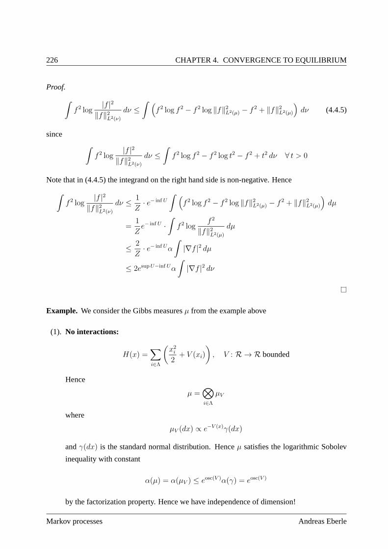
226 CHAPTER 4. CONVERGENCE TO EQUILIBRIUM
Proof.
ˆ
f 2 log|f |2
‖f‖2L2(ν)
dν ≤ˆ (
f 2 log f 2 − f 2 log ‖f‖2L2(µ) − f 2 + ‖f‖2L2(µ)
)dν (4.4.5)
sinceˆ
f 2 log|f |2
‖f‖2L2(ν)
dν ≤ˆ
f 2 log f 2 − f 2 log t2 − f 2 + t2 dν ∀ t > 0
Note that in (4.4.5) the integrand on the right hand side is non-negative. Hence
ˆ
f 2 log|f |2
‖f‖2L2(ν)
dν ≤ 1
Z· e− inf U
ˆ (f 2 log f 2 − f 2 log ‖f‖2L2(µ) − f 2 + ‖f‖2L2(µ)
)dµ
=1
Ze− inf U ·
ˆ
f 2 logf 2
‖f‖2L2(µ)
dµ
≤ 2
Z· e− inf Uα
ˆ
|∇f |2 dµ
≤ 2esupU−inf Uα
ˆ
|∇f |2 dν
Example. We consider the Gibbs measuresµ from the example above
(1). No interactions:
H(x) =∑
i∈Λ
(x2i2
+ V (xi)
), V : R → R bounded
Hence
µ =⊗
i∈ΛµV
where
µV (dx) ∝ e−V (x)γ(dx)
andγ(dx) is the standard normal distribution. Henceµ satisfies the logarithmic Sobolev
inequality with constant
α(µ) = α(µV ) ≤ eosc(V )α(γ) = eosc(V )
by the factorization property. Hence we have independence of dimension!
Markov processes Andreas Eberle
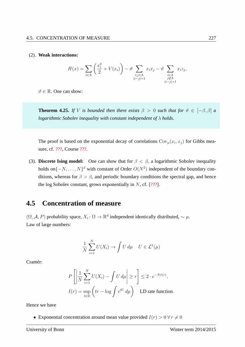
4.5. CONCENTRATION OF MEASURE 227
(2). Weak interactions:
H(x) =∑
i∈Λ
(x2i2
+ V (xi)
)− ϑ
∑
i,j∈Λ|i−j|=1
xixj − ϑ∑
i∈Λj /∈Λ
|i−j|=1
xizj,
ϑ ∈ R. One can show:
Theorem 4.25. If V is bounded then there existsβ > 0 such that forϑ ∈ [−β, β] a
logarithmic Sobolev inequality with constant independent of λ holds.
The proof is based on the exponential decay of correlationsCovµ(xi, xj) for Gibbs mea-
sure, cf.???, Course???.
(3). Discrete Ising model: One can show that forβ < βc a logarithmic Sobolev inequality
holds on−N, . . . , Nd with constant of OrderO(N2) independent of the boundary con-
ditions, whereas forβ > βc and periodic boundary conditions the spectral gap, and hence
the log Sobolev constant, grows exponentially inN , cf. [???].
4.5 Concentration of measure
(Ω,A, P ) probability space,Xi : Ω → Rd independent identically distributed,∼ µ.
Law of large numbers:
1
N
N∑
i=1
U(Xi) →ˆ
U dµ U ∈ L1(µ)
Cramér:
P
[∣∣∣∣∣1
N
N∑
i=1
U(Xi)−ˆ
U dµ
∣∣∣∣∣ ≥ r
]≤ 2 · e−NI(r),
I(r) = supt∈R
(tr − log
ˆ
etU dµ
)LD rate function.
Hence we have
• Exponential concentration around mean value providedI(r) > 0 ∀ r 6= 0
University of Bonn Winter term 2014/2015
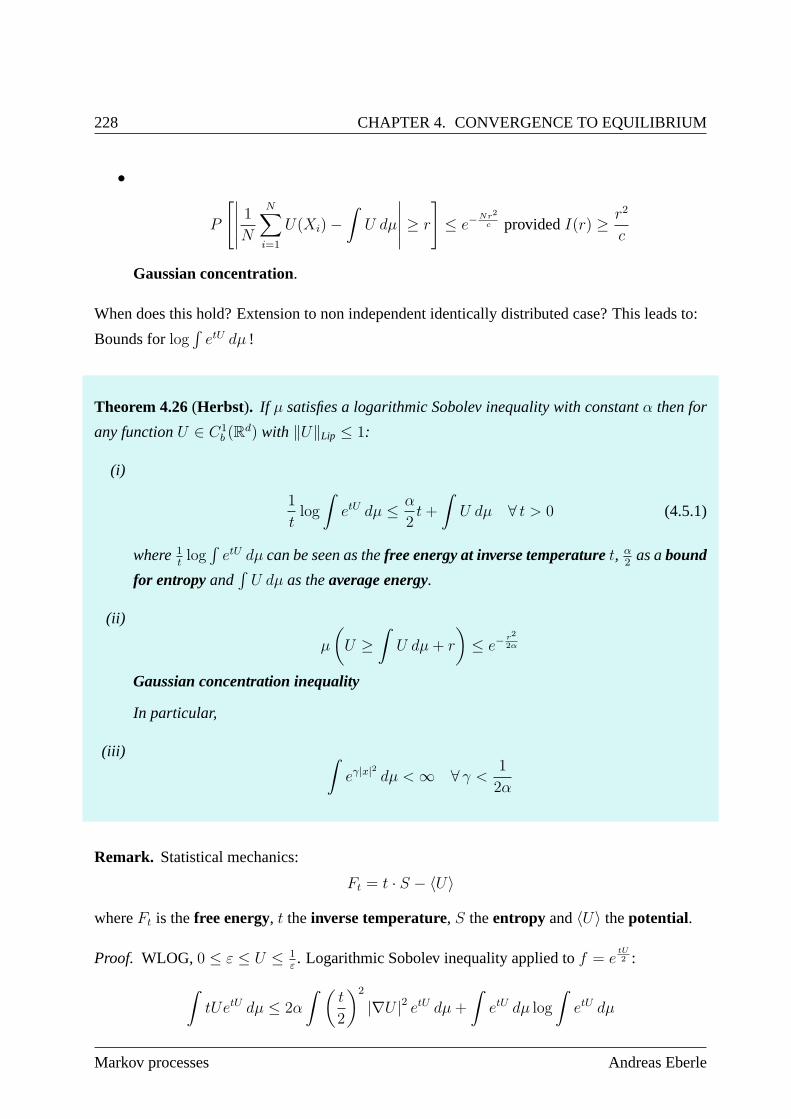
228 CHAPTER 4. CONVERGENCE TO EQUILIBRIUM
•
P
[∣∣∣∣∣1
N
N∑
i=1
U(Xi)−ˆ
U dµ
∣∣∣∣∣ ≥ r
]≤ e−
Nr2
c providedI(r) ≥ r2
c
Gaussian concentration.
When does this hold? Extension to non independent identically distributed case? This leads to:
Bounds forlog´
etU dµ !
Theorem 4.26(Herbst). If µ satisfies a logarithmic Sobolev inequality with constantα then for
any functionU ∈ C1b (R
d) with ‖U‖Lip ≤ 1:
(i)
1
tlog
ˆ
etU dµ ≤ α
2t+
ˆ
U dµ ∀ t > 0 (4.5.1)
where1tlog´
etU dµ can be seen as thefree energy at inverse temperaturet, α2
as abound
for entropyand´
U dµ as theaverage energy.
(ii)
µ
(U ≥
ˆ
U dµ+ r
)≤ e−
r2
2α
Gaussian concentration inequality
In particular,
(iii)ˆ
eγ|x|2
dµ <∞ ∀ γ < 1
2α
Remark. Statistical mechanics:
Ft = t · S − 〈U〉
whereFt is thefree energy, t the inverse temperature, S theentropy and〈U〉 thepotential.
Proof. WLOG, 0 ≤ ε ≤ U ≤ 1ε. Logarithmic Sobolev inequality applied tof = e
tU2 :
ˆ
tUetU dµ ≤ 2α
ˆ(t
2
)2
|∇U |2 etU dµ+
ˆ
etU dµ log
ˆ
etU dµ
Markov processes Andreas Eberle
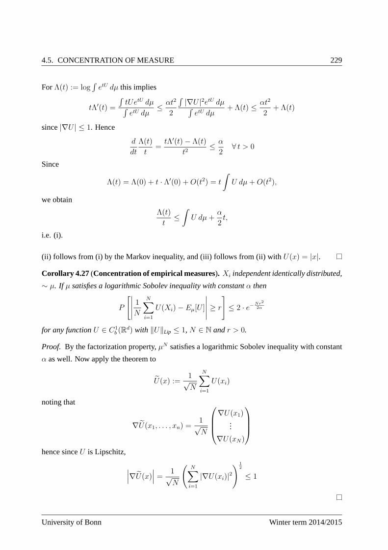
4.5. CONCENTRATION OF MEASURE 229
ForΛ(t) := log´
etU dµ this implies
tΛ′(t) =
´
tUetU dµ´
etU dµ≤ αt2
2
´
|∇U |2etU dµ´
etU dµ+ Λ(t) ≤ αt2
2+ Λ(t)
since|∇U | ≤ 1. Hence
d
dt
Λ(t)
t=tΛ′(t)− Λ(t)
t2≤ α
2∀ t > 0
Since
Λ(t) = Λ(0) + t · Λ′(0) +O(t2) = t
ˆ
U dµ+O(t2),
we obtain
Λ(t)
t≤ˆ
U dµ+α
2t,
i.e. (i).
(ii) follows from (i) by the Markov inequality, and (iii) follows from (ii) withU(x) = |x|.
Corollary 4.27 (Concentration of empirical measures). Xi independent identically distributed,
∼ µ. If µ satisfies a logarithmic Sobolev inequality with constantα then
P
[∣∣∣∣∣1
N
N∑
i=1
U(Xi)− Eµ[U ]
∣∣∣∣∣ ≥ r
]≤ 2 · e−Nr2
2α
for any functionU ∈ C1b (R
d) with ‖U‖Lip ≤ 1,N ∈ N andr > 0.
Proof. By the factorization property,µN satisfies a logarithmic Sobolev inequality with constant
α as well. Now apply the theorem to
U(x) :=1√N
N∑
i=1
U(xi)
noting that
∇U(x1, . . . , xn) =1√N
∇U(x1)...
∇U(xN)
hence sinceU is Lipschitz,
∣∣∣∇U(x)∣∣∣ = 1√
N
(N∑
i=1
|∇U(xi)|2) 1
2
≤ 1
University of Bonn Winter term 2014/2015
Appendix
Let (Ω,A, P ) be a probability space, we denote byL1(Ω,A, P ) (L1(P )) the space of measurable
random variablesX : Ω → R with E[X−] < ∞ andL1(P ) := L1(P )/ ∼ where two random
variables a in relation to each other, if they are equal almost everywhere.
A.1 Conditional expectation
For more details and proofs of the following statements see [Eberle:Stochastic processes] [10].
Definition (Conditional expectations). LetX ∈ L1(Ω,A, P ) (or non-negative) andF ⊂ A a
σ-algebra. A random variableZ ∈ L1(Ω,F , P ) is calledconditional expectationofX givenF(writtenZ = E[X|F ]), if
• Z is F-measurable, and
• for all B ∈ F ,ˆ
B
ZdP =
ˆ
B
XdP.
The random variableE[X|F ] is P -a.s. unique. For a measurable Space(S,S) and an abritatry
random variableY : Ω → S we defineE[X|Y ] := E[X|σ(Y )] and there exists aP -a.s. unique
measurable functiong : S → R such thatE[X|σ(Y )] = g(Y ). One also sometimes defines
E[X|Y = y] := g(y) µY -a.e. (µY law ofY ).
Theorem A.1. Let X, Y andXn(n ∈ N) be non-negative or integrable random variables on
(Ω,A, P ) andF ,G ⊂ A twoσ-algebras. The following statements hold:
230
A.2. MARTINGALES 231
(1). Linearity:E[λX + µY |F ] = λE[X|F ] + µE[Y |F ] P -almost surely for allλ, µ ∈ R.
(2). Monotonicity:X ≥ 0 P -almost surely implies thatE[X|F ] ≥ 0 P -almost surely.
(3). X = Y P -almost surely implies thatE[X|F ] = E[Y |F ] P -almost surely.
(4). Monotone convergence: If(Xn) is growing monotone withX1 ≥ 0, then
E[supXn|F ] = supE[Xn|F ] P -almost surely.
(5). Projectivity / Tower property: IfG ⊂ F , then
E[E[X|F ]|G] = E[X|G] P -almost surely.
In particular:
E[E[X|Y, Z]|Y ] = E[X|Y ] P -almost surely.
(6). LetY beF-measurable withY ·X ∈ L1 or ≥ 0. This implies that
E[Y ·X|F ] = Y · E[X|F ] P -almost surely.
(7). Independence: IfX is independent ofF , thenE[X|F ] = E[X] P -almost surely.
(8). Let(S,S) and(T, T ) be two measurable spaces. IfY : Ω → S is F-measurable,
X : Ω → T independent ofF andf : S × T → [0,∞) a product measurable map, then it
holds that
E[f(X, Y )|F ](ω) = E[f(X, Y (ω))] for P -almost allω
Definition (Conditional probability ). Let(Ω,A, P ) be a probability space,F a σ-algebra. The
conditional probabilityis defined as
P [A|F ](ω) := E[1A|F ](ω) ∀A ∈ F , ω ∈ Ω.
A.2 Martingales
Classical analysis starts with studying convergence of sequences of real numbers. Similarly,
stochastic analysis relies on basic statements about sequences of real-valued random variables.
Any such sequence can be decomposed uniquely into a martingale, i.e., a real.valued stochastic
University of Bonn Winter term 2014/2015
232 CHAPTER A. APPENDIX
process that is “constant on average”, and a predictable part. Therefore, estimates and conver-
gence theorems for martingales are crucial in stochastic analysis.
A.2.1 Filtrations
We fix a probability space(Ω,A, P ). Moreover, we assume that we are given an increasing
sequenceFn (n = 0, 1, 2, . . .) of sub-σ-algebras ofA. Intuitively, we often think ofFn as
describing the information available to us at timen. Formally, we define:
Definition (Filtration, adapted process). (1). A filtration on(Ω,A) is an increasing sequence
F0 ⊆ F1 ⊆ F2 ⊆ . . .
of σ-algebrasFn ⊆ A.
(2). A stochastic process(Xn)n≥0 is adapted to a filtration(Fn)n≥0 iff eachXn isFn-measurable.
Example. (1). Thecanonical filtration(FXn ) generated by a stochastic process(Xn) is given
by
FXn = σ(X0, X1, . . . , Xn).
If the filtration is not specified explicitly, we will usuallyconsider the canonical filtration.
(2). Alternatively, filtrations containing additional information are of interest, for example the
filtration
Fn = σ(Z,X0, X1, . . . , Xn)
generated by the process(Xn) and an additional random variableZ, or the filtration
Fn = σ(X0, Y0, X1, Y1, . . . , Xn, Yn)
generated by the process(Xn) and a further process(Yn). Clearly, the process(Xn) is
adapted to any of these filtrations. In general,(Xn) is adapted to a filtration(Fn) if and
only if FXn ⊆ Fn for anyn ≥ 0.
A.2.2 Martingales and supermartingales
We can now formalize the notion of a real-valued stochastic process that is constant (respectively
decreasing or increasing) on average:
Definition (Martingale, supermartingale, submartingale).
Markov processes Andreas Eberle
A.2. MARTINGALES 233
(1). A sequence of real-valued random variablesMn : Ω → R (n = 0, 1, . . .) on the proba-
bility space(Ω,A, P ) is called a martingale w.r.t. the filtration(Fn) if and only if
(a) (Mn) is adapted w.r.t.(Fn),
(b) Mn is integrable for anyn ≥ 0, and
(c) E[Mn | Fn−1] = Mn−1 for anyn ∈ N.
(2). Similarly,(Mn) is called a supermartingale (resp. a submartingale) w.r.t.(Fn), if and only
if (a) holds, the positive partM+n (resp. the negative partM−
n ) is integrable for anyn ≥ 0,
and (c) holds with “=” replaced by “≤”, “ ≥” respectively.
Condition (c) in the martingale definition can equivalently be written as
(c’) E[Mn+1 −Mn | Fn] = 0 for anyn ∈ Z+,
and correspondingly with “=” replaced by “≤” or “≥” for super- or submartingales.
Intuitively, a martingale is a ”fair gameÅ12Å 1
2, i.e.,Mn−1 is the best prediction (w.r.t. the mean
square error) for the next valueMn given the information up to timen − 1. A supermartingale
is “decreasingon average”, a submartingale is“increasingon average”, and a martingale is both
“decreasing” and “increasing”, i.e.,“constanton average”. In particular, by induction onn, a
martingale satisfies
E[Mn] = E[M0] for anyn ≥ 0.
Similarly, for a supermartingale, the expectation valuesE[Mn] are decreasing. More generally,
we have:
Lemma A.2. If (Mn) is a martingale (respectively a supermartingale) w.r.t. a filtration (Fn)
then
E[Mn+k | Fn](≤)= Mn P -almost surely for anyn, k ≥ 0.
A.2.3 Doob Decomposition
We will show now that any adapted sequence of real-valued random variables can be decomposed
into a martingale and a predictable process. In particular,the variance process of a martingale
(Mn) is the predictable part in the corresponding Doob decomposition of the process(M2n). The
Doob decomposition for functions of Markov chains implies the Martingale Problem characteri-
zation of Markov chains.
Let (Ω,A, P ) be a probability space and(Fn)n≥0 a filtration on(Ω,A).
University of Bonn Winter term 2014/2015
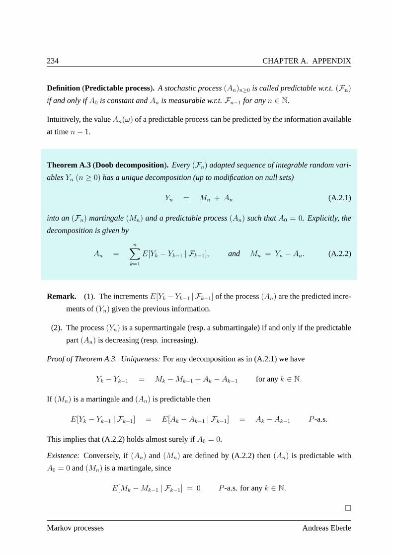
234 CHAPTER A. APPENDIX
Definition (Predictable process). A stochastic process(An)n≥0 is called predictable w.r.t.(Fn)
if and only ifA0 is constant andAn is measurable w.r.t.Fn−1 for anyn ∈ N.
Intuitively, the valueAn(ω) of a predictable process can be predicted by the informationavailable
at timen− 1.
Theorem A.3(Doob decomposition). Every(Fn) adapted sequence of integrable random vari-
ablesYn (n ≥ 0) has a unique decomposition (up to modification on null sets)
Yn = Mn + An (A.2.1)
into an(Fn) martingale(Mn) and a predictable process(An) such thatA0 = 0. Explicitly, the
decomposition is given by
An =n∑
k=1
E[Yk − Yk−1 | Fk−1], and Mn = Yn − An. (A.2.2)
Remark. (1). The incrementsE[Yk − Yk−1 | Fk−1] of the process(An) are the predicted incre-
ments of(Yn) given the previous information.
(2). The process(Yn) is a supermartingale (resp. a submartingale) if and only if the predictable
part(An) is decreasing (resp. increasing).
Proof of Theorem A.3. Uniqueness:For any decomposition as in (A.2.1) we have
Yk − Yk−1 = Mk −Mk−1 + Ak − Ak−1 for anyk ∈ N.
If (Mn) is a martingale and(An) is predictable then
E[Yk − Yk−1 | Fk−1] = E[Ak − Ak−1 | Fk−1] = Ak − Ak−1 P -a.s.
This implies that (A.2.2) holds almost surely ifA0 = 0.
Existence:Conversely, if(An) and(Mn) are defined by (A.2.2) then(An) is predictable with
A0 = 0 and(Mn) is a martingale, since
E[Mk −Mk−1 | Fk−1] = 0 P -a.s. for anyk ∈ N.
Markov processes Andreas Eberle
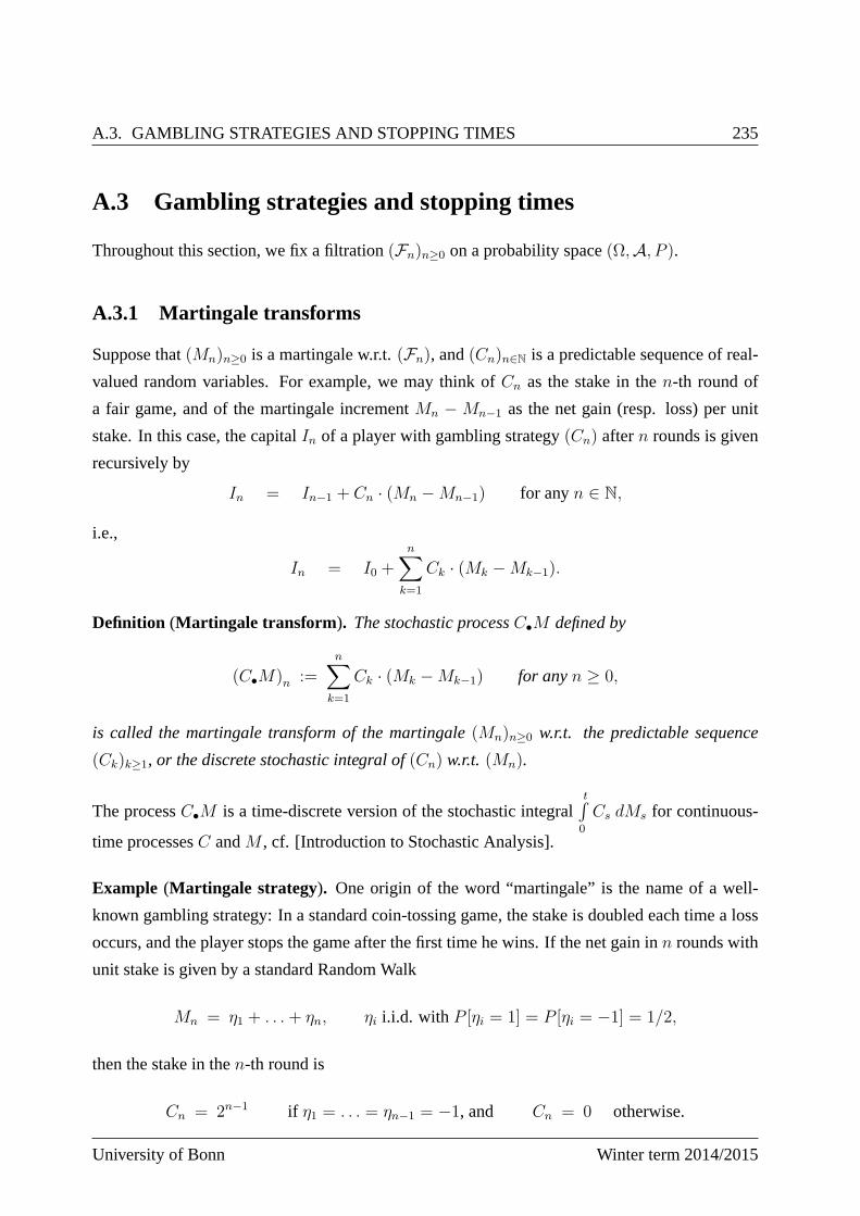
A.3. GAMBLING STRATEGIES AND STOPPING TIMES 235
A.3 Gambling strategies and stopping times
Throughout this section, we fix a filtration(Fn)n≥0 on a probability space(Ω,A, P ).
A.3.1 Martingale transforms
Suppose that(Mn)n≥0 is a martingale w.r.t.(Fn), and(Cn)n∈N is a predictable sequence of real-
valued random variables. For example, we may think ofCn as the stake in then-th round of
a fair game, and of the martingale incrementMn −Mn−1 as the net gain (resp. loss) per unit
stake. In this case, the capitalIn of a player with gambling strategy(Cn) aftern rounds is given
recursively by
In = In−1 + Cn · (Mn −Mn−1) for anyn ∈ N,
i.e.,
In = I0 +n∑
k=1
Ck · (Mk −Mk−1).
Definition (Martingale transform ). The stochastic processC•M defined by
(C•M)n :=n∑
k=1
Ck · (Mk −Mk−1) for anyn ≥ 0,
is called the martingale transform of the martingale(Mn)n≥0 w.r.t. the predictable sequence
(Ck)k≥1, or the discrete stochastic integral of(Cn) w.r.t. (Mn).
The processC•M is a time-discrete version of the stochastic integralt
0
Cs dMs for continuous-
time processesC andM , cf. [Introduction to Stochastic Analysis].
Example (Martingale strategy). One origin of the word “martingale” is the name of a well-
known gambling strategy: In a standard coin-tossing game, the stake is doubled each time a loss
occurs, and the player stops the game after the first time he wins. If the net gain inn rounds with
unit stake is given by a standard Random Walk
Mn = η1 + . . .+ ηn, ηi i.i.d. with P [ηi = 1] = P [ηi = −1] = 1/2,
then the stake in then-th round is
Cn = 2n−1 if η1 = . . . = ηn−1 = −1, and Cn = 0 otherwise.
University of Bonn Winter term 2014/2015

236 CHAPTER A. APPENDIX
Clearly, with probability one, the game terminates in finite time, and at that time the player has
always won one unit, i.e.,
P [(C•M)n = 1 eventually] = 1.
1
2
−1
−2
−3
−4
−5
−6
−7
n
(C•M)n
At first glance this looks like a safe winning strategy, but ofcourse this would only be the case,
if the player had unlimited capital and time available.
Theorem A.4 (You can’t beat the system!). (1). If (Mn)n≥0 is an (Fn) martingale, and
(Cn)n≥1 is predictable withCn · (Mn −Mn−1) ∈ L1(Ω,A, P ) for anyn ≥ 1, thenC•M is
again an(Fn) martingale.
(2). If (Mn) is an (Fn) supermartingale and(Cn)n≥1 is non-negative and predictable with
Cn · (Mn −Mn−1) ∈ L1 for anyn, thenC•M is again a supermartingale.
Markov processes Andreas Eberle
A.3. GAMBLING STRATEGIES AND STOPPING TIMES 237
Proof. Forn ≥ 1 we have
E[(C•M)n − (C•M)n−1 | Fn−1] = E[Cn · (Mn −Mn−1) | Fn−1]
= Cn · E[Mn −Mn−1 | Fn−1] = 0 P -a.s.
This proves the first part of the claim. The proof of the secondpart is similar.
The theorem shows that a fair game (a martingale) can not be transformed by choice of a clever
gambling strategy into an unfair (or “superfair”) game. In models of financial markets this fact is
crucial to exclude the existence of arbitrage possibilities (riskless profit).
Example (Martingale strategy, cont.). For the classical martingale strategy, we obtain
E[(C•M)n] = E[(C•M)0] = 0 for anyn ≥ 0
by the martingale property, although
limn→∞
(C•M)n = 1 P -a.s.
This is a classical example showing that the assertion of thedominated convergence theorem may
not hold if the assumptions are violated.
Remark. The integrability assumption in Theorem A.4 is always satisfied if the random variables
Cn are bounded, or if bothCn andMn are square-integrable for anyn.
A.3.2 Stopped Martingales
One possible strategy for controlling a fair game is to terminate the game at a time depending on
the previous development. Recall that a random variableT : Ω → 0, 1, 2, . . . ∪ ∞ is called
a stopping timew.r.t. the filtration(Fn) if and only if the eventT = n is contained inFn for
anyn ≥ 0, or equivalently, iffT ≤ n ∈ Fn for anyn ≥ 0.
We consider an(Fn)-adapted stochastic process(Mn)n≥0, and an(Fn)-stopping timeT on the
probability space(Ω,A, P ). The process stopped at timeT is defined as(MT∧n)n≥0 where
MT∧n(ω) = MT (ω)∧n(ω) =
Mn(ω) for n ≤ T (ω),
MT (ω)(ω) for n ≥ T (ω).
For example, the process stopped at a hitting timeTA gets stuck at the first time it enters the set
A.
University of Bonn Winter term 2014/2015
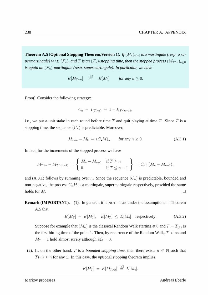
238 CHAPTER A. APPENDIX
Theorem A.5(Optional Stopping Theorem,Version 1). If (Mn)n≥0 is a martingale (resp. a su-
permartingale) w.r.t.(Fn), andT is an(Fn)-stopping time, then the stopped process(MT∧n)n≥0
is again an(Fn)-martingale (resp. supermartingale). In particular, we have
E[MT∧n](≤)= E[M0] for anyn ≥ 0.
Proof. Consider the following strategy:
Cn = IT≥n = 1− IT≤n−1,
i.e., we put a unit stake in each round before timeT and quit playing at timeT . SinceT is a
stopping time, the sequence(Cn) is predictable. Moreover,
MT∧n −M0 = (C•M)n for anyn ≥ 0. (A.3.1)
In fact, for the increments of the stopped process we have
MT∧n −MT∧(n−1) =
Mn −Mn−1 if T ≥ n
0 if T ≤ n− 1
= Cn · (Mn −Mn−1),
and (A.3.1) follows by summing overn. Since the sequence(Cn) is predictable, bounded and
non-negative, the processC•M is a martingale, supermartingale respectively, provided the same
holds forM .
Remark (IMPORTANT ). (1). In general, it isNOT TRUE under the assumptions in Theorem
A.5 that
E[MT ] = E[M0], E[MT ] ≤ E[M0] respectively. (A.3.2)
Suppose for example that(Mn) is the classical Random Walk starting at0 andT = T1 is
the first hitting time of the point1. Then, by recurrence of the Random Walk,T < ∞ and
MT = 1 hold almost surely althoughM0 = 0.
(2). If, on the other hand,T is a bounded stopping time, then there existsn ∈ N such that
T (ω) ≤ n for anyω. In this case, the optional stopping theorem implies
E[MT ] = E[MT∧n](≤)= E[M0].
Markov processes Andreas Eberle
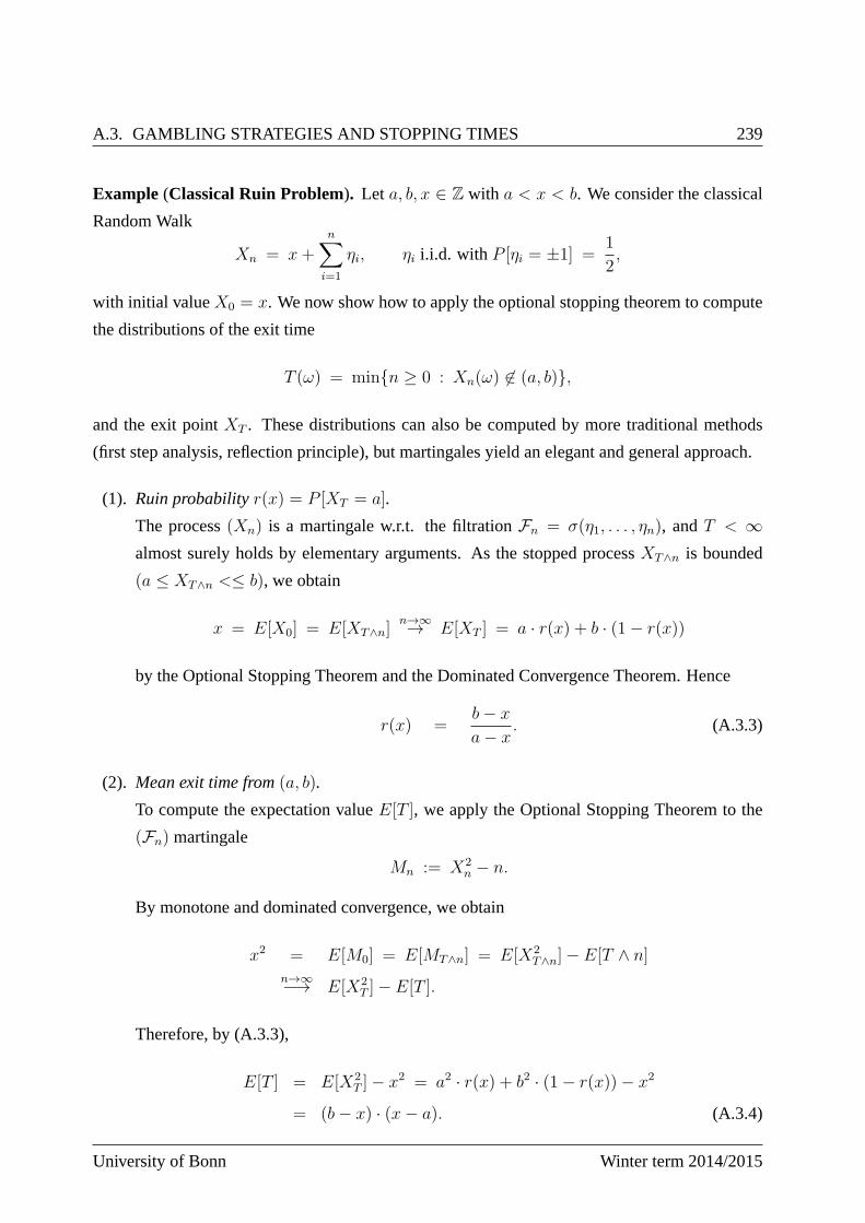
A.3. GAMBLING STRATEGIES AND STOPPING TIMES 239
Example (Classical Ruin Problem). Let a, b, x ∈ Z with a < x < b. We consider the classical
Random Walk
Xn = x+n∑
i=1
ηi, ηi i.i.d. with P [ηi = ±1] =1
2,
with initial valueX0 = x. We now show how to apply the optional stopping theorem to compute
the distributions of the exit time
T (ω) = minn ≥ 0 : Xn(ω) 6∈ (a, b),
and the exit pointXT . These distributions can also be computed by more traditional methods
(first step analysis, reflection principle), but martingales yield an elegant and general approach.
(1). Ruin probabilityr(x) = P [XT = a].
The process(Xn) is a martingale w.r.t. the filtrationFn = σ(η1, . . . , ηn), andT < ∞almost surely holds by elementary arguments. As the stoppedprocessXT∧n is bounded
(a ≤ XT∧n <≤ b), we obtain
x = E[X0] = E[XT∧n]n→∞→ E[XT ] = a · r(x) + b · (1− r(x))
by the Optional Stopping Theorem and the Dominated Convergence Theorem. Hence
r(x) =b− x
a− x. (A.3.3)
(2). Mean exit time from(a, b).
To compute the expectation valueE[T ], we apply the Optional Stopping Theorem to the
(Fn) martingale
Mn := X2n − n.
By monotone and dominated convergence, we obtain
x2 = E[M0] = E[MT∧n] = E[X2T∧n]− E[T ∧ n]
n→∞−→ E[X2T ]− E[T ].
Therefore, by (A.3.3),
E[T ] = E[X2T ]− x2 = a2 · r(x) + b2 · (1− r(x))− x2
= (b− x) · (x− a). (A.3.4)
University of Bonn Winter term 2014/2015
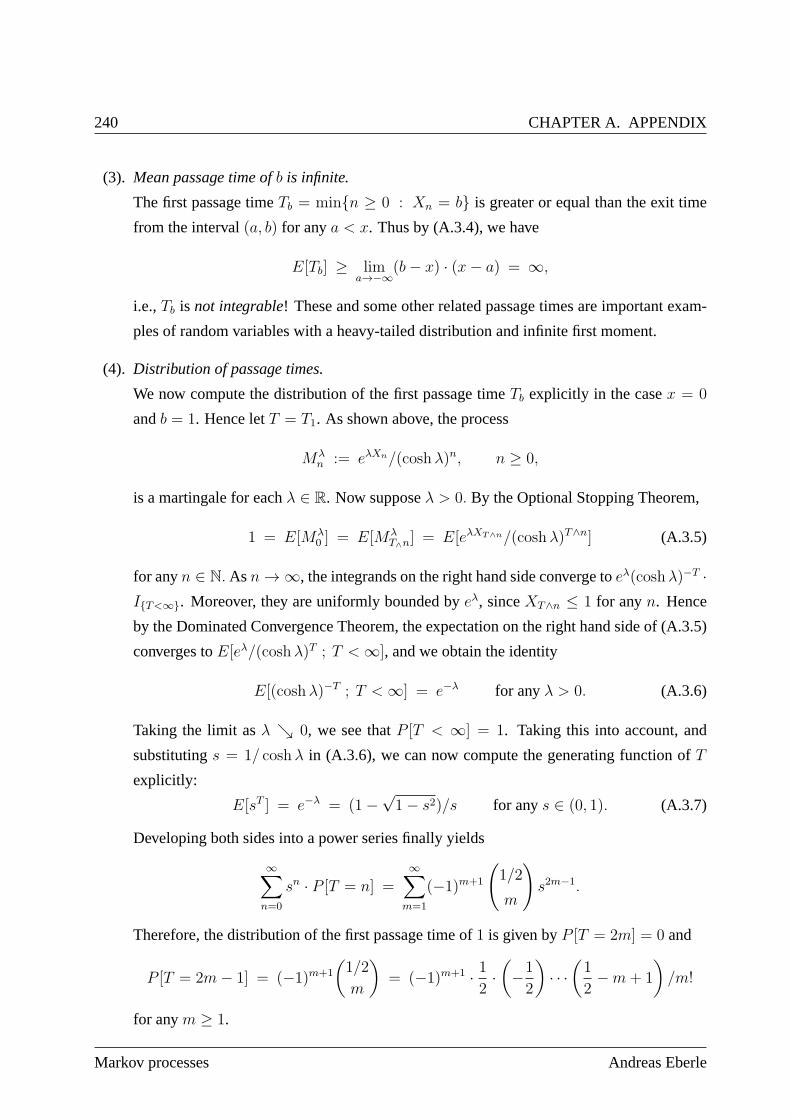
240 CHAPTER A. APPENDIX
(3). Mean passage time ofb is infinite.
The first passage timeTb = minn ≥ 0 : Xn = b is greater or equal than the exit time
from the interval(a, b) for anya < x. Thus by (A.3.4), we have
E[Tb] ≥ lima→−∞
(b− x) · (x− a) = ∞,
i.e.,Tb is not integrable! These and some other related passage times are important exam-
ples of random variables with a heavy-tailed distribution and infinite first moment.
(4). Distribution of passage times.
We now compute the distribution of the first passage timeTb explicitly in the casex = 0
andb = 1. Hence letT = T1. As shown above, the process
Mλn := eλXn/(coshλ)n, n ≥ 0,
is a martingale for eachλ ∈ R. Now supposeλ > 0. By the Optional Stopping Theorem,
1 = E[Mλ0 ] = E[Mλ
T∧n] = E[eλXT∧n/(coshλ)T∧n] (A.3.5)
for anyn ∈ N. Asn→ ∞, the integrands on the right hand side converge toeλ(coshλ)−T ·IT<∞. Moreover, they are uniformly bounded byeλ, sinceXT∧n ≤ 1 for anyn. Hence
by the Dominated Convergence Theorem, the expectation on theright hand side of (A.3.5)
converges toE[eλ/(coshλ)T ; T <∞], and we obtain the identity
E[(coshλ)−T ; T <∞] = e−λ for anyλ > 0. (A.3.6)
Taking the limit asλ ց 0, we see thatP [T < ∞] = 1. Taking this into account, and
substitutings = 1/ coshλ in (A.3.6), we can now compute the generating function ofT
explicitly:
E[sT ] = e−λ = (1−√1− s2)/s for anys ∈ (0, 1). (A.3.7)
Developing both sides into a power series finally yields
∞∑
n=0
sn · P [T = n] =∞∑
m=1
(−1)m+1
(1/2
m
)s2m−1.
Therefore, the distribution of the first passage time of1 is given byP [T = 2m] = 0 and
P [T = 2m− 1] = (−1)m+1
(1/2
m
)= (−1)m+1 · 1
2·(−1
2
)· · ·(1
2−m+ 1
)/m!
for anym ≥ 1.
Markov processes Andreas Eberle
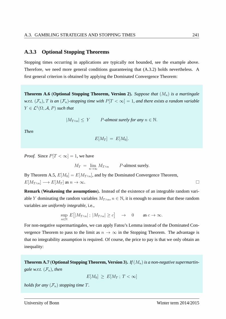
A.3. GAMBLING STRATEGIES AND STOPPING TIMES 241
A.3.3 Optional Stopping Theorems
Stopping times occurring in applications are typically notbounded, see the example above.
Therefore, we need more general conditions guaranteeing that (A.3.2) holds nevertheless. A
first general criterion is obtained by applying the Dominated Convergence Theorem:
Theorem A.6 (Optional Stopping Theorem, Version 2). Suppose that(Mn) is a martingale
w.r.t. (Fn), T is an(Fn)-stopping time withP [T < ∞] = 1, and there exists a random variable
Y ∈ L1(Ω,A, P ) such that
|MT∧n| ≤ Y P -almost surely for anyn ∈ N.
Then
E[MT ] = E[M0].
Proof. SinceP [T <∞] = 1, we have
MT = limn→∞
MT∧n P -almost surely.
By Theorem A.5,E[M0] = E[MT∧n], and by the Dominated Convergence Theorem,
E[MT∧n] −→ E[MT ] asn→ ∞.
Remark (Weakening the assumptions). Instead of the existence of an integrable random vari-
ableY dominating the random variablesMT∧n, n ∈ N, it is enough to assume that these random
variables areuniformly integrable, i.e.,
supn∈N
E[|MT∧n| ; |MT∧n| ≥ c
]→ 0 asc→ ∞.
For non-negative supermartingales, we can apply Fatou’s Lemma instead of the Dominated Con-
vergence Theorem to pass to the limit asn → ∞ in the Stopping Theorem. The advantage is
that no integrability assumption is required. Of course, the price to pay is that we only obtain an
inequality:
Theorem A.7(Optional Stopping Theorem, Version 3). If (Mn) is a non-negative supermartin-
gale w.r.t.(Fn), then
E[M0] ≥ E[MT ; T <∞]
holds for any(Fn) stopping timeT .
University of Bonn Winter term 2014/2015
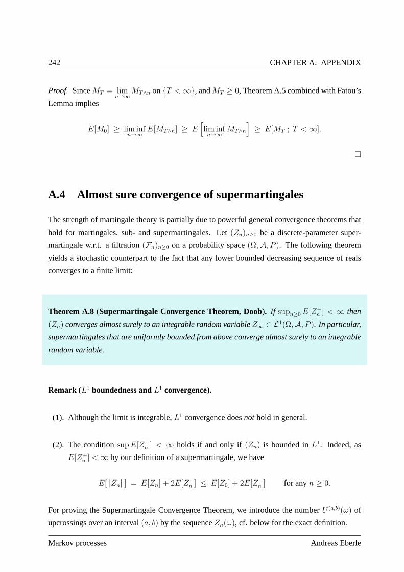
242 CHAPTER A. APPENDIX
Proof. SinceMT = limn→∞
MT∧n onT <∞, andMT ≥ 0, Theorem A.5 combined with Fatou’s
Lemma implies
E[M0] ≥ lim infn→∞
E[MT∧n] ≥ E[lim infn→∞
MT∧n
]≥ E[MT ; T <∞].
A.4 Almost sure convergence of supermartingales
The strength of martingale theory is partially due to powerful general convergence theorems that
hold for martingales, sub- and supermartingales. Let(Zn)n≥0 be a discrete-parameter super-
martingale w.r.t. a filtration(Fn)n≥0 on a probability space(Ω,A, P ). The following theorem
yields a stochastic counterpart to the fact that any lower bounded decreasing sequence of reals
converges to a finite limit:
Theorem A.8 (Supermartingale Convergence Theorem, Doob). If supn≥0E[Z−n ] < ∞ then
(Zn) converges almost surely to an integrable random variableZ∞ ∈ L1(Ω,A, P ). In particular,
supermartingales that are uniformly bounded from above converge almost surely to an integrable
random variable.
Remark (L1 boundedness andL1 convergence).
(1). Although the limit is integrable,L1 convergence doesnot hold in general.
(2). The conditionsupE[Z−n ] < ∞ holds if and only if(Zn) is bounded inL1. Indeed, as
E[Z+n ] <∞ by our definition of a supermartingale, we have
E[ |Zn| ] = E[Zn] + 2E[Z−n ] ≤ E[Z0] + 2E[Z−
n ] for anyn ≥ 0.
For proving the Supermartingale Convergence Theorem, we introduce the numberU (a,b)(ω) of
upcrossings over an interval(a, b) by the sequenceZn(ω), cf. below for the exact definition.
Markov processes Andreas Eberle
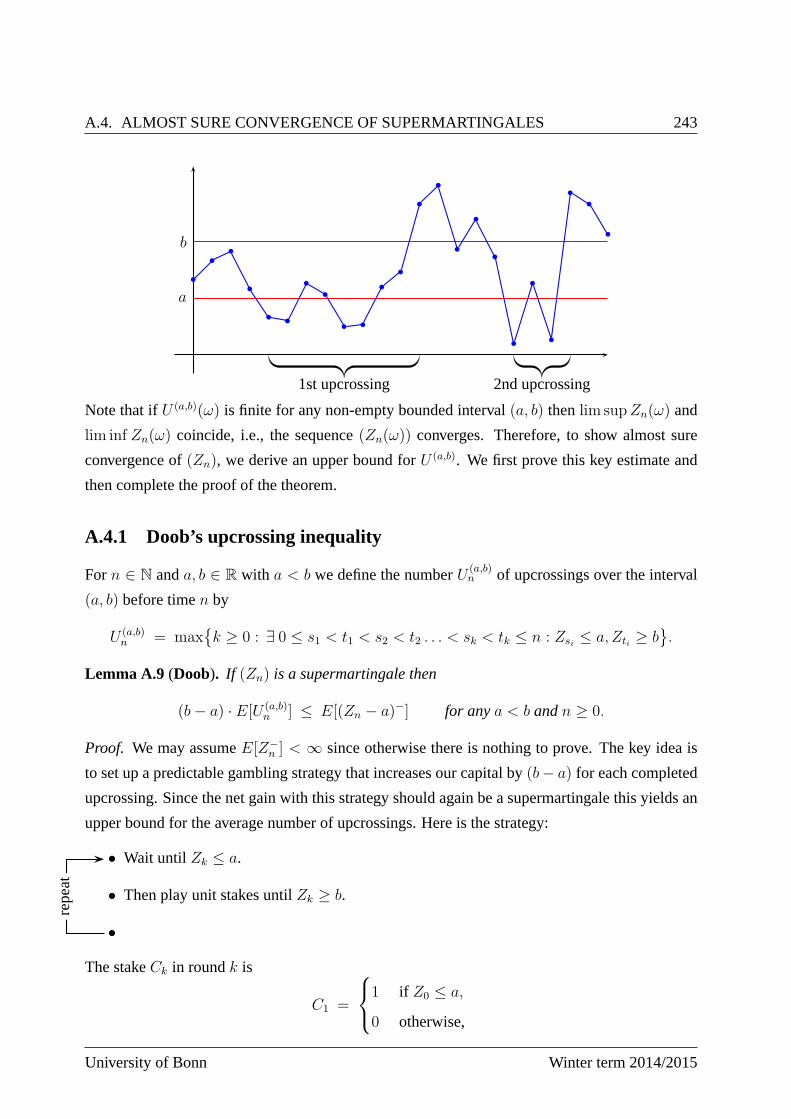
A.4. ALMOST SURE CONVERGENCE OF SUPERMARTINGALES 243
b
a
1st upcrossing 2nd upcrossing
Note that ifU (a,b)(ω) is finite for any non-empty bounded interval(a, b) thenlim supZn(ω) and
lim inf Zn(ω) coincide, i.e., the sequence(Zn(ω)) converges. Therefore, to show almost sure
convergence of(Zn), we derive an upper bound forU (a,b). We first prove this key estimate and
then complete the proof of the theorem.
A.4.1 Doob’s upcrossing inequality
Forn ∈ N anda, b ∈ R with a < b we define the numberU (a,b)n of upcrossings over the interval
(a, b) before timen by
U (a,b)n = max
k ≥ 0 : ∃ 0 ≤ s1 < t1 < s2 < t2 . . . < sk < tk ≤ n : Zsi ≤ a, Zti ≥ b
.
Lemma A.9 (Doob). If (Zn) is a supermartingale then
(b− a) · E[U (a,b)n ] ≤ E[(Zn − a)−] for anya < b andn ≥ 0.
Proof. We may assumeE[Z−n ] < ∞ since otherwise there is nothing to prove. The key idea is
to set up a predictable gambling strategy that increases ourcapital by(b− a) for each completed
upcrossing. Since the net gain with this strategy should again be a supermartingale this yields an
upper bound for the average number of upcrossings. Here is the strategy:
• Wait untilZk ≤ a.
• Then play unit stakes untilZk ≥ b.
•
repe
at
The stakeCk in roundk is
C1 =
1 if Z0 ≤ a,
0 otherwise,
University of Bonn Winter term 2014/2015
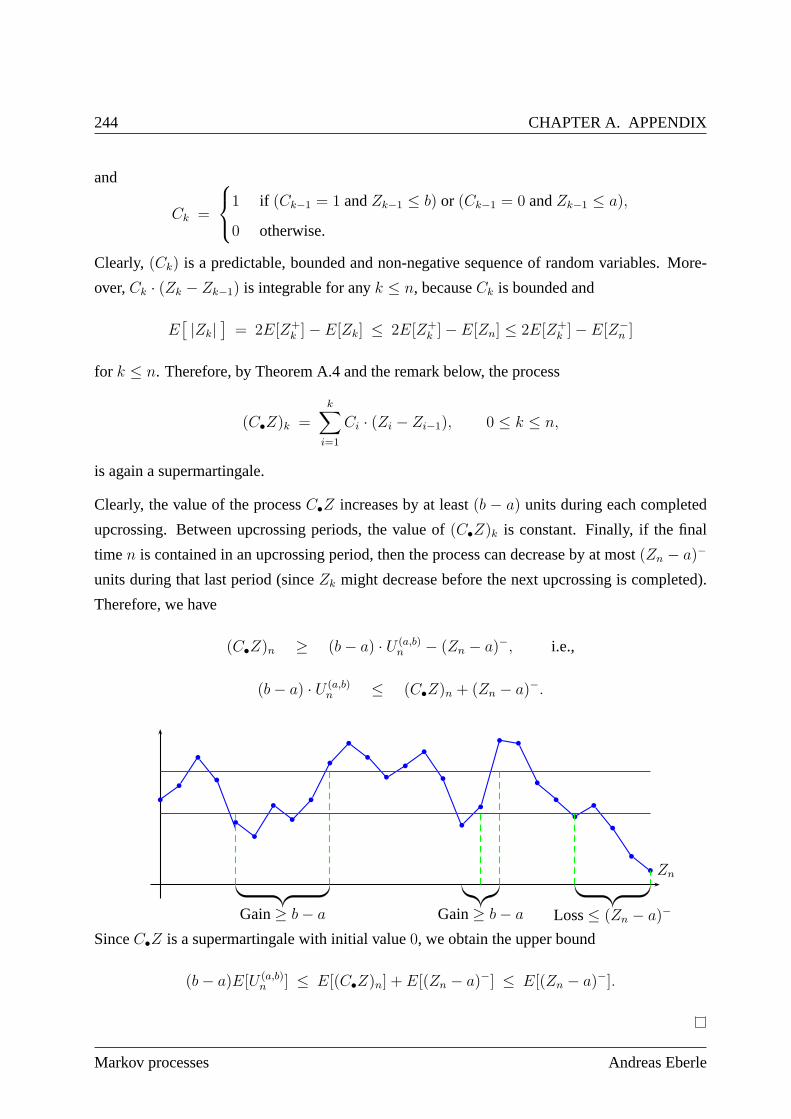
244 CHAPTER A. APPENDIX
and
Ck =
1 if (Ck−1 = 1 andZk−1 ≤ b) or (Ck−1 = 0 andZk−1 ≤ a),
0 otherwise.
Clearly, (Ck) is a predictable, bounded and non-negative sequence of random variables. More-
over,Ck · (Zk − Zk−1) is integrable for anyk ≤ n, becauseCk is bounded and
E[|Zk|
]= 2E[Z+
k ]− E[Zk] ≤ 2E[Z+k ]− E[Zn] ≤ 2E[Z+
k ]− E[Z−n ]
for k ≤ n. Therefore, by Theorem A.4 and the remark below, the process
(C•Z)k =k∑
i=1
Ci · (Zi − Zi−1), 0 ≤ k ≤ n,
is again a supermartingale.
Clearly, the value of the processC•Z increases by at least(b − a) units during each completed
upcrossing. Between upcrossing periods, the value of(C•Z)k is constant. Finally, if the final
timen is contained in an upcrossing period, then the process can decrease by at most(Zn − a)−
units during that last period (sinceZk might decrease before the next upcrossing is completed).
Therefore, we have
(C•Z)n ≥ (b− a) · U (a,b)n − (Zn − a)−, i.e.,
(b− a) · U (a,b)n ≤ (C•Z)n + (Zn − a)−.
Gain≥ b− a Gain≥ b− a Loss≤ (Zn − a)−
Zn
SinceC•Z is a supermartingale with initial value0, we obtain the upper bound
(b− a)E[U (a,b)n ] ≤ E[(C•Z)n] + E[(Zn − a)−] ≤ E[(Zn − a)−].
Markov processes Andreas Eberle
A.4. ALMOST SURE CONVERGENCE OF SUPERMARTINGALES 245
A.4.2 Proof of Doob’s Convergence Theorem
We can now complete the proof of Theorem A.8.
Proof. Let
U (a,b) = supn∈N
U (a,b)n
denote the total number of upcrossings of the supermartingale (Zn) over an interval(a, b) with
−∞ < a < b <∞. By the upcrossing inequality and monotone convergence,
E[U (a,b)] = limn→∞
E[U (a,b)n ] ≤ 1
b− a· supn∈N
E[(Zn − a)−]. (A.4.1)
AssumingsupE[Z−n ] < ∞, the right hand side of (A.4.1) is finite since(Zn − a)− ≤ |a| + Z−
n .
Therefore,
U (a,b) < ∞ P -almost surely,
and hence the event
lim inf Zn 6= lim supZn =⋃
a,b∈Qa<b
U (a,b) = ∞
has probability zero. This proves almost sure convergence.
It remains to show that the almost sure limitZ∞ = limZn is an integrable random variable
(in particular, it is finite almost surely). This holds true as, by the remark below Theorem A.8,
supE[Z−n ] <∞ implies that(Zn) is bounded inL1, and therefore
E[ |Z∞| ] = E[lim |Zn| ] ≤ lim inf E[ |Zn| ] < ∞
by Fatou’s lemma.
A.4.3 Examples and first applications
We now consider a few prototypic applications of the almost sure convergence theorem:
Example (Sums of i.i.d. random variables). Consider a Random Walk
Sn =n∑
i=1
ηi
onR with centered and bounded increments:
ηi i.i.d. with |ηi| ≤ c andE[ηi] = 0, c ∈ R.
University of Bonn Winter term 2014/2015
246 CHAPTER A. APPENDIX
Suppose thatP [ηi 6= 0] > 0. Then there existsε > 0 such thatP [|ηi| ≥ ε] > 0. As the
increments are i.i.d., the event|ηi| ≥ ε occurs infinitely often with probability one. Therefore,
almost surely the martingale(Sn) does not converge asn→ ∞.
Now leta ∈ R. We consider the first hitting time
Ta = minn ≥ 0 : Sn ≥ a
of the interval[a,∞). By the Optional Stopping Theorem, the stopped Random Walk(STa∧n)n≥0
is again a martingale. Moreover, asSk < a for anyk < Ta and the increments are bounded byc,
we obtain the upper bound
STa∧n < a+ c for anyn ∈ N.
Therefore, the stopped Random Walk converges almost surely by the Supermartingale Conver-
gence Theorem. As(Sn) does not converge, we can conclude thatP [Ta <∞] = 1 for anya > 0,
i.e.,
lim supSn = ∞ almost surely.
Since(Sn) is also a submartingale, we obtain
lim inf Sn = −∞ almost surely
by an analogue argument.
Remark (Almost sure vs.Lp convergence). In the last example, the stopped process does not
converge inLp for anyp ∈ [1,∞). In fact,
limn→∞
E[STa∧n] = E[STa ] ≥ a whereas E[S0] = 0.
Example (Products of non-negative i.i.d. random variables). Consider a growth process
Zn =n∏
i=1
Yi
with i.i.d. factorsYi ≥ 0 with finite expectationα ∈ (0,∞). Then
Mn = Zn/αn
is a martingale. By the almost sure convergence theorem, a finite limit M∞ exists almost surely,
becauseMn ≥ 0 for all n. For the almost sure asymptotics of(Zn), we distinguish three different
cases:
Markov processes Andreas Eberle
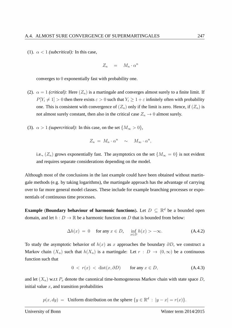
A.4. ALMOST SURE CONVERGENCE OF SUPERMARTINGALES 247
(1). α < 1 (subcritical): In this case,
Zn = Mn · αn
converges to0 exponentially fast with probability one.
(2). α = 1 (critical): Here(Zn) is a martingale and converges almost surely to a finite limit.If
P [Yi 6= 1] > 0 then there existsε > 0 such thatYi ≥ 1+ ε infinitely often with probability
one. This is consistent with convergence of(Zn) only if the limit is zero. Hence, if(Zn) is
not almost surely constant, then also in the critical caseZn → 0 almost surely.
(3). α > 1 (supercritical): In this case, on the setM∞ > 0,
Zn = Mn · αn ∼ M∞ · αn,
i.e., (Zn) grows exponentially fast. The asymptotics on the setM∞ = 0 is not evident
and requires separate considerations depending on the model.
Although most of the conclusions in the last example could have been obtained without martin-
gale methods (e.g. by taking logarithms), the martingale approach has the advantage of carrying
over to far more general model classes. These include for example branching processes or expo-
nentials of continuous time processes.
Example (Boundary behaviour of harmonic functions). Let D ⊆ Rd be a bounded open
domain, and leth : D → R be a harmonic function onD that is bounded from below:
∆h(x) = 0 for anyx ∈ D, infx∈D
h(x) > −∞. (A.4.2)
To study the asymptotic behavior ofh(x) asx approaches the boundary∂D, we construct a
Markov chain(Xn) such thath(Xn) is a martingale: Letr : D → (0,∞) be a continuous
function such that
0 < r(x) < dist(x, ∂D) for anyx ∈ D, (A.4.3)
and let(Xn) w.r.t Px denote the canonical time-homogeneous Markov chain with state spaceD,
initial valuex, and transition probabilities
p(x, dy) = Uniform distribution on the spherey ∈ Rd : |y − x| = r(x).
University of Bonn Winter term 2014/2015
248 CHAPTER A. APPENDIX
xr(x)
D
By (A.4.3), the functionh is integrable w.r.t.p(x, dy), and, by the mean value property,
(ph)(x) = h(x) for anyx ∈ D.
Therefore, the processh(Xn) is a martingale w.r.t.Px for eachx ∈ D. As h(Xn) is lower
bounded by (A.4.2), the limit asn → ∞ existsPx-almost surely by the Supermartingale Con-
vergence Theorem. In particular, since the coordinate functionsx 7→ xi are also harmonic and
lower bounded onD, the limitX∞ = limXn existsPx-almost surely. Moreover,X∞ is in ∂D,
becauser is bounded from below by a strictly positive constant on any compact subset ofD.
Summarizing we have shown:
(1). Boundary regularity: If h is harmonic and bounded from below onD then the limit
limn→∞
h(Xn) exists along almost every trajectoryXn to the boundary∂D.
(2). Representation ofh in terms of boundary values:If h is continuous onD, thenh(Xn) →h(X∞) Px-almost surely and hence
h(x) = limn→∞
Ex[h(Xn)] = E[h(X∞)],
i.e., the distribution ofX∞ w.r.t. Px is the harmonic measure on∂D.
Note that, in contrast to classical results from analysis, the first statement holds without any
smoothness condition on the boundary∂D. Thus, although boundary values ofh may not exist
in the classical sense, they still do exist along almost every trajectory of the Markov chain!
A.5 Brownian Motion
Definition (Brownian motion).
Markov processes Andreas Eberle
A.5. BROWNIAN MOTION 249
(1). Let a ∈ R. A continous-time stochastic processBt : Ω → R, t ≥ 0, definend on a
probability space(Ω,A, P ), is called aBrownian motion (starting in a)if and only if
a) B0(ω) = a for eachω ∈ Ω.
b) For any partition0 ≤ t0 ≤ t1 ≤ · · · ≤ tn, the incrementsBti+1− Bti are indepedent
random variables with distribution
Bti+1−Bti ∼ N(0, ti+1 − ti).
c) P -almost every sample patht 7→ Bt(ω) is continous.
d) AnRd-valued stochastic processBt(ω) = (B(1)t (ω), . . . , B
(d)t (ω)) is called a multi-dimensional
Brownian motion if and only if the component processes(B(1)t ), . . . , (B
(d)t ) are independent
one-dimensional Brownian motions.
Thus the increments of ad-dimensional Brownian motion are independent over disjointtime
intervals and have a multivariate normal distribution:
Bt −Bs ∼ N(0, (t− s) · Id) for any0 ≤ s ≤ t.
University of Bonn Winter term 2014/2015
Bibliography
[1] D. Bakry, I. Gentil, and M. Ledoux.AnalysisandGeometryof MarkovDiffusion Operators.
Grundlehren der mathematischen Wissenschaften. Springer, 2013.
[2] P. Billingsley. Convergenceof probabilitymeasures. Wiley Series in probability and Math-
ematical Statistics: Tracts on probability and statistics. Wiley, 1968.
[3] E. Bolthausen, A.S. Sznitman, and Deutschen Mathematiker-Vereinigung.TenLectureson
RandomMedia. DMV Seminar. Momenta, 2002.
[4] M. Chen. From Markov Chainsto Non-equilibriumParticleSystems. World Scientific,
2004.
[5] E.B. Davies.One-parametersemigroups. L.M.S. monographs. Academic Press, 1980.
[6] J.D. Deuschel and D.W. Stroock.Largedeviations. Pure and Applied Mathematics. Elsevier
Science, 1989.
[7] Andreas Eberle. Lecture „Introduction to Stochastic Analy-
sis“. Institute for Applied Mathematics, University of Bonn, 2011.
http://wt.iam.uni-bonn.de/fileadmin/WT/Inhalt/people/Andreas_Eberle/StoAn1011/StoAnSk
[8] Andreas Eberle. Lecture „Einführung in die Wahrscheinlichkeitstheo-
rie“. Institute for Applied Mathematics, University of Bonn, 2013.
http://wt.iam.uni-bonn.de/fileadmin/WT/Inhalt/people/Andreas_Eberle/Wtheorie13/Wtheor
[9] Andreas Eberle. Lecture „Stochastic Analysis“. Insti-
tute for Applied Mathematics, University of Bonn, 2013.
http://wt.iam.uni-bonn.de/fileadmin/WT/Inhalt/people/Andreas_Eberle/StoAn1213/Stochas
[10] Andreas Eberle. Lecture „Stochastic processes“. Insti-
tute for Applied Mathematics, University of Bonn, 2014.
http://wt.iam.uni-bonn.de/fileadmin/WT/Inhalt/people/Andreas_Eberle/StochProcesses/SP
250
BIBLIOGRAPHY 251
[11] S.N. Ethier and T.G. Kurtz.Markov processes:characterizationandconvergence. Wiley
series in probability and mathematical statistics. Probability and mathematical statistics.
Wiley, 1986.
[12] Martin Hairer. Lecture „Convergence of Markov pro-
cesses“. Mathematics Department, University of Warwick, 2010.
http://www.hairer.org/notes/Convergence.pdf.
[13] Galin L. Jones. On the markov chain central limit theorem. ProbabilitySurveys, 1:299–320,
2004.
[14] I. Karatzas and S.E. Shreve.BrownianMotion andStochasticCalculus. Graduate Texts in
Mathematics. Springer New York, 1991.
[15] R. Khasminskii. StochasticStability of Differential Equations. Stochastic Modelling and
Applied Probability. Springer, 2011.
[16] Claudio Landim. Central limit theorem for markov processes. In Pierre Picco and Jaime
San Martin, editors,From Classicalto Modern Probability, volume 54 ofProgressin
Probability, pages 145–205. Birkhaeuser Basel, 2003.
[17] S. Lang.AnalysisI. Addison-Wesley world student series. Addison-Wesley, 1978.
[18] T.M. Liggett. InteractingParticleSystems. Classics in Mathematics. Springer, 2004.
[19] T.M. Liggett. ContinuousTime Markov Processes:An Introduction. Graduate studies in
mathematics. American Mathematical Soc., 2010.
[20] Georg Lindgren. „Lecture notes on Stationary Stochastic Processes“. Lund In-
stitute of Technology Centre for Mathematical Sciences Mathematical Statistics, 2002.
http://www.maths.lth.se/matstat/staff/georg/Publications/lecture2002.pdf
[21] Florent Malrieu. Lecture „Processus de Markov et inégalités fonctionelles“, 2005/2006.
http://perso.univ-rennes1.fr/florent.malrieu/MASTER2/markov180406.pdf.
[22] Robert J. McCann. Exact solutions to the transportation problem on the line.R. Soc.Lond.
Proc.Ser.A Math.Phys.Eng.Sci., 455(1984):1341–1380, 1999.
[23] Sean Meyn and Richard L. Tweedie.Markov ChainsandStochasticStability. Cambridge
University Press, New York, NY, USA, 2nd edition, 2009.
University of Bonn Winter term 2014/2015
252 BIBLIOGRAPHY
[24] A. Pazy.Semigroupsof LinearOperatorsandApplicationsto PartialDifferentialEquations.
Applied Mathematical Sciences. Springer New York, 1992.
[25] S.T. Rachev and L. Rüschendorf.MassTransportationProblems:VolumeI: Theory. Mass
Transportation Problems. Springer, 1998.
[26] M. Reed and B. Simon.Methodsof modernmathematicalphysics.2. Fourier analysis,
self-adjointness. Fourier Nanlysis, Self-adjointness. Academic Press, 1975.
[27] M. Reed and B. Simon.Methodsof modernmathematicalphysics:Analysisof operators.
Methods of Modern Mathematical Physics. Academic Press, 1978.
[28] M. Reed and B. Simon.Methodsof ModernMathematicalPhysics:Functionalanalysis.
Number Bd. 1 in Methods of Modern Mathematical Physics. Academic Press, 1980.
[29] M. Reed and B. Simon.Methodsof Modern MathematicalPhysics: Scatteringtheory.
Number Bd. 3. Acad. Press, 1986.
[30] Gareth O. Roberts and Jeffrey S. Rosenthal. General statespace Markov chains and MCMC
algorithms.Probab.Surv., 1:20–71, 2004.
[31] L. C. G. Rogers and David Williams.Diffusions,Markov processes,andmartingales.Vol.
2. Cambridge Mathematical Library. Cambridge University Press, Cambridge, 2000. Itô
calculus, Reprint of the second (1994) edition.
[32] L.C.G. Rogers and D. Williams.Diffusions,Markov Processes,andMartingales:Volume
1, Foundations. Cambridge Mathematical Library. Cambridge University Press, 2000.
[33] G. Royer.An initiation to logarithmicSobolevinequalities. American Mathematical Soci-
ety, 2007.
[34] Daniel W. Stroock.c. Cambridge University Press, New York, NY, USA, 2nd edition, 2010.
[35] D.W. Stroock and S.R.S. Varadhan.MultidimensionalDiffussionProcesses. Grundlehren
der mathematischen Wissenschaften in Einzeldarstellungen mit besonderer Berücksichti-
gung der Anwendungsgebiete. Springer, 1979.
[36] S. R. S. Varadhan.ProbabilityTheory. Courant Lecture Notes. Courant Institute of Mathe-
matical Sciences, 2001.
Markov processes Andreas Eberle
BIBLIOGRAPHY 253
[37] C. Villani. Optimal Transport: Old and New. Grundlehren der mathematischen Wis-
senschaften. Springer, 2008.
[38] Cédric Villani. Topicsin OptimalTransportation. Graduate studies in mathematics. Amer-
ican Mathematical Society, 2003.
[39] K. Yosida. FunctionalAnalysis. Classics in Mathematics. Cambridge University Press,
1995.
University of Bonn Winter term 2014/2015