MANUAL: Materials and Mechanics Practice (PHY109P)

B. Tech: July---November 2017

IIITD&M Kancheepuram

Chennai – 600 127

LIST OF EXPERIMENTS:

CYCLE – I

1. TORSIONAL PENDULUM

2. BAR PENDULUM

3. CREEP TEST

4. TENSILE TEST

5. FRICTION

CYCLE – II

6. STRAIN GAUGE

7. THREE POINT BEND TEST

8. BUCKLING TEST

9. MICROSTRUCTURE

10. HARDNESS TEST AND

TORQUE MEASUREMNET

EX. NO.1: TORSIONAL PENDULUM

OBJECTIVE:

To find the modulus of rigidity (η) and torsional rigidity (C) of the given string.

APPARATUS REQUIRED:

Circular or rectangular discs suspended from a point using a metal wire about an axis passing through

the middle of plate having largest area, two similar weights, a stop watch and meter scale.

BRIEF DISCUSSION AND RELEVANT FORMULA:

For an object under torsion torsional, restoring torque is proportional to the angular displacements.

In practice, this will be true only for small angular displacements ‘θ’.

τ = 𝐼 𝑡𝑜𝑡 d2θ/dt2 = −C θ (1)

Again from Fig.2, we get the rigidity modulus

44

2 )(

r

l

r

rdFl

Lr

rdF

(2)

We can write the magnitude of C from (1) and (2), 𝐶 =𝜋 𝜂 𝑟4

2 𝑙 (3)

The equation gives the time period of torsional oscillations of the system as,

𝑇 = 2𝜋√ 𝐼 𝑡𝑜𝑡

𝐶 = 2𝜋√

𝐼 𝑜 + 2 𝐼 𝑠+ 2 m𝑠 𝑥2

𝐶 (4)

Io = moment of inertia of large disc (without any mass added to it) Is = moment of inertia of weight - about an axis passing through its/their own center of gravity, parallel to its/their length. ms = mass of each solid cylinder (weight)

x = distance of each weight from axis of suspension. C = torsional rigidity of suspension wire - (couple per unit twist).

Fig.1 Fig.2

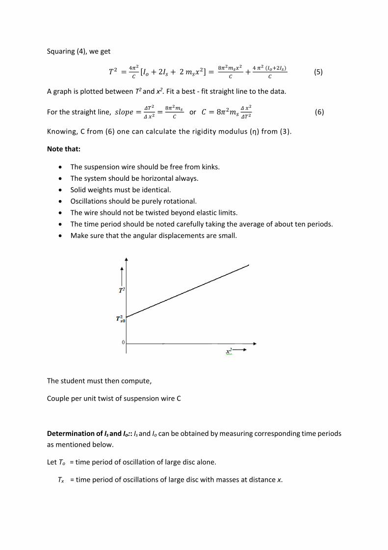
Squaring (4), we get

𝑇2 =4𝜋2

𝐶[𝐼𝑜 + 2𝐼𝑠 + 2 𝑚𝑠𝑥2] =

8𝜋2𝑚𝑠𝑥2

𝐶+

4 𝜋2 (𝐼𝑜+2𝐼𝑠)

𝐶 (5)

A graph is plotted between T2 and x2. Fit a best - fit straight line to the data.

For the straight line, 𝑠𝑙𝑜𝑝𝑒 =𝛥𝑇2

𝛥 𝑥2 =8𝜋2𝑚𝑠

𝐶 or 𝐶 = 8𝜋2𝑚𝑠

𝛥 𝑥2

𝛥𝑇2 (6)

Knowing, C from (6) one can calculate the rigidity modulus (η) from (3).

Note that:

The suspension wire should be free from kinks.

The system should be horizontal always.

Solid weights must be identical.

Oscillations should be purely rotational.

The wire should not be twisted beyond elastic limits.

The time period should be noted carefully taking the average of about ten periods.

Make sure that the angular displacements are small.

The student must then compute,

Couple per unit twist of suspension wire C

Determination of Is and Io:: Is and Io can be obtained by measuring corresponding time periods

as mentioned below.

Let To = time period of oscillation of large disc alone.

Tx = time period of oscillations of large disc with masses at distance x.

5

Tx0 = time period of oscillation of large disc with masses at x =0,(obtained from

graph – y intercept).

Putting these time periods in (5) , we will get a set of equations which will give us the following

expressions:

𝐼0 = 2𝑚𝑠𝑥2𝑇0

2

𝑇𝑥2 − 𝑇𝑥0

2 = 2𝑚𝑠𝑇0

2

𝑠𝑙𝑜𝑝𝑒

𝐼𝑠 = 𝑚𝑠𝑥2𝑇𝑥0

2 − 𝑇02

𝑇𝑥2 − 𝑇𝑥0

2 = 𝑚𝑠(𝑇𝑥0

2 − 𝑇02)

𝑠𝑙𝑜𝑝𝑒

OBSERVATIONS:

Mass of identical weights added, ms = ……………. kg

Time period of disc with no masses To = ……………….sec (averaged over 10 cycles)

Y-intercept from graph Txo = ………………sec

TABLE 1: MEASURE THE TIME PERIOD

Distance of weight

from axis of twist x

(cm)

x2

(cm2)

Number of

oscillations, n

Time taken

t (sec)

Period

T= t / n (sec)

T2

(sec2)

x1

x2

x3

x4

RESULT: 1. Rigidity modulus of the wire, η=

2. Couple per unit twist, C=

3. Moment of Inertia of the disc, Io=

6

EX.NO. 2: BAR PENDULUM

OBJECTIVE:

1. To determine the acceleration due to gravity (g) using a bar pendulum. 2. To verify that there are two pivot points on either side of the centre of gravity (C.G.)

about which the time period is the same. 3. To determine the radius of gyration of a bar pendulum by plotting a graph of time

period of oscillation against the distance of the point of suspension from C.G. 4. To determine the length of the equivalent simple pendulum.

APPARATUS REQUIRED:

Bar Pendulum, Small metal wedge, Spirit level, Stop watch, Meter rod THEORY:

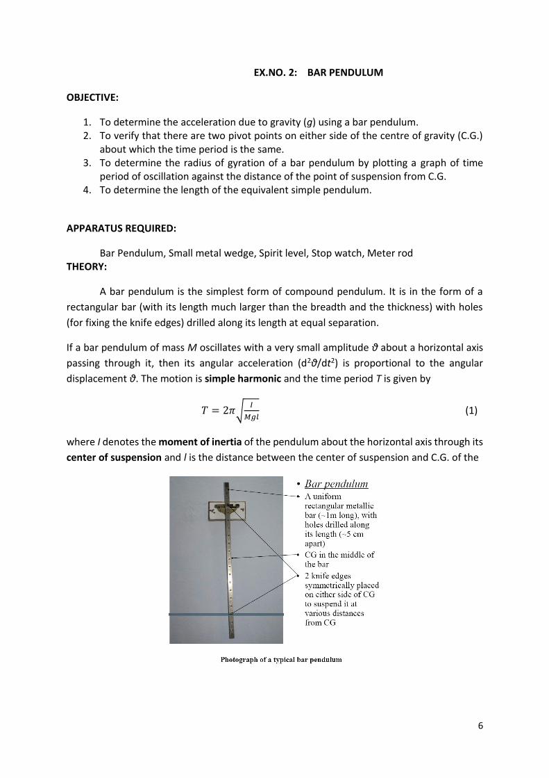
A bar pendulum is the simplest form of compound pendulum. It is in the form of a

rectangular bar (with its length much larger than the breadth and the thickness) with holes

(for fixing the knife edges) drilled along its length at equal separation.

If a bar pendulum of mass M oscillates with a very small amplitude θ about a horizontal axis

passing through it, then its angular acceleration (d2θ/dt2) is proportional to the angular

displacement θ. The motion is simple harmonic and the time period T is given by

𝑇 = 2𝜋√𝐼

𝑀𝑔𝑙 (1)

where I denotes the moment of inertia of the pendulum about the horizontal axis through its

center of suspension and l is the distance between the center of suspension and C.G. of the

7

Pendulum. According to the theorem of parallel axes, if IG is the moment of inertia of the

pendulum about an axis through C.G., then the moment of inertia I about a parallel axis at a

distance l from C.G. is given by

𝐼 = 𝐼𝐺 + 𝑀𝑙2

= 𝑀𝑘2 + 𝑀𝑙2 (2)

Where, k is the radius of gyration of the pendulum about the axis through C.G. Using Equation

(2) in Equation (1), we get 𝑇 = 2𝜋√𝑀k2+𝑀l2

𝑀𝑔𝑙

𝑇 = 2𝜋√k2+l2

𝑔𝑙 = 2𝜋√

𝑘2

𝑙⁄ +𝑙

𝑔 = 2𝜋√

𝐿

𝑔 (3)

Where, L is the length of the equivalent simple pendulum, given by

L = (𝑘2

𝑙⁄ + 𝑙) (4)

Therefore, from (1) and (4), g = 4π2 𝐿

𝑇2 (5)

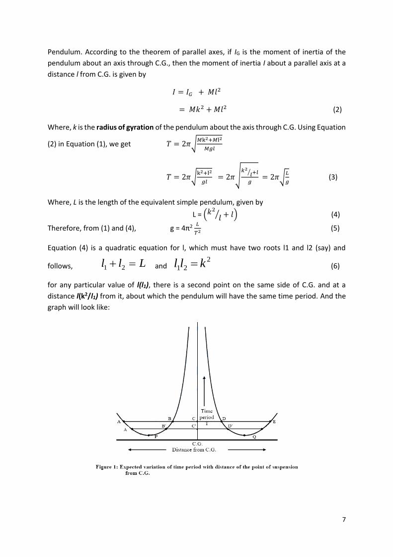
Equation (4) is a quadratic equation for l, which must have two roots l1 and l2 (say) and

follows, Lll 21 and 2

21 kll (6)

for any particular value of l(l1), there is a second point on the same side of C.G. and at a

distance l(k2/l1) from it, about which the pendulum will have the same time period. And the

graph will look like:

8

Ferguson’s method for determination of g Using Equations (4) and (5) we get

𝑙2 = 𝑔

4𝜋2𝑙𝑇2 − 𝑘2

A graph between 𝑙2 and 𝑙𝑇2 should therefore be a straight line with slope, 𝑔

4𝜋2 as shown in

(Figure2).

The intercept on the y-axis is –> k2.

Acceleration due to gravity, 𝑔 = 4𝜋2 × 𝑠𝑙𝑜𝑝𝑒

Radius of gyration, k =√(𝑖𝑛𝑡𝑒𝑟𝑐𝑒𝑝𝑡)

PROCEDURE:

1. Balance the bar on a sharp wedge and mark the position of its C.G. 2. Fix the knife edges in the outermost holes at either end of the bar pendulum. The knife

edges should be horizontal and lie symmetrically with respect to centre of gravity of the bar.

3. Check with spirit level that the glass plates fixed on the suspension wall bracket are horizontal. The support should be rigid.

4. Suspend the pendulum vertically by resting the knife edge at end A of the bar on the glass plate.

5. Displace the bar slightly to one side of the equilibrium position and let it oscillate with the amplitude not exceeding 5 degrees. Make sure that there is no air current in the vicinity of the pendulum.

6. Use the stop watch to measure the time for 20 oscillations. The time should be measured after the pendulum has had a few oscillations and the oscillations have become regular.

7. Measure the distance l from C.G. to the knife edge.

9

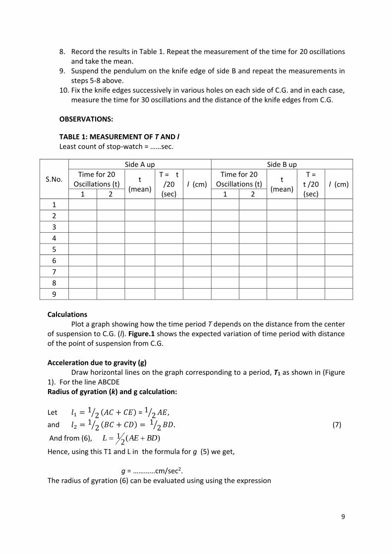
8. Record the results in Table 1. Repeat the measurement of the time for 20 oscillations and take the mean.

9. Suspend the pendulum on the knife edge of side B and repeat the measurements in steps 5-8 above.

10. Fix the knife edges successively in various holes on each side of C.G. and in each case, measure the time for 30 oscillations and the distance of the knife edges from C.G.

OBSERVATIONS:

TABLE 1: MEASUREMENT OF T AND l Least count of stop-watch = ……sec.

S.No.

Side A up Side B up

Time for 20 Oscillations (t)

t (mean)

T = t /20

(sec) l (cm)

Time for 20 Oscillations (t)

t (mean)

T = t /20 (sec)

l (cm) 1 2 1 2

1

2

3

4

5

6

7

8

9

Calculations

Plot a graph showing how the time period T depends on the distance from the center of suspension to C.G. (l). Figure.1 shows the expected variation of time period with distance of the point of suspension from C.G. Acceleration due to gravity (g)

Draw horizontal lines on the graph corresponding to a period, T1 as shown in (Figure 1). For the line ABCDE Radius of gyration (k) and g calculation:

Let 𝑙1 = 12⁄ (𝐴𝐶 + 𝐶𝐸) = 1 2⁄ 𝐴𝐸,

and 𝑙2 = 12⁄ (𝐵𝐶 + 𝐶𝐷) = 1

2⁄ 𝐵𝐷. (7)

And from (6), )(2

1 BDAEL

Hence, using this T1 and L in the formula for g (5) we get, g = ………...cm/sec2.

The radius of gyration (6) can be evaluated using using the expression

10

𝑘 = √𝑙1𝑙2 = ……….. cm.

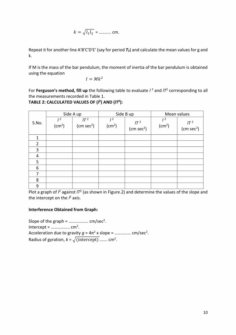
Repeat it for another line A'B'C'D'E' (say for period T2) and calculate the mean values for g and k. If M is the mass of the bar pendulum, the moment of inertia of the bar pendulum is obtained using the equation 𝐼 = 𝑀𝑘2 For Ferguson’s method, fill up the following table to evaluate l 2 and lT2 corresponding to all the measurements recorded in Table 1. TABLE 2: CALCULATED VALUES OF (l2) AND (lT2):

S.No.

Side A up Side B up Mean values

l 2 (cm2)

lT 2

(cm sec2)

l 2 (cm2)

lT 2

(cm sec2)

l 2 (cm2)

lT 2

(cm sec2)

1

2

3

4

5

6

7

8

9

Plot a graph of l2 against lT2 (as shown in Figure.2) and determine the values of the slope and the intercept on the l2 axis. Interference Obtained from Graph: Slope of the graph = ……………… cm/sec2. Intercept = …………….. cm2. Acceleration due to gravity g = 4π2 x slope = …………… cm/sec2.

Radius of gyration, k = √(intercept) ……. cm2.

11

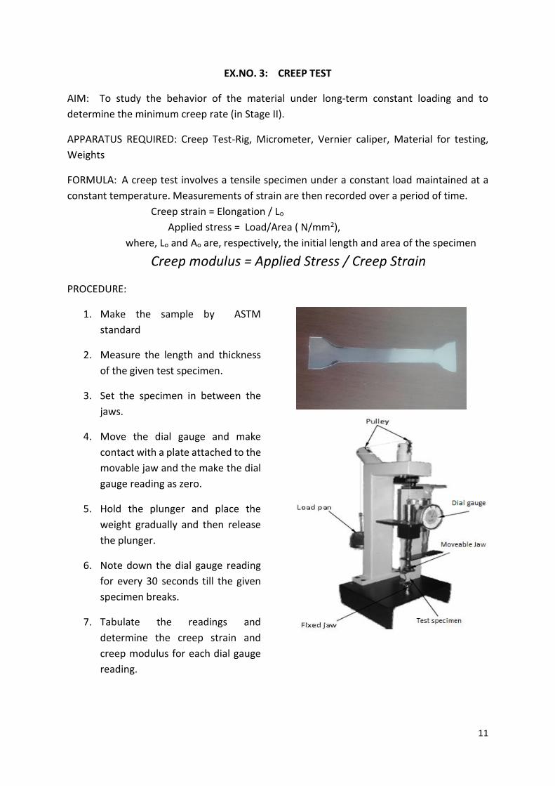
EX.NO. 3: CREEP TEST

AIM: To study the behavior of the material under long‐term constant loading and to

determine the minimum creep rate (in Stage II).

APPARATUS REQUIRED: Creep Test-Rig, Micrometer, Vernier caliper, Material for testing,

Weights

FORMULA: A creep test involves a tensile specimen under a constant load maintained at a

constant temperature. Measurements of strain are then recorded over a period of time.

Creep strain = Elongation / Lo

Applied stress = Load/Area ( N/mm2),

where, Lo and Ao are, respectively, the initial length and area of the specimen

Creep modulus = Applied Stress / Creep Strain

PROCEDURE:

1. Make the sample by ASTM

standard

2. Measure the length and thickness

of the given test specimen.

3. Set the specimen in between the

jaws.

4. Move the dial gauge and make

contact with a plate attached to the

movable jaw and the make the dial

gauge reading as zero.

5. Hold the plunger and place the

weight gradually and then release

the plunger.

6. Note down the dial gauge reading

for every 30 seconds till the given

specimen breaks.

7. Tabulate the readings and

determine the creep strain and

creep modulus for each dial gauge

reading.

TABLE 1: TO FIND THE CREEP MODULUS

Material Response for Stress (I) at 3.0 Kg:

S.NO TIME

(s)

ELONGATION

(mm)

CREEP

STRAIN

CREEP MODULUS

(N/mm2)

Repeat the same experiment with a different load for Stress(II) at 3.5kg.

13

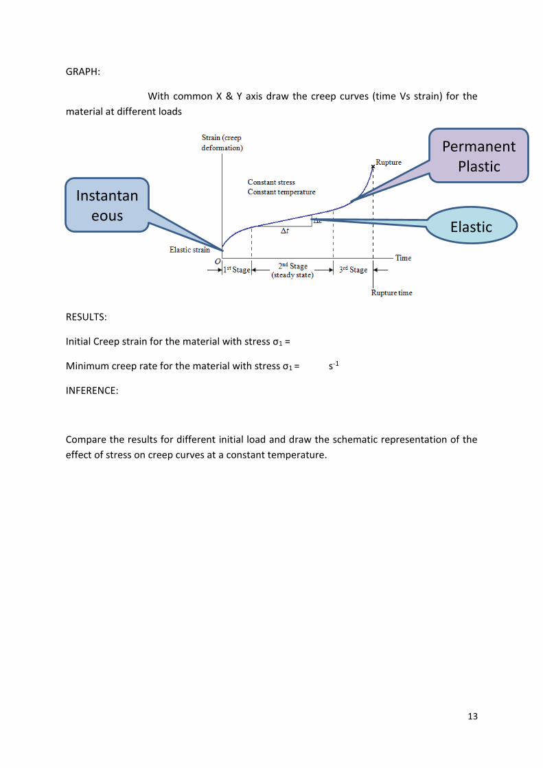
GRAPH:

With common X & Y axis draw the creep curves (time Vs strain) for the

material at different loads

RESULTS:

Initial Creep strain for the material with stress σ1 =

Minimum creep rate for the material with stress σ1 = s‐1

INFERENCE:

Compare the results for different initial load and draw the schematic representation of the

effect of stress on creep curves at a constant temperature.

Instantaneous

Elastic

Permanent Plastic Strain

Elastic Recove

14

EX. 4: TENSILE TEST

AIM: To study the response of the given specimens subjected to tensile load.

DESCRIPTION: The engineering tension test is widely used to provide basic design information

on the strength of the materials and as an accepted test for the specification of the materials.

In the tension test, a specimen is subjected to a continually increasing uniaxial tensile force

while simultaneous observations are made of the elongation of the specimen.

APPARATUS/ INSTRUMENT REQUIRED: INSTRON tensile testing machine, Capacity-2 kN,

Vernier caliper and scale, and Test specimens- As per ASTM standards

PROCEDURE:

1. Measure and record the initial dimension of the specimen (gauge length-L0, width w0,

thickness t0, cross section area Ao = w0× t0).

2. Fix the test specimen between fixed and movable jaws of the machine.

3. Reset the load to zero.

4. Operate the machine till the specimen fractures.

5. Measure and record the final configuration of the specimen (gauge length Lf, width wf,

thickness tf, cross section area Af = wf × tf).

6. Repeat the experiment for different strain rate (rate of loading).

7. Using the data acquired by the system, construct the stress-strain curves and find the

various parameters as listed in the calculation.

OBSERVATION:

Sl. No Material, Strain rate & Load Dimensions

(mm)

Fracture dimension

(mm)

1

Aluminium

Strain rate:

Load:

Lo= wo=

to= Ao =

Lf= wf=

tf= Af =

2

Nylon

Strain rate:

Load:

Lo= wo=

to= Ao =

Lf= wf=

tf= Af =

15

CALCULATIONS:

1. 2

0A mm

2. 2

fA mm

3. Ultimate tensile strength,

2max

0

/u

PS N mm

A

Where, Pmax is the maximum load

4. Yield strength, 2

0 /S N mm (obtain form graph)

Note: Yield strength is the stress required to produce a small specified amount of plastic

deformation. The usual definition of this property is the offset yield strength determined by

the stress corresponding to the intersection of the stress-strain curve and a line parallel to

the elastic part of the curve offset by a strain of 0.2%.

5. Breaking stress,

2

0

/f

f

PS N mm

A

where, fPis the breaking/fracture load (load at the occurrence of facture)

6. Strain,

0

0

f

f

L Le

L

7. Reduction in area at fracture,

0

0

fA Aq

A

8. Modulus of elasticity, E = Slope of initial linear portion of the curve, 2/N mm

9. Resilience,

220 /

2R

SU N mm

E

10. Toughness,

20 /2

uT f

S SU e N mm

PLOTS:

1. Engineering stress Vs Engineering strain

2. True stress Vs True strain

16

INFERENCE:

1. Compare the results and state which material has high strength, toughness, ductility,

and stiffness.

2. State the effect of strain rate in material response.

17

EX.5: DETERMINATION OF COEFFICIENT OF STATIC FRICTION

OBJECTIVE: To measure the static coefficient of friction for several combinations of material

surfaces.

APPARATUS REQUIRED: Inclined plane, Metal block, pull-push meter, set of weights and

materials with different surfaces.

FORMULA: Coefficient of static friction, 𝜇𝑆 = 𝑓𝑆

𝑁

Angle of static friction, 𝜑𝑠 = tan−1(𝜇𝑆)

where,

fS – Maximum static friction force (N)

N – Normal force applied (N)

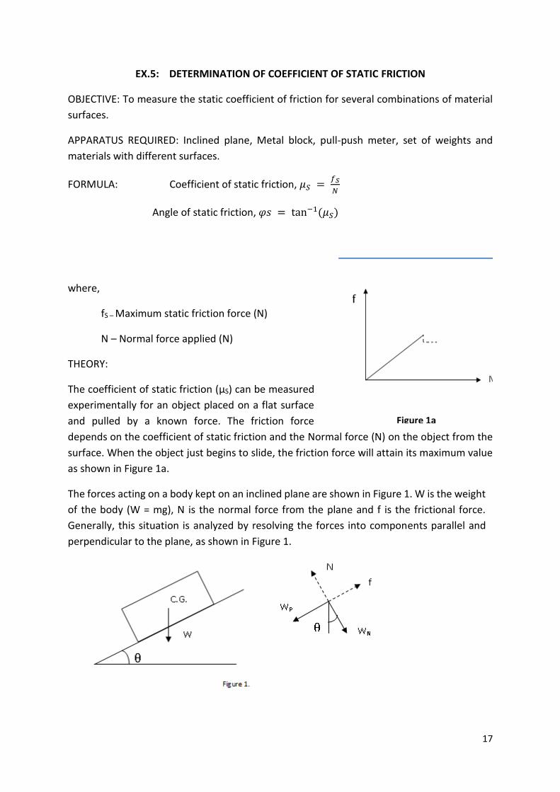
THEORY:

The coefficient of static friction (μS) can be measured

experimentally for an object placed on a flat surface

and pulled by a known force. The friction force

depends on the coefficient of static friction and the Normal force (N) on the object from the

surface. When the object just begins to slide, the friction force will attain its maximum value

as shown in Figure 1a.

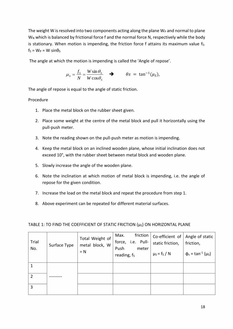
The forces acting on a body kept on an inclined plane are shown in Figure 1. W is the weight

of the body (W = mg), N is the normal force from the plane and f is the frictional force.

Generally, this situation is analyzed by resolving the forces into components parallel and

perpendicular to the plane, as shown in Figure 1.

Figure 1a

18

The weight W is resolved into two components acting along the plane WP and normal to plane

WN which is balanced by frictional force f and the normal force N, respectively while the body

is stationary. When motion is impending, the friction force f attains its maximum value fS.

fS = WP = W sinθS

The angle at which the motion is impending is called the ‘Angle of repose’.

S

SSS

W

W

N

f

cos

sin 𝜃𝑠 = tan−1(𝜇𝑆),

The angle of repose is equal to the angle of static friction.

Procedure

1. Place the metal block on the rubber sheet given.

2. Place some weight at the centre of the metal block and pull it horizontally using the

pull-push meter.

3. Note the reading shown on the pull-push meter as motion is impending.

4. Keep the metal block on an inclined wooden plane, whose initial inclination does not

exceed 10°, with the rubber sheet between metal block and wooden plane.

5. Slowly increase the angle of the wooden plane.

6. Note the inclination at which motion of metal block is impending, i.e. the angle of

repose for the given condition.

7. Increase the load on the metal block and repeat the procedure from step 1.

8. Above experiment can be repeated for different material surfaces.

TABLE 1: TO FIND THE COEFFICIENT OF STATIC FRICTION (μS) ON HORIZONTAL PLANE

Trial

No. Surface Type

Total Weight of

metal block, W

= N

Max. friction

force, i.e. Pull-

Push meter

reading, fS

Co-efficient of

static friction,

μS = fS / N

Angle of static

friction,

φs = tan-1 (μS)

1

---------

2

3

19

4

5

** Repeat this for other given surfaces also

TABLE 2: TO FIND THE COEFFICIENT OF STATIC FRICTION (μS) ON INCLINED PLANE

Trial

No. Surface Type Length (l) Height (h)

Angle of

repose, (𝜃𝑆)

𝜇𝑆=tan(𝜃𝑆)

1

--------

2

3

** Repeat this for other given surfaces

Graph

Plot a graph of the normal force (N) and the frictional force (fS) obtained while the metal block

was kept on the horizontal plane.

TABLE 3: Comparison of (i) values of μS, and (ii) the values of θS and φs.

Trail No. Surface Type

Angle of

Static

Friction

(𝜑𝑠)

Angle of

repose,

(𝜃𝑆)

μS (From Horizontal Plane)

μS ,

(From

Inclined

Plane)

20

EX. 6: YOUNG’S MODULUS OF WOOD USING A STRAIN GAUGE

AIM: To determine Young’s modulus of a half meter wooden scale using a Strain Gauge.

APPARATUS REQUIRED: A half meter scale with two identical strain gauges attached to one

end of the scale, one strain gauge at the top and the other at the bottom; another end of the

scale is attached to the table with a clamp; a circuit board with appropriate terminals to

constitute a Wheatstone bridge network.

STRAIN GAUGE:

Young’s modulus (Y) of the bar (scale) is defined by the ratio of stress (F/A) and tensile

strain(∆L/L),

𝐹/𝐴

∆L/L= Y … … … … … … … … … . . (1)

where, F is the force applied (Newton), A is the cross-sectional area (m2), ΔL is the

change in length (m), L is the original change in length (m).

A strain gauge is a transducer whose electrical resistance varies in proportional to the

amount of strain in the device. The most widely used gauge is metallic strain gauge which

consists of a very fine wire or, more commonly, metallic foil arranged in a grid pattern. The

grid pattern maximizes the amount of metallic wire or foil subject to strain in the parallel

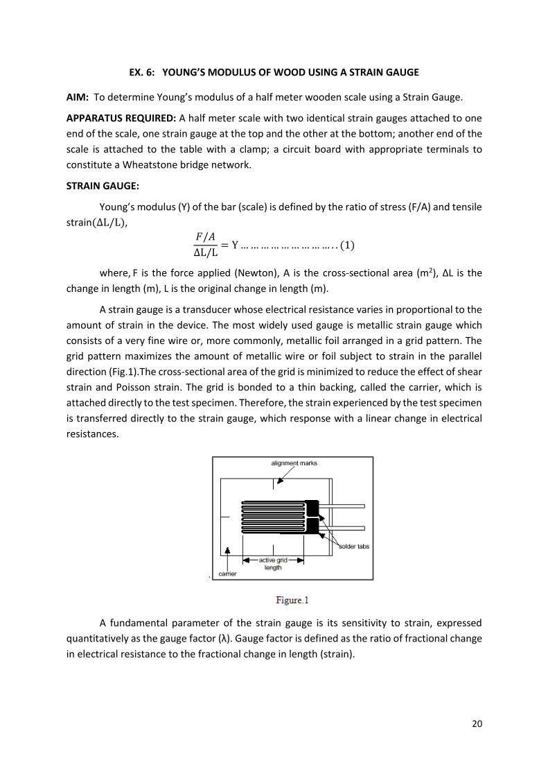
direction (Fig.1).The cross-sectional area of the grid is minimized to reduce the effect of shear

strain and Poisson strain. The grid is bonded to a thin backing, called the carrier, which is

attached directly to the test specimen. Therefore, the strain experienced by the test specimen

is transferred directly to the strain gauge, which response with a linear change in electrical

resistances.

A fundamental parameter of the strain gauge is its sensitivity to strain, expressed

quantitatively as the gauge factor (λ). Gauge factor is defined as the ratio of fractional change

in electrical resistance to the fractional change in length (strain).

21

∆𝑅/𝑅

∆𝐿/𝐿= 𝜆 … … … … … . … … … . . (2)

The gauge factor (λ) for metallic strain gauge is typically around 2.

WHEATSTONE BRIDGE:

Measuring the strain with a strain gauge requires accurate measurement of very small

change in resistance and such small changes in R can be measured with a Wheatstone bridge.

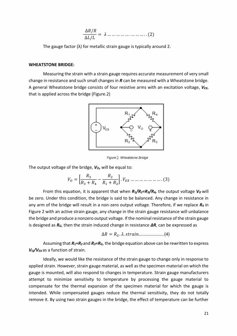
A general Wheatstone bridge consists of four resistive arms with an excitation voltage, VEX,

that is applied across the bridge (Figure.2)

The output voltage of the bridge, VO, will be equal to:

𝑉𝑂 = [𝑅3

𝑅3 + 𝑅4−

𝑅2

𝑅1 + 𝑅2] . 𝑉𝐸𝑋 … … … … … … … . (3)

From this equation, it is apparent that when R1/R2=R3/R4, the output voltage VO will

be zero. Under this condition, the bridge is said to be balanced. Any change in resistance in

any arm of the bridge will result in a non-zero output voltage. Therefore, if we replace R4 in

Figure 2 with an active strain gauge, any change in the strain gauge resistance will unbalance

the bridge and produce a nonzero output voltage. If the nominal resistance of the strain gauge

is designed as RG, then the strain induced change in resistance ∆R, can be expressed as

∆𝑅 = 𝑅𝐺 . 𝜆. 𝑠𝑡𝑟𝑎𝑖𝑛…………………..(4)

Assuming that R1=R2 and R3=RG, the bridge equation above can be rewritten to express

VO/VEX as a function of strain.

Ideally, we would like the resistance of the strain gauge to change only in response to

applied strain. However, strain gauge material, as well as the specimen material on which the

gauge is mounted, will also respond to changes in temperature. Strain gauge manufacturers

attempt to minimize sensitivity to temperature by processing the gauge material to

compensate for the thermal expansion of the specimen material for which the gauge is

intended. While compensated gauges reduce the thermal sensitivity, they do not totally

remove it. By using two strain gauges in the bridge, the effect of temperature can be further

22

minimized. For example, in a strain gauge configuration where one gauge is active (RG+∆R),

and a second gauge is placed transverse to the applied strain. Therefore, the strain has little

effect on the second gauge, called the dummy gauge. However, any changes in temperature

will affect both gauges in the same way. Because the temperature changes are identical in

the two gauges, the ratio of their resistance does not change, the voltage V0 does not change,

and the effects of the temperature change are minimized.

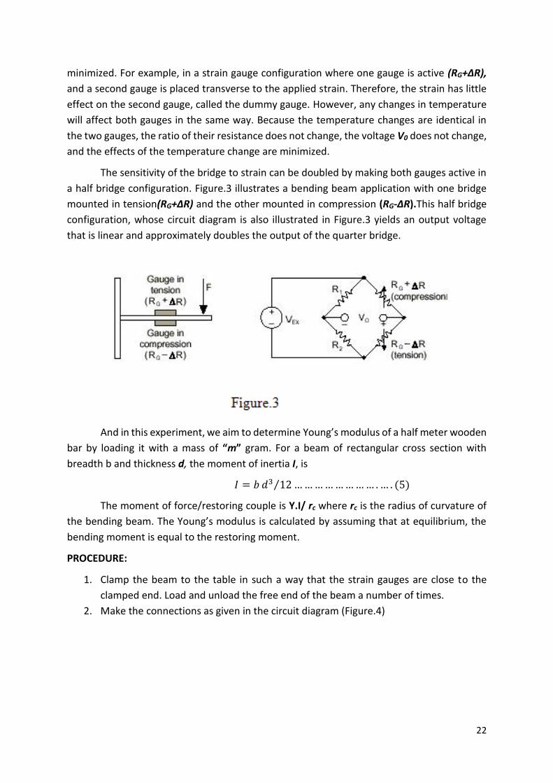
The sensitivity of the bridge to strain can be doubled by making both gauges active in

a half bridge configuration. Figure.3 illustrates a bending beam application with one bridge

mounted in tension(RG+∆R) and the other mounted in compression (RG-∆R).This half bridge

configuration, whose circuit diagram is also illustrated in Figure.3 yields an output voltage

that is linear and approximately doubles the output of the quarter bridge.

And in this experiment, we aim to determine Young’s modulus of a half meter wooden

bar by loading it with a mass of “m” gram. For a beam of rectangular cross section with

breadth b and thickness d, the moment of inertia I, is

𝐼 = 𝑏 𝑑3 12⁄ … … … … … … … … . … . (5)

The moment of force/restoring couple is Y.I/ rc where rc is the radius of curvature of

the bending beam. The Young’s modulus is calculated by assuming that at equilibrium, the

bending moment is equal to the restoring moment.

PROCEDURE:

1. Clamp the beam to the table in such a way that the strain gauges are close to the

clamped end. Load and unload the free end of the beam a number of times.

2. Make the connections as given in the circuit diagram (Figure.4)

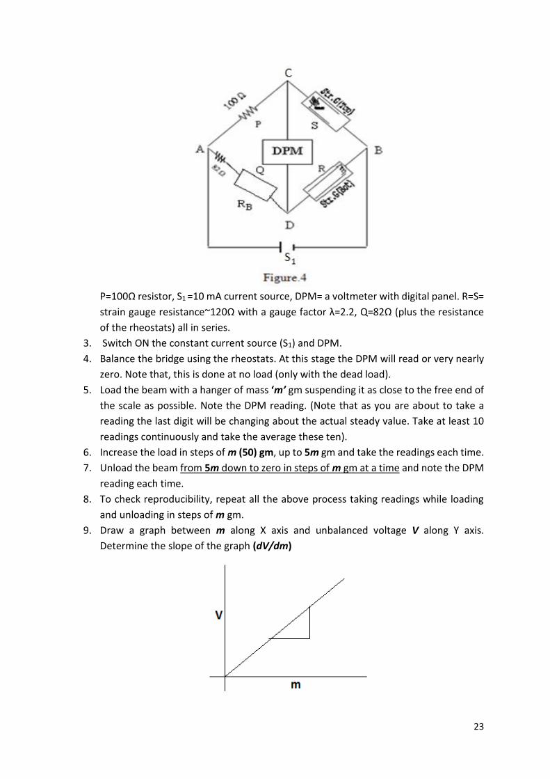
23

P=100Ω resistor, S1 =10 mA current source, DPM= a voltmeter with digital panel. R=S=

strain gauge resistance~120Ω with a gauge factor λ=2.2, Q=82Ω (plus the resistance

of the rheostats) all in series.

3. Switch ON the constant current source (S1) and DPM.

4. Balance the bridge using the rheostats. At this stage the DPM will read or very nearly

zero. Note that, this is done at no load (only with the dead load).

5. Load the beam with a hanger of mass ‘m’ gm suspending it as close to the free end of

the scale as possible. Note the DPM reading. (Note that as you are about to take a

reading the last digit will be changing about the actual steady value. Take at least 10

readings continuously and take the average these ten).

6. Increase the load in steps of m (50) gm, up to 5m gm and take the readings each time.

7. Unload the beam from 5m down to zero in steps of m gm at a time and note the DPM

reading each time.

8. To check reproducibility, repeat all the above process taking readings while loading

and unloading in steps of m gm.

9. Draw a graph between m along X axis and unbalanced voltage V along Y axis.

Determine the slope of the graph (dV/dm)

24

10. Note the distance between the center of the strain gauges and the point of application

of the load (L).

11. Measure the breadth of the beam using slide calipers (b).

12. Measure the thickness of the beam using a screw gauge (d).

13. Young’s modulus of the material of the beam, which is nothing but stress to strain

ratio, is given by the following expression (Working formula).

𝑌 =6𝑔𝐿𝜆𝑅𝐼

𝑏𝑑2[1 + (𝑅 𝑃⁄ )]𝑑𝑉𝑑𝑚

… … … … … … … … . (5)

where

o g is the acceleration due to gravity,

o λ is the gauge factor (for metal strain gauge λ =2.2).

o I is the output current from the source S1.

o R is the resistance of strain gauge.

o 𝑑𝑉

𝑑𝑚 is slope of the m Vs V curve

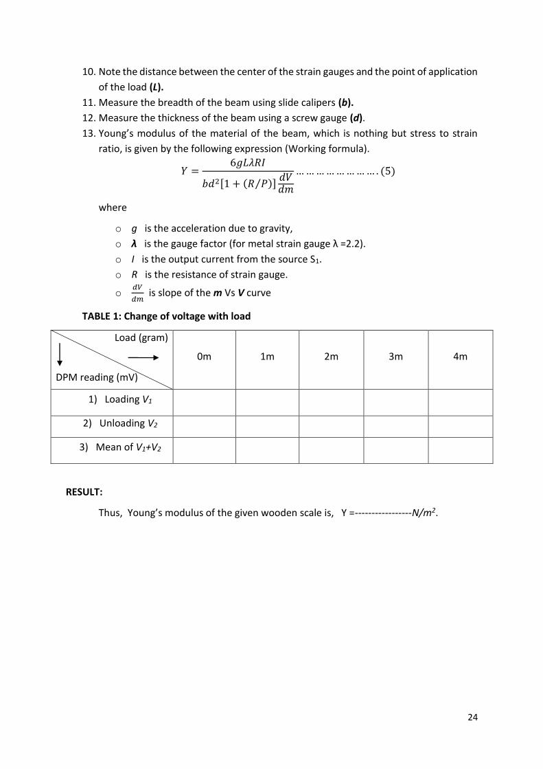
TABLE 1: Change of voltage with load

Load (gram)

DPM reading (mV)

0m 1m 2m 3m 4m

1) Loading V1

2) Unloading V2

3) Mean of V1+V2

RESULT:

Thus, Young’s modulus of the given wooden scale is, Y =-----------------N/m2.

25

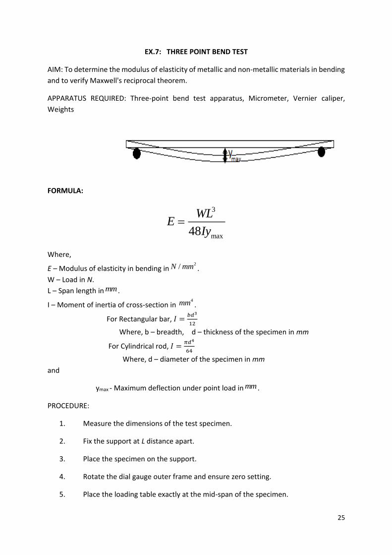
EX.7: THREE POINT BEND TEST

AIM: To determine the modulus of elasticity of metallic and non‐metallic materials in bending

and to verify Maxwell's reciprocal theorem.

APPARATUS REQUIRED: Three-point bend test apparatus, Micrometer, Vernier caliper,

Weights

FORMULA:

3

max48

WLE

Iy

Where,

E – Modulus of elasticity in bending in2/N mm .

W – Load in N.

L – Span length in mm .

I – Moment of inertia of cross-section in 4mm .

For Rectangular bar, 𝐼 =𝑏𝑑3

12

Where, b – breadth, d – thickness of the specimen in mm

For Cylindrical rod, 𝐼 =𝜋𝑑4

64

Where, d – diameter of the specimen in mm

and

ymax - Maximum deflection under point load in mm .

PROCEDURE:

1. Measure the dimensions of the test specimen.

2. Fix the support at L distance apart.

3. Place the specimen on the support.

4. Rotate the dial gauge outer frame and ensure zero setting.

5. Place the loading table exactly at the mid-span of the specimen.

26

6. Place the weight on the loading pan and note down the total load and deflection

from the dial gauge.

7. Increase the load in steps and measure the deflection.

8. Vary the span length and repeat the experiment for each specimen.

9. Calculate the modulus of elasticity in bending.

10. Repeat the experiment for different specimens.

OBSERVATION:

TABLE 1: TO FIND THE BREADTH OF THE SPECIMEN: LC= __________

S. No MSR

(mm)

VSC

(div)

VSR = (VSC*LC)

(mm)

TR = MSR+VSR

(mm)

Mean

TABLE 2: TO FIND THE THICKNESS OF THE SPECIMEN : LC= __________

S.

No

MSR

(mm)

VSC

(div)

VSR = (VSC*LC)

(mm)

TR = MSR+VSR

(mm)

Mean

27

TABLE 3: TO FIND THE DIAMETER OF THE SPECIMEN USIND SCREW GAUGE: LC= ______

S. No PSR

(mm)

HSC

(div)

HSR = (VSC*LC)

(mm)

TR = PSR+HSR

(mm)

CR= TR±ZE (mm)

Mean

TABLE 4: TO FIND THE MODULUS OF ELASTICITY FOR DIFFERENT MATERAILS

Span Length

(mm)

Load

(N)

Deflection

(mm)

Modulus of elasticity

in bending (N/mm2)

Avg. Modulus of elasticity

in bending (N/mm2)

Specimen-1:____________

Moment of Inertia, I=

Specimen-2:

Moment of Inertia, I=

28

Specimen-3:

Moment of Inertia, I=

CALCULATIONS: Use formulae ---

𝑰 =𝒃𝒅𝟑

𝟏𝟐 𝑰 =

𝝅𝒅𝟒

𝟔𝟒

3

max48

WLE

Iy

GRAPH: Draw the graph of load(P) vs deflection(y) for different specimens using common

X & Y axis.

M1, M2 and M3 are different

materials

deflection

Load

M1

M3

M2

29

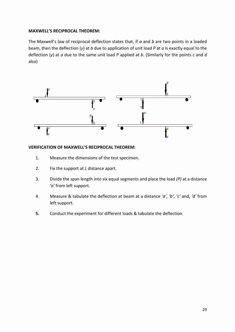
MAXWELL’S RECIPROCAL THEOREM:

The Maxwell’s law of reciprocal deflection states that, if a and b are two points in a loaded

beam, then the deflection (y) at b due to application of unit load P at a is exactly equal to the

deflection (y) at a due to the same unit load P applied at b. (Similarly for the points c and d

also)

VERIFICATION OF MAXWELL’S RECIPROCAL THEOREM:

1. Measure the dimensions of the test specimen.

2. Fix the support at L distance apart.

3. Divide the span length into six equal segments and place the load (P) at a distance

‘a’ from left support.

4. Measure & tabulate the deflection at beam at a distance ‘a’, ‘b’, ‘c’ and, ‘d’ from

left support.

5. Conduct the experiment for different loads & tabulate the deflection.

30

TABLE 5: VERIFICATION MAXWELL’S RECIPROCAL THEOREM

Specimen:

Dimension:

l = ------; b = -------; t = -------

Span length:

Load location

(from left

support)

Load

Deflection

a c b d

a

c

b

d

Repeat this TABLE for different materials with different dimensions.

INFERENCES:

1. State the reason for variation in Eavg value in different span length

2. State how the cross section of the beam affects the deflection

31

EX.08: BUCKLING OF COLUMNS EXPERIMENT

OBJECTIVE: To observe the buckling behavior of columns and estimate their buckling loads

for different end conditions

APPARATUS REQUIRED: Structural testing frame set-up, columns made of different materials,

weights, traveling microscope, vernier calipers and screw gauge.

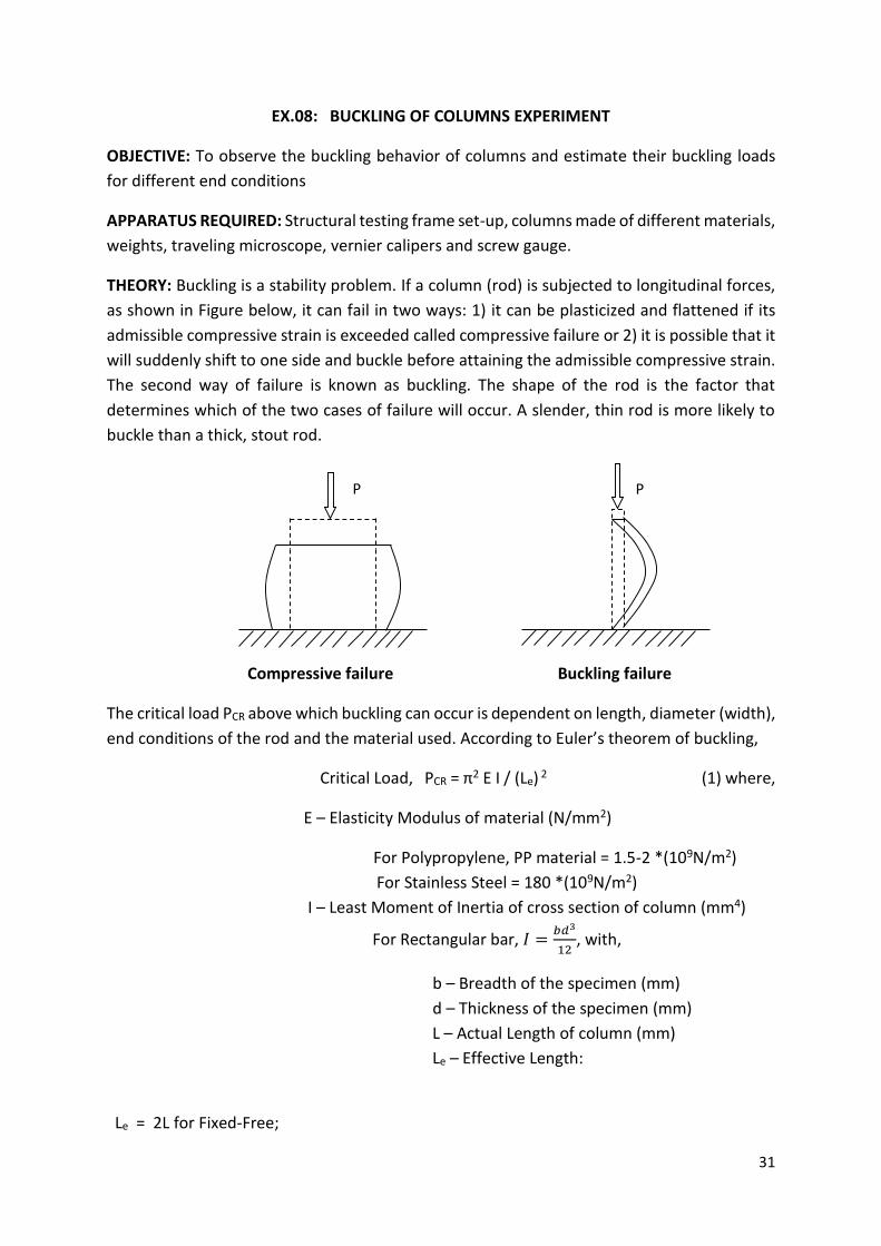
THEORY: Buckling is a stability problem. If a column (rod) is subjected to longitudinal forces,

as shown in Figure below, it can fail in two ways: 1) it can be plasticized and flattened if its

admissible compressive strain is exceeded called compressive failure or 2) it is possible that it

will suddenly shift to one side and buckle before attaining the admissible compressive strain.

The second way of failure is known as buckling. The shape of the rod is the factor that

determines which of the two cases of failure will occur. A slender, thin rod is more likely to

buckle than a thick, stout rod.

Compressive failure Buckling failure

The critical load PCR above which buckling can occur is dependent on length, diameter (width),

end conditions of the rod and the material used. According to Euler’s theorem of buckling,

Critical Load, PCR = π2 E I / (Le) 2 (1) where,

E – Elasticity Modulus of material (N/mm2)

For Polypropylene, PP material = 1.5-2 *(109N/m2)

For Stainless Steel = 180 *(109N/m2)

I – Least Moment of Inertia of cross section of column (mm4)

For Rectangular bar, 𝐼 =𝑏𝑑3

12, with,

b – Breadth of the specimen (mm)

d – Thickness of the specimen (mm)

L – Actual Length of column (mm)

Le – Effective Length:

Le = 2L for Fixed-Free;

P P

32

= 1.0 L for both Pinned

= 0.7 L for Fixed-Pinned

= 0.5 L for both Fixed.

Fixed-Free Both pinned Fixed-Pinned Both fixed

Euler derived the equation (1) for columns with no consideration for lateral forces. However,

if lateral forces are taken into consideration the value of critical load remains approximately

the same. In deriving equation (1), initial lateral deflection of the column has also been taken

zero. If the initial deflection of the mid point of the column is ‘a’ and instantaneous mid point

deflection is δ, then the critical load can be expressed in terms of its load and deflection of

mid-point as (Southwell plot);

(2)

PROCEDURE

CRCRCR P

a

PPP

P

a

1

1

33

1. Measure the length, breadth, and thickness of the column which is to be used in the

experiment.

2. Note the Elasticity Modulus of the material given to you.

3. Mount the column providing the required end condition (You may use fixed-free end

condition at first).

4. Focus the telescope on the column.

5. Gradually apply a load in small steps on the column using weights on top of the frame

set-up and note down the load and the corresponding lateral deflection of the column

using dial gauge.

6. Continue step 4 till the lateral deflection is noticeable, i.e. column is no longer straight,

and then remove the load.

7. Change the end condition to fixed-fixed, pinned-pinned, pinned-fixed, and repeat the

experiment from step 3.

8. Repeat the experiment with columns made of different materials and different cross

sections.

TABLE-1: Measurement of deflection with a change in load.

MATERIAL:

Sl.No End

conditions

Length of

column (mm)

Applied Load,

P (kgf)

Lateral

Deflection, δ

(mm)

Ratio

δ/P,

(mm/kgf)

Fixed-Fixed

Fixed-Pinned

34

Pinned-

Pinned

Repeat this experiment with different material.

Table-2: TO FIND THE BREADTH OF THE SPECIMEN: LC= __________

S. No MSR

(mm)

VSC

(div)

VSR = (VSC*LC)

(mm)

TR = MSR+VSR

(mm)

Mean

Table-3: TO FIND THE THICKNESS OF THE SPECIMEN: LC= __________

S.

No

MSR

(mm)

VSC

(div)

VSR = (VSC*LC)

(mm)

TR = MSR+VSR

(mm)

Mean

*Plot a graph between the measured lateral deflection (abscissa) and the ratio (δ/P). The

inverse of the slope of the curve gives the experimental critical load (using Data from Table1).

35

TABLE 4: ERROR calculation.

Caution:

DO NOT overload the column beyond the critical value (and/or DO NOT attempt for high

lateral deflections) as it may result in permanent plastic deformation to the column and/or

breaking of columns.

RESULT/conclusion: for example remark about theoretical and experimental values of PCR.

Sl.No End

conditions

Length of

column

(mm)

Effective length

of column(mm)

Theoretical

Critical

Load, PCR

(N)

Experimental

Critical Load

PCR (N)

Error

(%)

36

EX.9: MICROSTRUCTURE PRACTICE

OBJECTIVE: To see and study the microstructure for cast iron and steel 304.

APPARATUS REQUIRED: Sample, Grinding machine, Emery sheets with different grades,

Metallurgical Inverted Microscope, Polishing machine, Alumina powder, Etchant, Cotton.

THEORY: Internal structure of a material is viewed on a Microscopic scale. Microstructure

refers to the fine surface structure of a pure metal or alloy, as revealed by magnifications of

25X or greater.

The microstructure of a material (such as metals, polymers, ceramics or composites) can

strongly influence physical properties such as strength, toughness, ductility, hardness,

corrosion resistance, high/low-temperature behavior or wear resistance.

PROCEDURE:

Steps: - Moulding

1. Make the given material into small pieces for testing

2. Prepare the molding to hold the sample.

Moulding Preparation: Mix the cold setting compounds into a colloidal form, use both liquid

and powder in a proper mixture.

3. Place the small piece of test material at the bottom of the mould ring, and then pour

the prepared colloidal mixture on it.

4. Leave that for 15 – 20 minutes to get harden moulding

5. The sample is ready for the test procedure.

37

Steps: - Testing

1. Remove the roughness and micro burs of the sample with the help of belt grinding

machine

2. Polish the sample with various grades of emery sheet like 320, 400, 600, 800 and

higher grit abrasives, until the desired finish is achieved.

3. Use the alumina powder on disc polishing machine, to get the smooth and impressive

surface on the sample.

4. Clean the specimen with cotton

5. Apply the etchant – NITAL (98% Ethanol & 2% Nitric acid)

6. Check the microstructure and draw the structure you see for each sample and comment

on it.

Fig: Sample work piece to view microstructure

Fig.1 – Mild Steel Fig.2 – Cast Iron

Grains

Grain

Boundary

38

EX.10a: TORQUE MEASUREMENTS

OBJECTIVE: To understand the working principle of strain gauge and to measure the torque

using strain gauge

APPARATUS REQUIRED: Torque measurement kit with digital indicator, Weights, Meter Scale

FORMULA:

τ = r × F (1)

where

τ – Torque measured (kg-m)

r – radius from the origin point (m)

F – force applied (kg)

PROCEDURE: TORQUE MEASUREMENT

1. Switch on the instrument.

2. Using coarse and fine adjusting knobs set the reading in to zero.

3. Place the weight on the load pan and note down the torque values for a particular

length.

4. Note down the readings during successive loading and unloading and take the average

value for the particular load.

5. Repeat this for other length values.

6. Compare the strain gauge readings with theoretical torque.

TABLE 1: Variation of torque with load.

39

S.NO

TORQUE

ARM

LENGTH

(m)

LOAD

(g)

STRAIN GAUGE READING (kg-m) THEORETICAL

TORQUE

(kg-m) LOADING UNLOADING AVERAGE

1 1

2 0.75

3 0.5

4 0.25

40

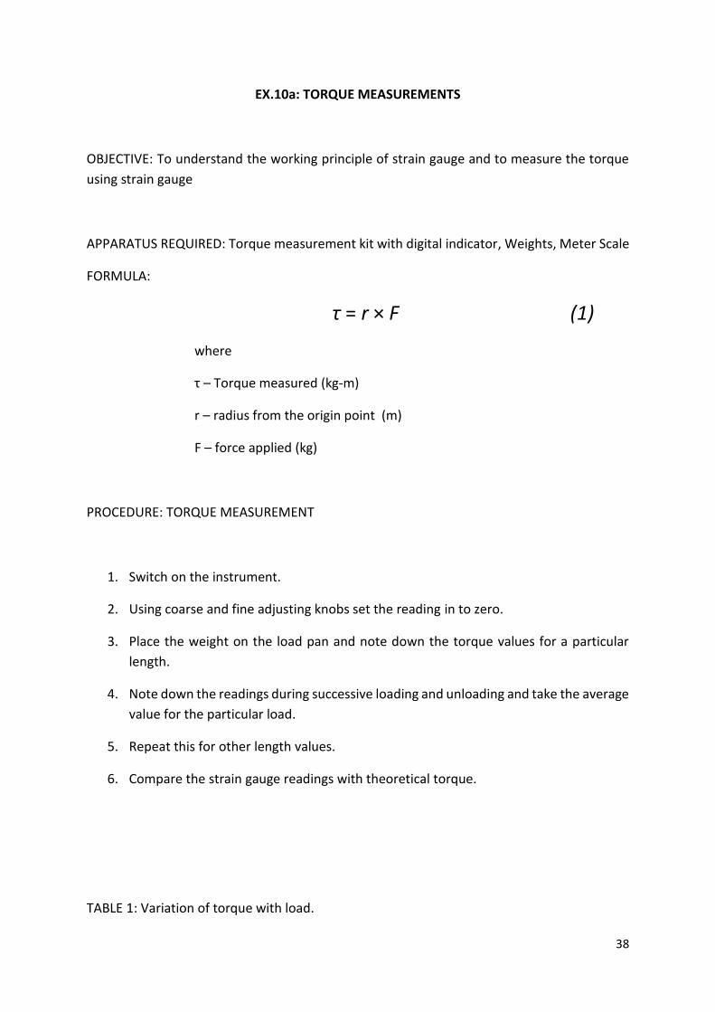
GRAPH:

Plot the graph of Load Vs Strain gauge measured torque & theoretical torque on

common X & Y axis graph.

RESULT:

The working principle of the strain gauge is understood through measuring strain and torque

using the strain gauge in a Wheatstone bridge circuit.

INFERENCE:

As for example “State the reason for the variation in theoretical & experimental strain &

torque values.”

Torq

ue

valu

e

Load

Strain gauge

Theoretical Measureme

41

EX.10b: HARDNESS TEST

OBJECTIVE: To find the Hardness number of different materials

APPARATUS REQUIRED: Digital Rockwell Hardness Test Machine, Indenters like Diamond tip

and steel ball with various diameters, Different materials for testing

THEORY: Hardness refers to various properties of matter in the solid phase that gives it high

resistance to various kinds of shape change when force is applied. The hard matter is

contrasted with the matter. Macroscopic hardness is generally characterized by strong

intermolecular bonds. However, the behavior of solid materials under force is complex,

resulting in several different scientific definitions of what might be called "hardness" in

everyday usage.

In materials science, there are three principal operational definitions of hardness:

Scratch hardness: Resistance to fracture or plastic (permanent) deformation

due to friction from a sharp object

Rebound hardness: Height of the bounce of an object dropped on the

material, related to elasticity.

Indentation hardness: Resistance to plastic (permanent) deformation due to

a constant load from a sharp object

The equation based definition of hardness is the pressure applied over the projected contact

area between the indenter and the material being tested. As a result hardness values are

typically reported in units of pressure, although this is only a "true" pressure if the indenter

and surface interface is perfectly flat.

The Rockwell scale is a hardness scale based on the indentation hardness of a material. The

Rockwell test determines the hardness by measuring the depth of penetration of an indenter

under a large load compared to the penetration made by a preload. There are different

scales, which are denoted by a single letter (say X), that use different loads or indenters. The

result, which is a dimensionless number, is noted by HRX where X is the scale letter.

The Hardness number is, = HR X (NUMBER). Where,

HR – Rockwell Hardness, X – Scale corresponds, Number–numerical digit for the

particular material

When testing metals, indentation hardness correlates linearly with tensile strength. This

important relation permits economically important non-destructive testing of bulk metal

42

deliveries with lightweight, even portable equipment, such as hand-held Rockwell hardness

testers.

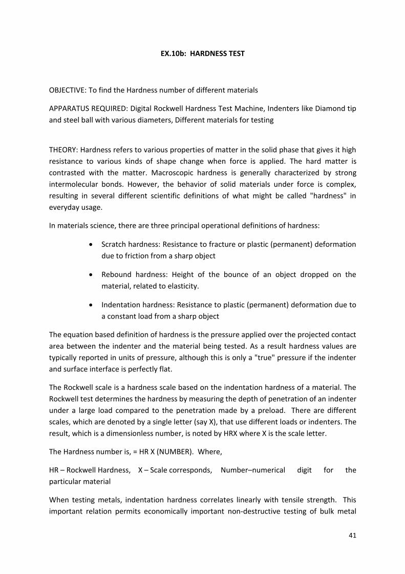
Rockwell Hardness Test

Fig.1 Hardness testing machine Fig.2 Hardness testing process

The Rockwell hardness test method consists of indenting the test material with a diamond

cone or hardened steel ball indenter. The indenter is forced into the test material under a

preliminary minor load F0 (Fig. 2a) usually 10 kg. When equilibrium is reached, an indicating

device, which follows the movements of the indenter and so responds to changes in depth of

penetration of the indenter, is set to a datum position. While the preliminary minor load is

still applied, an additional major load is applied resulting an increase in penetration (Fig. 2b).

When equilibrium is reached, the additional major load is removed but the preliminary minor

load is still maintained. Removal of the additional major load allows a partial recovery, so

reducing the depth of penetration (Fig.2c). The permanent increase in depth of penetration,

resulting from the application and removal of the additional major load is used to calculate

the Rockwell hardness number.

HR = E - e

F0 = preliminary minor load in kgf

F1 = additional major load in kgf

F = total load in kgf

e = permanent increase in depth of penetration due to major load F1 measured in units of

0.002 mm

43

E = a constant depending on form of indenter: 100 units for diamond indenter, 130 units for

steel ball indenter

HR = Rockwell hardness number

D = diameter of steel ball

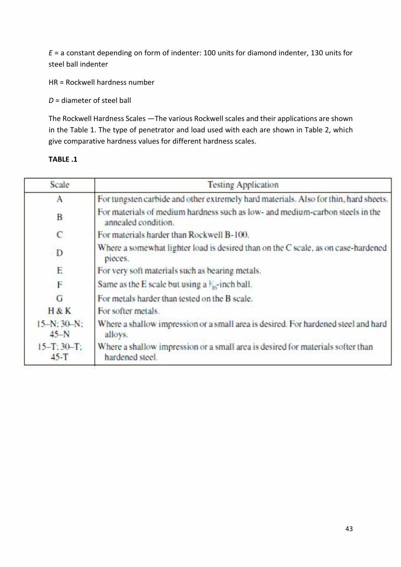
The Rockwell Hardness Scales —The various Rockwell scales and their applications are shown

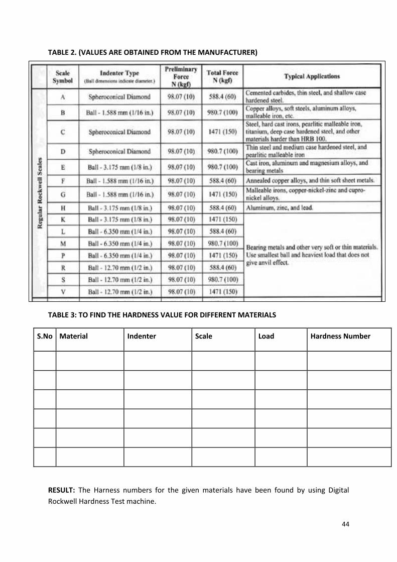
in the Table 1. The type of penetrator and load used with each are shown in Table 2, which

give comparative hardness values for different hardness scales.

TABLE .1

44

TABLE 2. (VALUES ARE OBTAINED FROM THE MANUFACTURER)

TABLE 3: TO FIND THE HARDNESS VALUE FOR DIFFERENT MATERIALS

S.No Material Indenter Scale Load Hardness Number

RESULT: The Harness numbers for the given materials have been found by using Digital

Rockwell Hardness Test machine.

45