Macromechanics of a Laminate

Textbook: Mechanics of Composite Materials Author: Autar Kaw

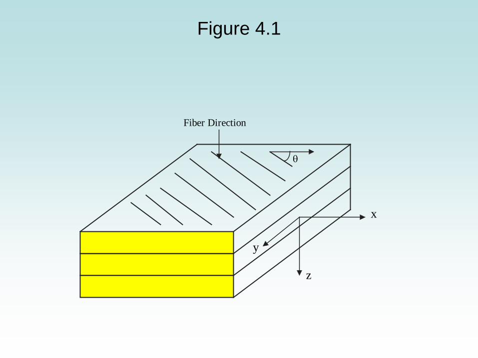
Figure 4.1

Fiber Direction

θ

x

z

y

CHAPTER OBJECTIVES

Understand the code for laminate stacking sequence Develop relationships of mechanical and hygrothermal

loads applied to a laminate to strains and stresses in each lamina

Find the elastic stiffnesses of laminate based on the elastic moduli of individual laminas and the stacking sequence

Find the coefficients of thermal and moisture expansion of a laminate based on elastic moduli, coefficients of thermal and moisture expansion of individual laminas, and stacking sequence

Laminate Behavior

• elastic moduli

• the stacking position

• thickness

• angles of orientation

• coefficients of thermal expansion

• coefficients of moisture expansion

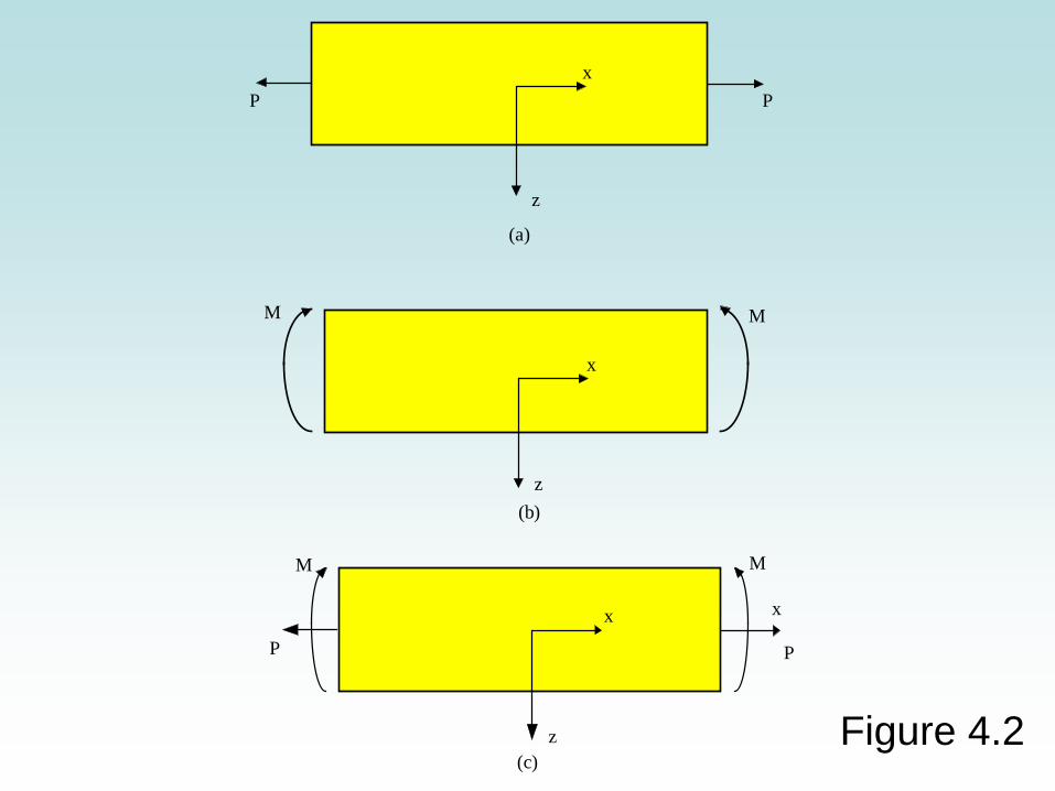
Figure 4.2

x

P

PP

P

z

x

(a)

z(c)

x

z

M M

(b)

x

MM

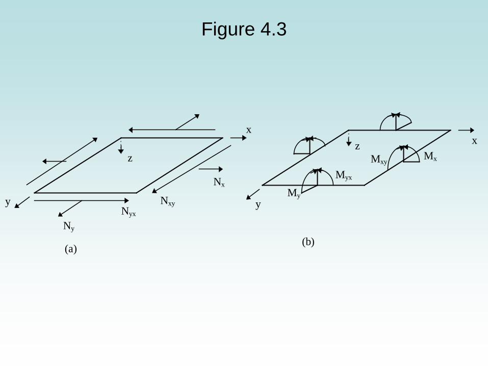
Figure 4.3

x

y

z

Ny

Nx

NxyNyx

(a)

y

xz

My

Myx

MxyMx

(b)

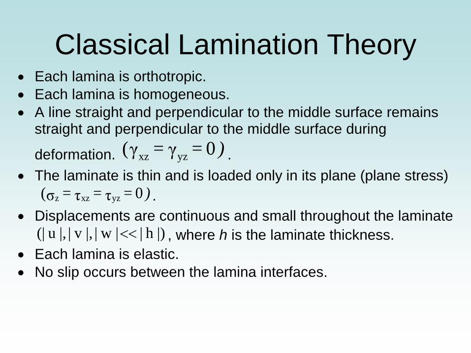
Classical Lamination Theory • Each lamina is orthotropic. • Each lamina is homogeneous. • A line straight and perpendicular to the middle surface remains

straight and perpendicular to the middle surface during

deformation. )0 = γ = γ( yzxz . • The laminate is thin and is loaded only in its plane (plane stress)

)0 = τ = τ = σ( yzxzz . • Displacements are continuous and small throughout the laminate

|)h| |w| |,v| |,u(| << , where h is the laminate thickness. • Each lamina is elastic. • No slip occurs between the lamina interfaces.

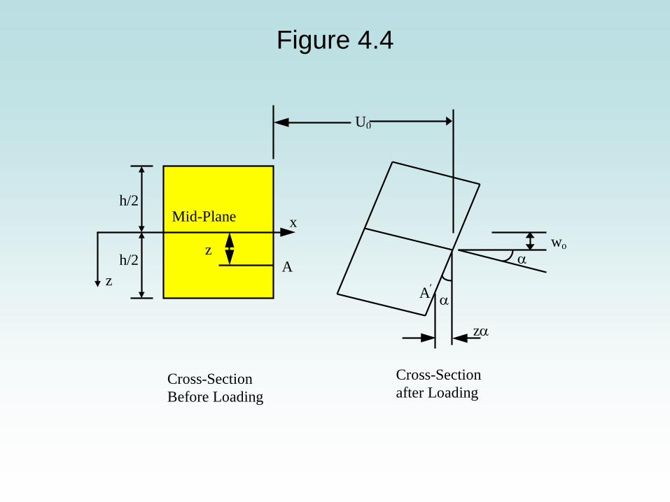
Figure 4.4

Cross-Section after Loading

x

U0

z

zα

A′

α

α

z A

Mid-Plane

wo

Cross-Section Before Loading

h/2

h/2

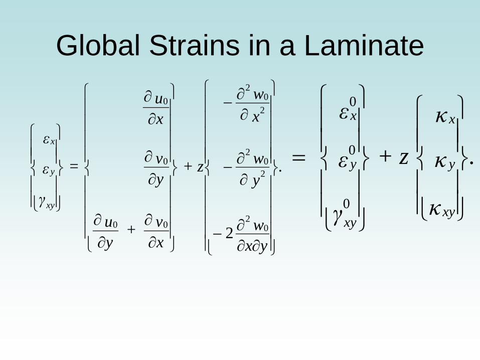
Global Strains in a Laminate

.

yxw

yw

xw

+ z

xv +

yu

yv

xu

=

γ

ε

ε

xy

y

x

∂∂∂−

∂∂−

∂∂−

∂∂

∂∂

∂∂

∂∂

02

20

2

20

2

00

0

0

2

.

κ

κ

κ

+ z

γ

ε

ε

xy

y

x

xy

y

x

=

0

0

0

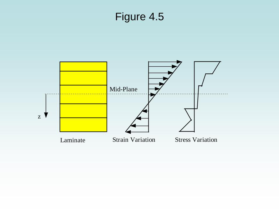
Figure 4.5

z

Mid-Plane

Strain Variation Stress VariationLaminate

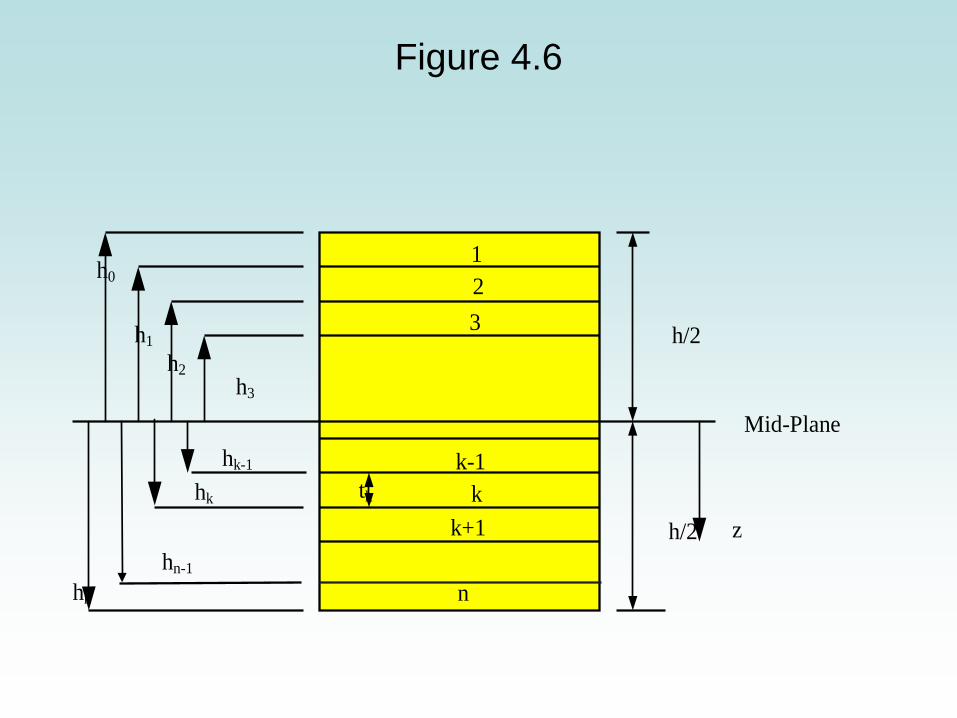
Figure 4.6

hk-1 hk

hn

h2 h1

h0

Mid-Plane

1 2 3

n

k-1 k

k+1

h3

z

h/2

tk

hn-1 h/2

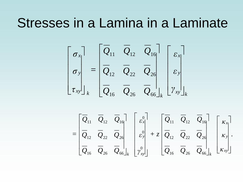
Stresses in a Lamina in a Laminate

kxy

y

x

k kxy

y

x

γ

ε

ε

QQQ

QQQ

QQQ

=

τ

σ

σ

662616

262212

161211

.

κ

κ

κ

QQQ

QQQ

QQQ

+ z

γ

ε

ε

QQQ

QQQ

QQQ

=

xy

y

x

kxy

y

x

k

662616

262212

161211

0

0

0

662616

262212

161211

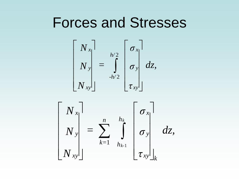
Forces and Stresses

dz,

τ

σ

σ

=

N

N

N

xy

y

xh/

-h/

xy

y

x

∫2

2

dz,

τ

σ

σ

=

N

N

N

xy

y

x

k

h

h

n

k=

xy

y

xk

k-

∫∑11

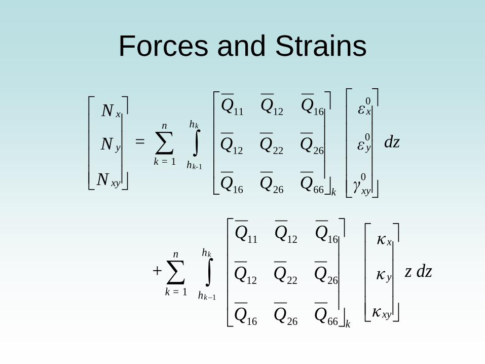
Forces and Strains

dz

γ

ε

ε

QQQ

QQQ

QQQ

=

N

N

N

xy

y

x

k

h

h

n

k =

xy

y

xk

k-

∫∑0

0

0

662616

262212

161211

1 1

z dz

κ

κ

κ

QQQ

QQQ

QQQ

+

xy

y

x

k

h

h

n

k =

k

k

∫∑−

662616

262212

161211

1 1

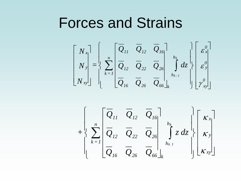
Forces and Strains

∫∑γ

ε

ε

0xy

0y

0x

h

h

662616

262212

161211

k

n

1 = k

xy

y

x

dz

QQQ

QQQ

QQQ

=

N

N

Nk

1 - k

∫∑κ

κ

κ

xy

y

xh

h

662616

262212

161211

k

n

1 = k

dz z

QQQ

QQQ

QQQ

+k

1 k

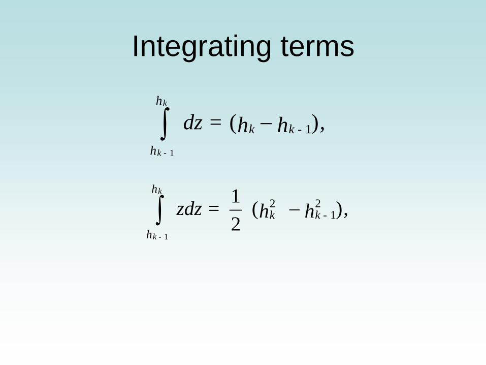
Integrating terms

,hh dz = k - k

h

h

k

k -

)( 1

1

−∫

,h h zdz = k - k

h

h

k

k -

)(21 2

12

1

−∫

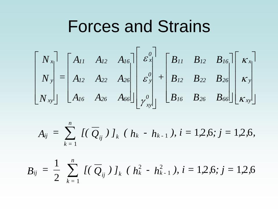
Forces and Strains

κ

κ

κ

γ

ε

ε

xy

y

x

662616

262212

161211

0xy

0y

0x

662616

262212

161211

xy

y

x

BBB

BBB

BBB

+

AAA

AAA

AAA

=

N

N

N

,,,; j = ,,), i = h - h (])Q [( = A k - kkij

n

k = ij 6216211

1∑

62162121 2

12

1

,,; j = ,,), i = h - h (])Q [( = B k - kkij

n

k = ij ∑

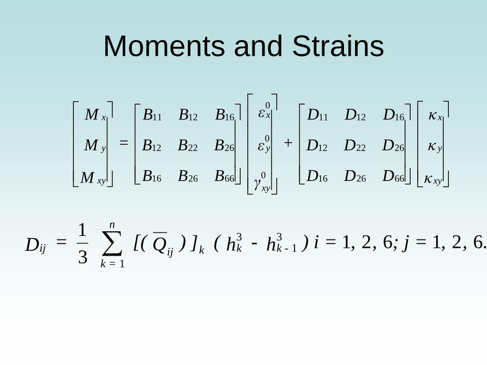
Moments and Strains

κ

κ

κ

DDD

DDD

DDD

+

γ

ε

ε

BBB

BBB

BBB

=

M

M

M

xy

y

x

xy

y

x

xy

y

x

662616

262212

161211

0

0

0

662616

262212

161211

., , ; j = , , ) i = h - h (])Q [( = D k - kkij

n

k = ij 621621

31 3

13

1∑

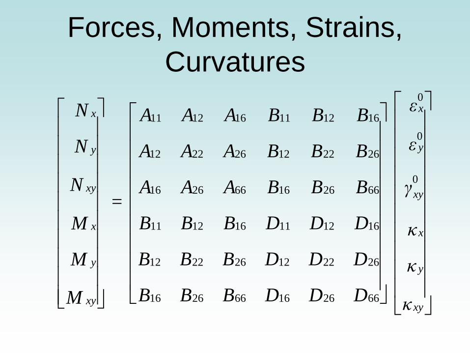
Forces, Moments, Strains, Curvatures

κ

κ

κ

γ

ε

ε

DDDBBB

DDDBBB

DDDBBB

BBBAAA

BBBAAA

BBBAAA

=

M

M

M

N

N

N

xy

y

x

xy

y

x

xy

y

x

xy

y

x

0

0

0

662616662616

262212262212

161211161211

662616662616

262212262212

161211161211

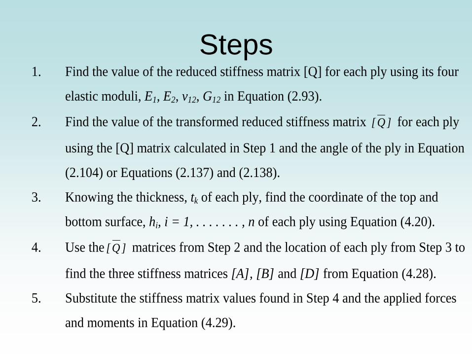
Steps 1. Find the value of the reduced stiffness matrix [Q] for each ply using its four

elastic moduli, E1, E2, v12, G12 in Equation (2.93).

2. Find the value of the transformed reduced stiffness matrix ]Q[ for each ply

using the [Q] matrix calculated in Step 1 and the angle of the ply in Equation

(2.104) or Equations (2.137) and (2.138).

3. Knowing the thickness, tk of each ply, find the coordinate of the top and

bottom surface, hi, i = 1, . . . . . . . , n of each ply using Equation (4.20).

4. Use the ]Q[ matrices from Step 2 and the location of each ply from Step 3 to

find the three stiffness matrices [A], [B] and [D] from Equation (4.28).

5. Substitute the stiffness matrix values found in Step 4 and the applied forces

and moments in Equation (4.29).

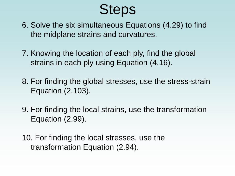
Steps 6. Solve the six simultaneous Equations (4.29) to find

the midplane strains and curvatures. 7. Knowing the location of each ply, find the global

strains in each ply using Equation (4.16). 8. For finding the global stresses, use the stress-strain

Equation (2.103). 9. For finding the local strains, use the transformation

Equation (2.99). 10. For finding the local stresses, use the

transformation Equation (2.94).

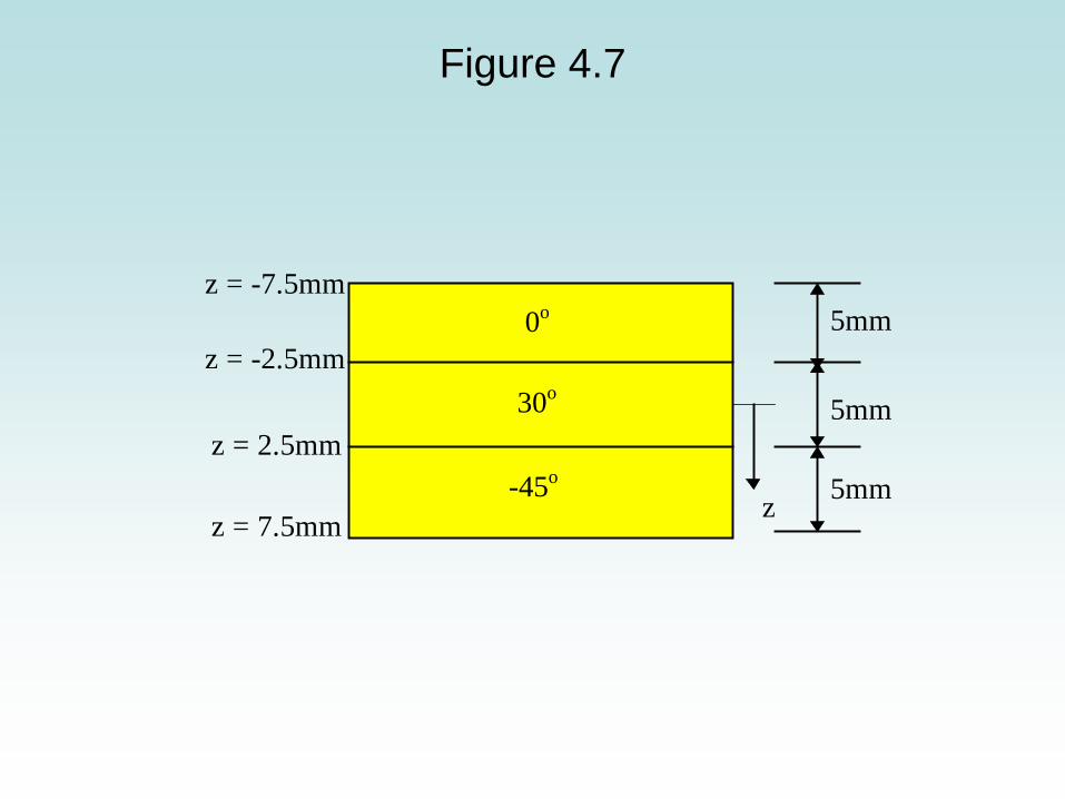
Figure 4.7

0o

30o

-45o

5mm

5mm

5mm

z = -2.5mm

z = 2.5mm

z = 7.5mm z

z = -7.5mm

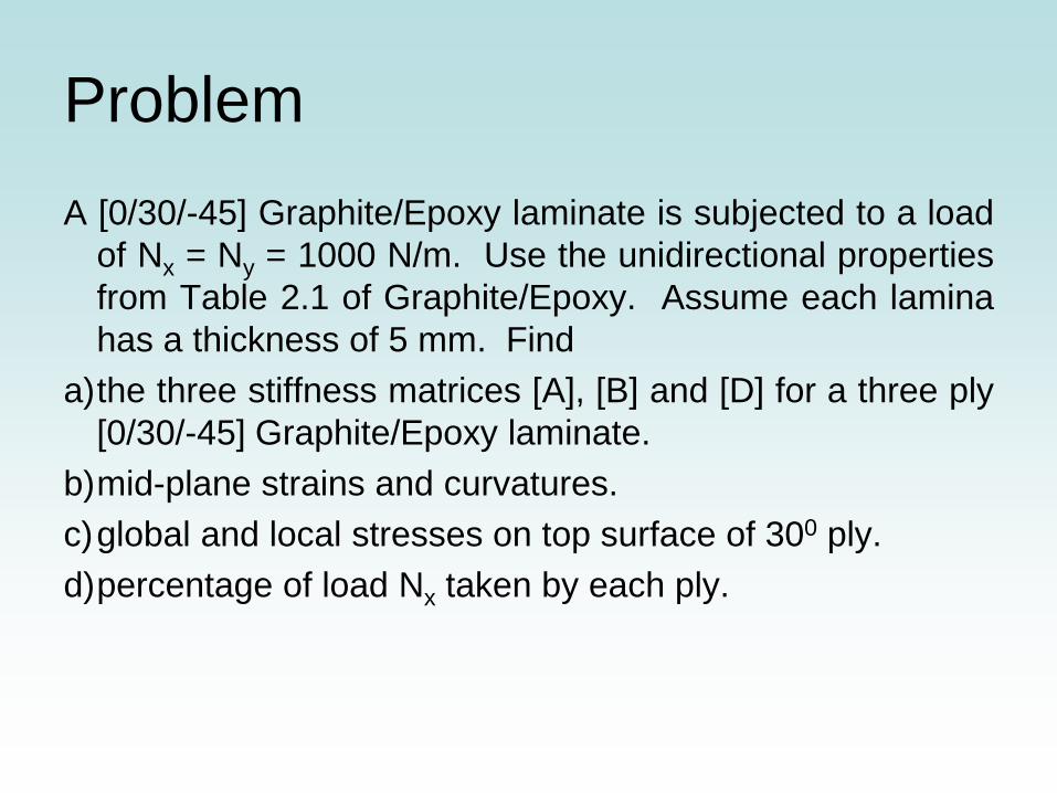
Problem A [0/30/-45] Graphite/Epoxy laminate is subjected to a load

of Nx = Ny = 1000 N/m. Use the unidirectional properties from Table 2.1 of Graphite/Epoxy. Assume each lamina has a thickness of 5 mm. Find

a)the three stiffness matrices [A], [B] and [D] for a three ply [0/30/-45] Graphite/Epoxy laminate.

b)mid-plane strains and curvatures. c)global and local stresses on top surface of 300 ply. d)percentage of load Nx taken by each ply.

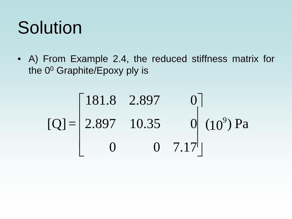
Solution • A) From Example 2.4, the reduced stiffness matrix for

the 00 Graphite/Epoxy ply is

0

Pa)10(

7.1700

010.352.897

02.897181.8

= [Q] 9

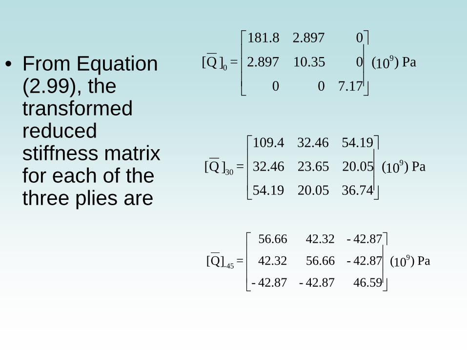
• From Equation

(2.99), the transformed reduced stiffness matrix for each of the three plies are

Pa)10(

7.1700

010.352.897

02.897181.8

= ]Q[ 90

Pa)10(

36.7420.0554.19

20.0523.6532.46

54.1932.46109.4

= ]Q[ 930

Pa)10(

46.5942.87-42.87-

42.87-56.6642.32

42.87-42.3256.66

= ]Q[ 945-

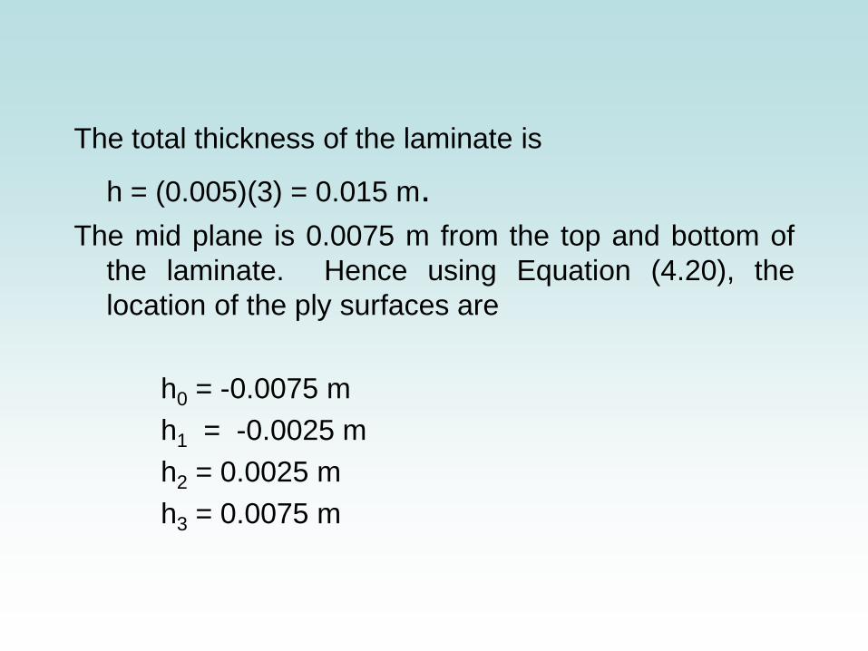
The total thickness of the laminate is

h = (0.005)(3) = 0.015 m. The mid plane is 0.0075 m from the top and bottom of

the laminate. Hence using Equation (4.20), the location of the ply surfaces are

h0 = -0.0075 m h1 = -0.0025 m h2 = 0.0025 m h3 = 0.0075 m

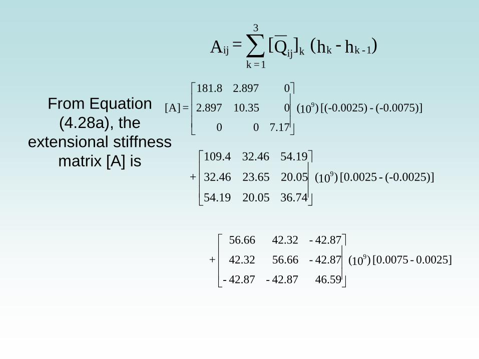
From Equation (4.28a), the

extensional stiffness matrix [A] is

(-0.0075)]-[(-0.0025) )10(

7.1700

010.352.897

02.897181.8

= [A] 9

(-0.0025)]-[0.0025 )10(

36.7420.0554.19

20.0523.6532.46

54.1932.46109.4

+ 9

0.0025]-[0.0075 )10(

46.5942.87-42.87-

42.87-56.6642.32

42.87-42.3256.66

+ 9

)h - h( ]Q[ = A 1 -k kkij

3

1 =k ij ∑

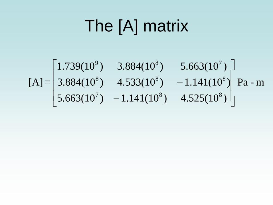
The [A] matrix

m- Pa)4.525(10)1.141(10)5.663(10)1.141(10)4.533(10)3.884(10

)5.663(10)3.884(10)1.739(10 = [A]

887

888

789

−−

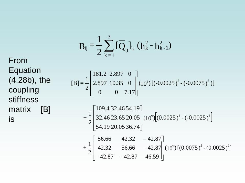
From Equation (4.28b), the coupling stiffness matrix [B] is

)h - h( ]Q[

21 = B 2

1 -k 2kkij

3

1 =k ij ∑

)] )(-0.0075 - )[(-0.0025 )10( 7.17

00

010.352.897

0

2.897181.2

21 = [B] 229

[ ])(-0.0025 - )(0.0025)10( 36.7420.0554.19

20.0523.6532.46

54.1932.46109.4

21 + 229

])(0.0025 - )[(0.0075 )10( 46.5942.8742.8742.8756.6642.3242.8742.3256.66

21 + 229

−−−−

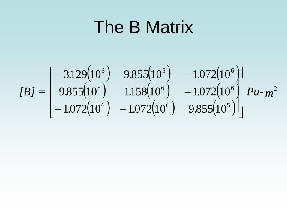
The B Matrix

( ) ( ) ( )( ) ( ) ( )( ) ( ) ( )

m Pa-.........

[B] = 2

566

665

656

108559100721100721100721101581108559100721108559101293

−−−−−

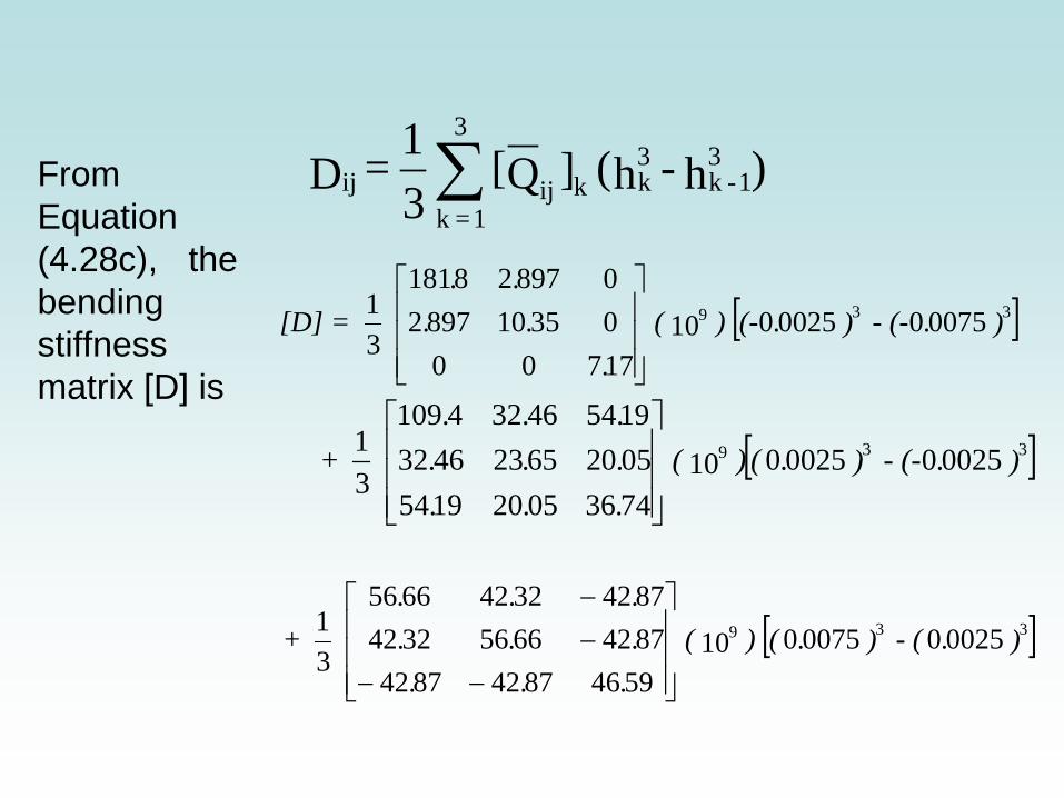
From Equation (4.28c), the bending stiffness matrix [D] is

)h - h( ]Q[

31 = D 3

1 -k 3kkij

3

1 =k ij ∑

[ ]). - (-).(-) (.

....

[D] = 339 00750002501017700035108972089728181

31

[ ]). - (-).() (.........

+ 339 002500025010743605201954052065234632195446324109

31

[ ]). - ().() (.........

+ 339 002500075010594687428742874266563242874232426656

31

−−−−

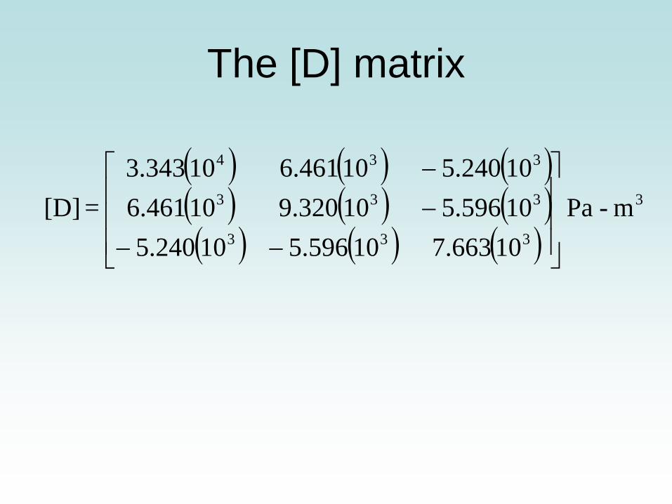
The [D] matrix

( ) ( ) ( )( ) ( ) ( )( ) ( ) ( )

3

333

333

334

m- Pa107.663105.596105.240105.596109.320106.461105.240106.461103.343

= [D]

−−−−

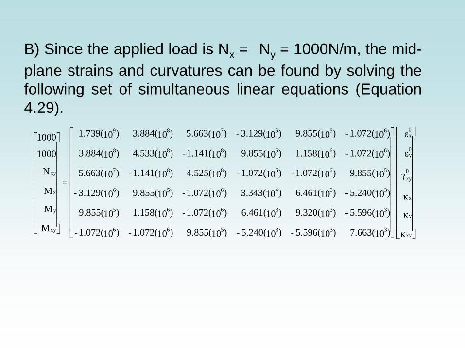
B) Since the applied load is Nx = Ny = 1000N/m, the mid-plane strains and curvatures can be found by solving the following set of simultaneous linear equations (Equation 4.29).

κ

κ

κ

γ

ε

ε

)107.663()105.596(-)105.240(-)109.855()101.072(-)101.072(-

)105.596(-)109.320()106.461()101.072(-)101.158()109.855(

)105.240(-)106.461()103.343()101.072(-)109.855()103.129(-

)109.855()101.072(-)101.072(-)104.525()101.141(-)105.663(

)101.072(-)101.158()109.855()101.141(-)104.533()103.884(

)101.072(-)109.855()103.129(-)105.663()103.884()101.739(

=

M

M

M

N

1000

1000

xy

y

x

0xy

0y

0x

333566

333665

334656

566887

665888

656789

xy

y

x

xy

1/m

)104.101(

)103.285(-

)102.971(

m/m

)107.598(-

)103.492(

)103.123(

=

κ

κ

κ

γ

ε

ε

4-

4-

5-

7-

6-

7-

xy

y

x

0xy

0y

0x

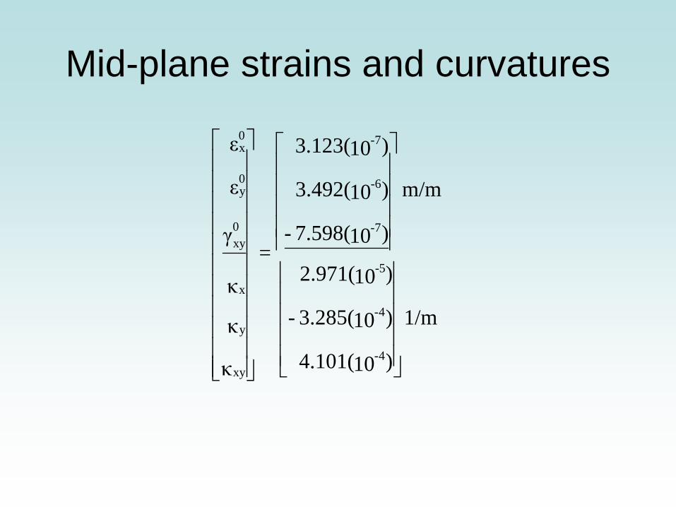
Mid-plane strains and curvatures

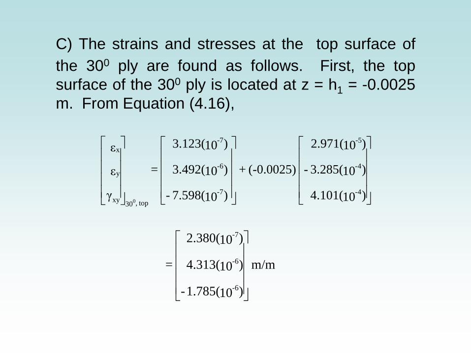
C) The strains and stresses at the top surface of the 300 ply are found as follows. First, the top surface of the 300 ply is located at z = h1 = -0.0025 m. From Equation (4.16),

)104.101(

)103.285(-

)102.971(

(-0.0025) +

)107.598(-

)103.492(

)103.123(

=

γ

ε

ε

4-

4-

-5

7-

6-

-7

xy

y

x

top,300

m/m

)101.785(-

)104.313(

)102.380(

=

6-

6-

-7

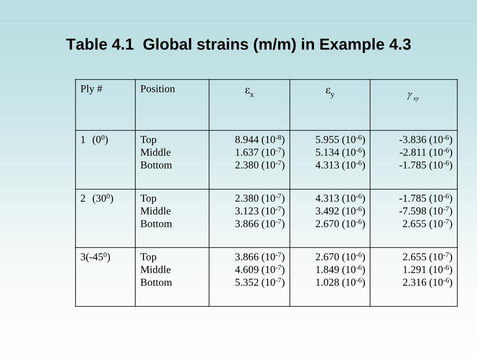
Table 4.1 Global strains (m/m) in Example 4.3

γ xyPly # Position εx εy

1 (00) Top Middle Bottom

8.944 (10-8) 1.637 (10-7) 2.380 (10-7)

5.955 (10-6) 5.134 (10-6) 4.313 (10-6)

-3.836 (10-6) -2.811 (10-6) -1.785 (10-6)

2 (300) Top Middle Bottom

2.380 (10-7) 3.123 (10-7) 3.866 (10-7)

4.313 (10-6) 3.492 (10-6) 2.670 (10-6)

-1.785 (10-6) -7.598 (10-7) 2.655 (10-7)

3(-450) Top Middle Bottom

3.866 (10-7) 4.609 (10-7) 5.352 (10-7)

2.670 (10-6) 1.849 (10-6) 1.028 (10-6)

2.655 (10-7) 1.291 (10-6) 2.316 (10-6)

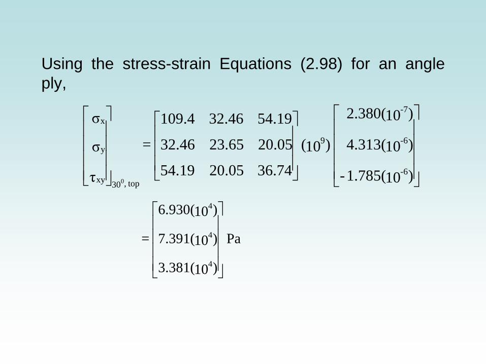
Using the stress-strain Equations (2.98) for an angle ply,

)101.785(-

)104.313(

)102.380(

)10(

36.7420.0554.19

20.0523.6532.46

54.1932.46109.4

=

τ

σ

σ

6-

6-

-7

9

xy

y

x

top,300

Pa

)103.381(

)107.391(

)106.930(

=

4

4

4

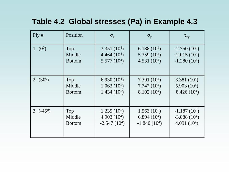
Table 4.2 Global stresses (Pa) in Example 4.3

Ply # Position σx σy τxy

1 (00) Top Middle Bottom

3.351 (104) 4.464 (104) 5.577 (104)

6.188 (104) 5.359 (104) 4.531 (104)

-2.750 (104) -2.015 (104) -1.280 (104)

2 (300) Top Middle Bottom

6.930 (104) 1.063 (105) 1.434 (105)

7.391 (104) 7.747 (104) 8.102 (104)

3.381 (104) 5.903 (104) 8.426 (104)

3 (-450) Top Middle Bottom

1.235 (105) 4.903 (104) -2.547 (104)

1.563 (105) 6.894 (104) -1.840 (104)

-1.187 (105) -3.888 (104) 4.091 (104)

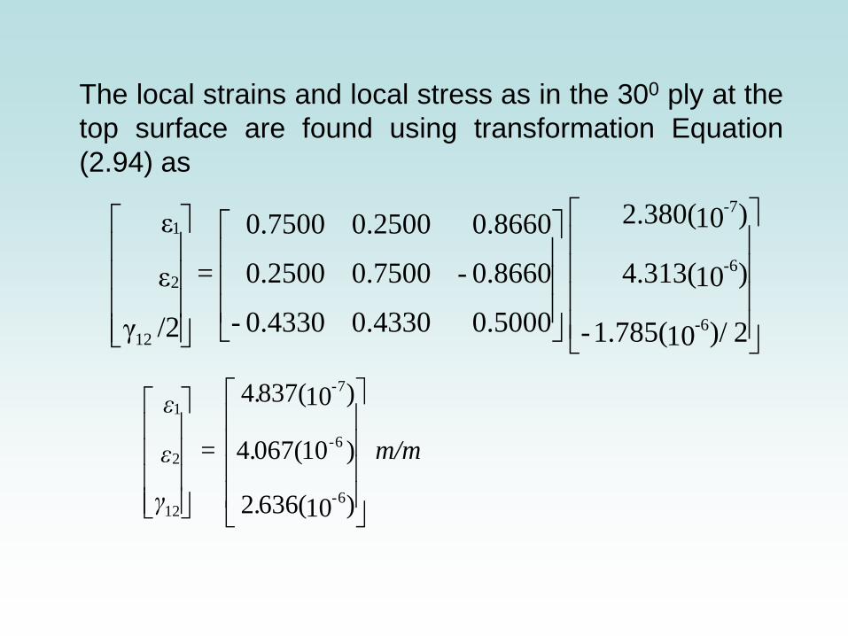
The local strains and local stress as in the 300 ply at the top surface are found using transformation Equation (2.94) as

2)/ 101.785(-

)104.313(

)102.380(

0.50000.43300.4330-

0.8660-0.75000.2500

0.86600.25000.7500

=

/2γ

ε

ε

6-

6-

-7

12

2

1

m/m

.

.

.

=

γ

ε

ε

-

-

-

)10(6362

)10(0674

)10(8374

6

6

7

12

2

1

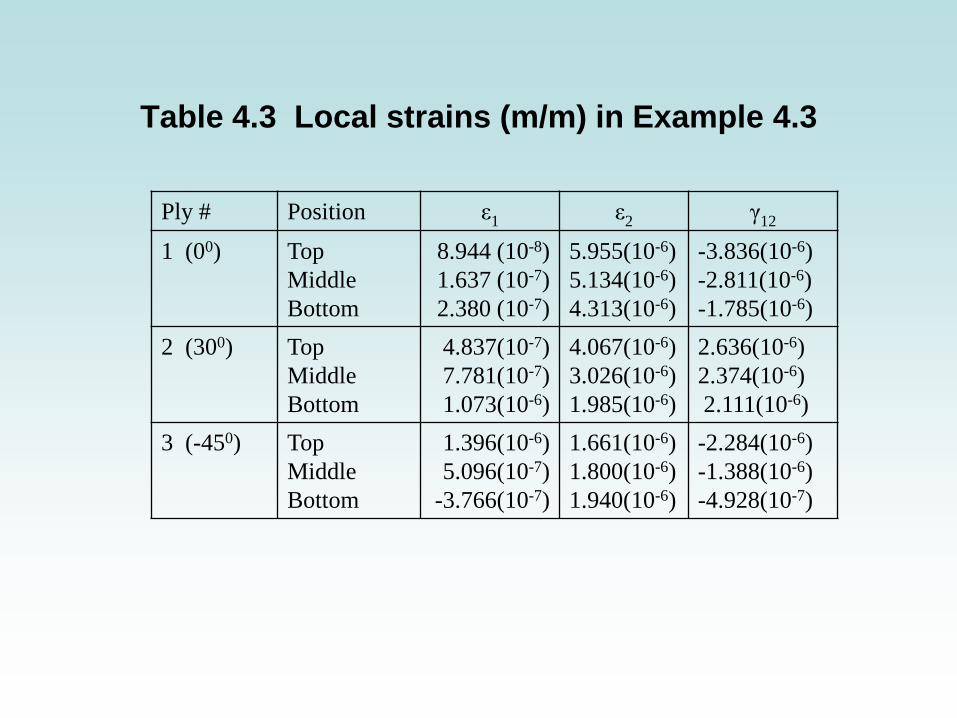
Table 4.3 Local strains (m/m) in Example 4.3

Ply # Position ε1 ε2 γ12

1 (00) Top Middle Bottom

8.944 (10-8) 1.637 (10-7) 2.380 (10-7)

5.955(10-6) 5.134(10-6) 4.313(10-6)

-3.836(10-6) -2.811(10-6) -1.785(10-6)

2 (300) Top Middle Bottom

4.837(10-7) 7.781(10-7) 1.073(10-6)

4.067(10-6) 3.026(10-6) 1.985(10-6)

2.636(10-6) 2.374(10-6) 2.111(10-6)

3 (-450) Top Middle Bottom

1.396(10-6) 5.096(10-7)

-3.766(10-7)

1.661(10-6) 1.800(10-6) 1.940(10-6)

-2.284(10-6) -1.388(10-6) -4.928(10-7)

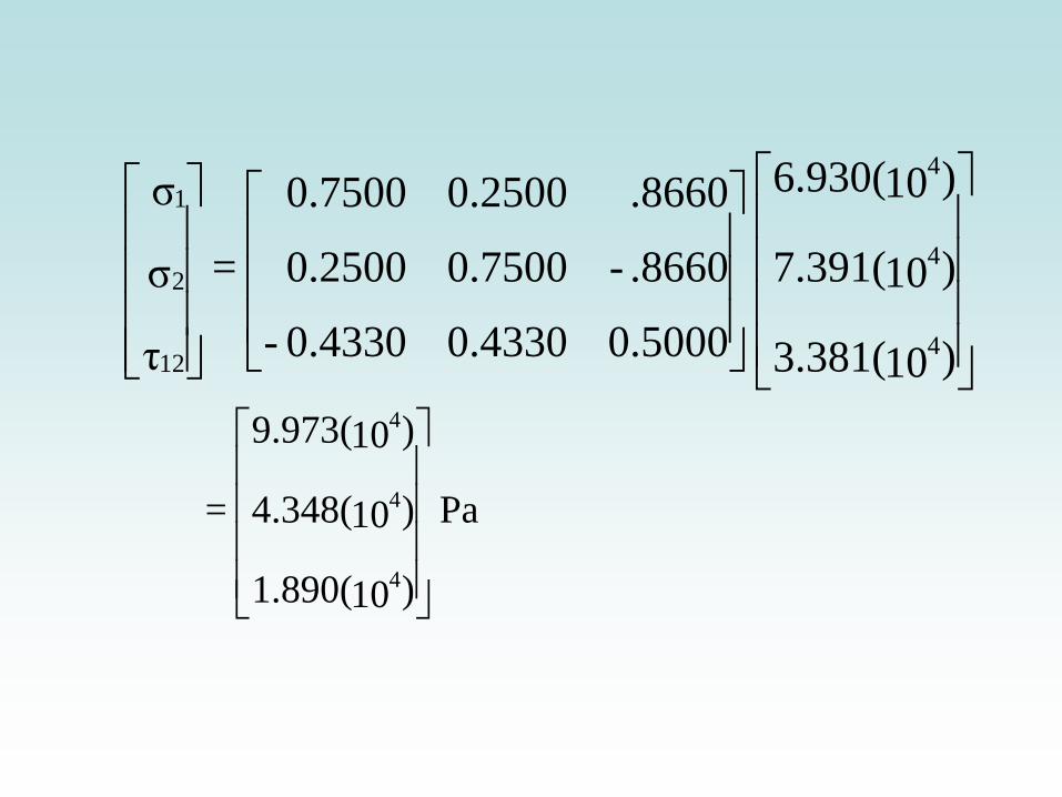
)103.381(

)107.391(

)106.930(

0.50000.43300.4330-

.8660-0.75000.2500

.86600.25000.7500

=

τ

σ

σ

4

4

4

12

2

1

Pa

)101.890(

)104.348(

)109.973(

=

4

4

4

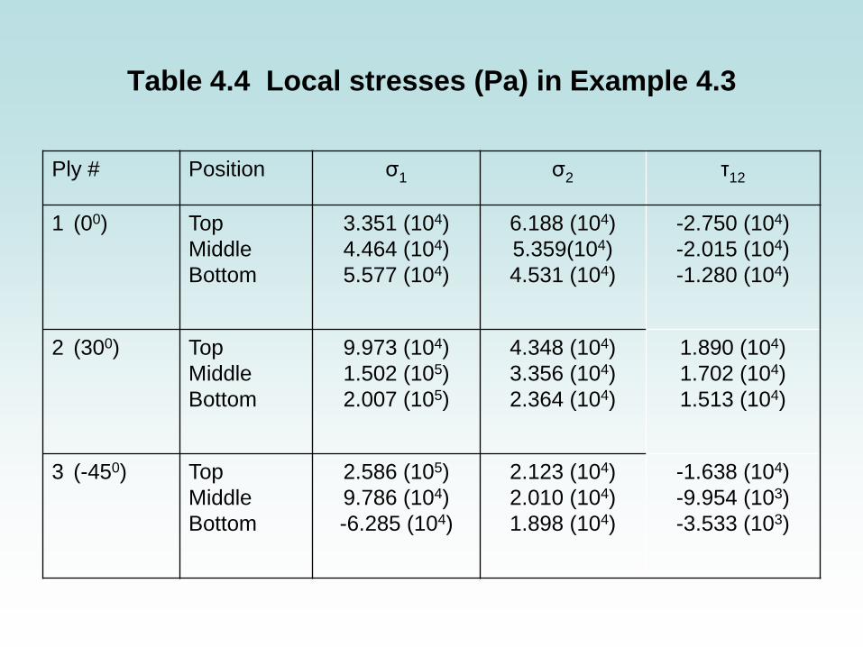
Table 4.4 Local stresses (Pa) in Example 4.3

Ply # Position σ1 σ2 τ12

1 (00) Top Middle Bottom

3.351 (104) 4.464 (104) 5.577 (104)

6.188 (104) 5.359(104) 4.531 (104)

-2.750 (104) -2.015 (104) -1.280 (104)

2 (300) Top Middle Bottom

9.973 (104) 1.502 (105) 2.007 (105)

4.348 (104) 3.356 (104) 2.364 (104)

1.890 (104) 1.702 (104) 1.513 (104)

3 (-450) Top Middle Bottom

2.586 (105) 9.786 (104) -6.285 (104)

2.123 (104) 2.010 (104) 1.898 (104)

-1.638 (104) -9.954 (103) -3.533 (103)

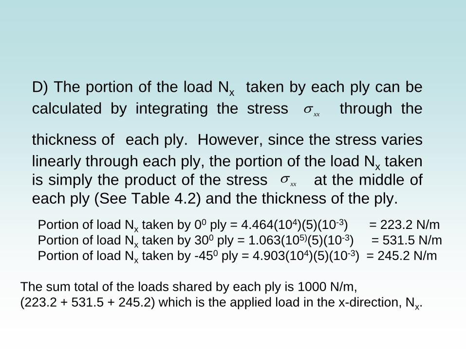
D) The portion of the load Nx taken by each ply can be calculated by integrating the stress through the

thickness of each ply. However, since the stress varies linearly through each ply, the portion of the load Nx taken is simply the product of the stress at the middle of each ply (See Table 4.2) and the thickness of the ply.

Portion of load Nx taken by 00 ply = 4.464(104)(5)(10-3) = 223.2 N/m Portion of load Nx taken by 300 ply = 1.063(105)(5)(10-3) = 531.5 N/m Portion of load Nx taken by -450 ply = 4.903(104)(5)(10-3) = 245.2 N/m The sum total of the loads shared by each ply is 1000 N/m, (223.2 + 531.5 + 245.2) which is the applied load in the x-direction, Nx.

σ xx

σ xx

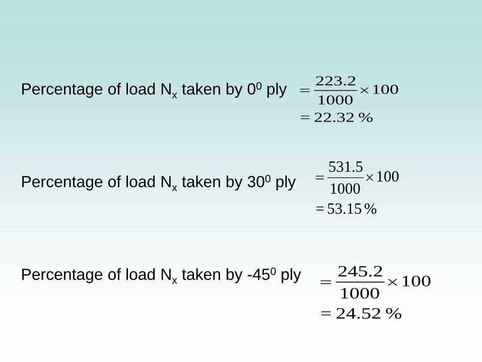
Percentage of load Nx taken by 00 ply Percentage of load Nx taken by 300 ply Percentage of load Nx taken by -450 ply

% 22.32 =

1001000223.2 ×=

% 53.15 =

100 1000531.5 ×=

% 24.52 =

100 1000245.2 ×=

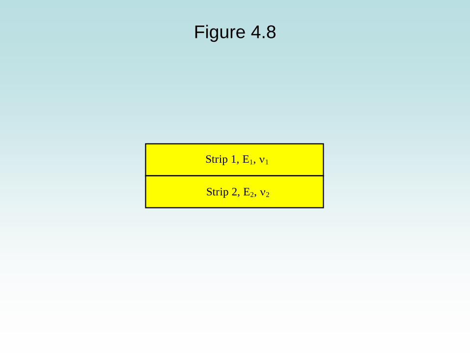
Figure 4.8

Strip 1, E1, ν1

Strip 2, E2, ν2