
Macroeconomics for Development -
19
MSc in Economics for Development Macroeconomics for Development Week 4 Class Sam Wills Department of Economics, University of Oxford [email protected] Consultation hours: Friday, 2-3pm, Weeks 1,3-8 (MT) 01 November 2011 Macro for Development Class 4 1
Transcript of Macroeconomics for Development -

MSc in Economics for Development
Macroeconomics for Development Week 4 Class
Sam Wills
Department of Economics, University of Oxford
Consultation hours: Friday, 2-3pm, Weeks 1,3-8 (MT)
01 November 2011
Macro for Development Class 4 1
Week 3 Review
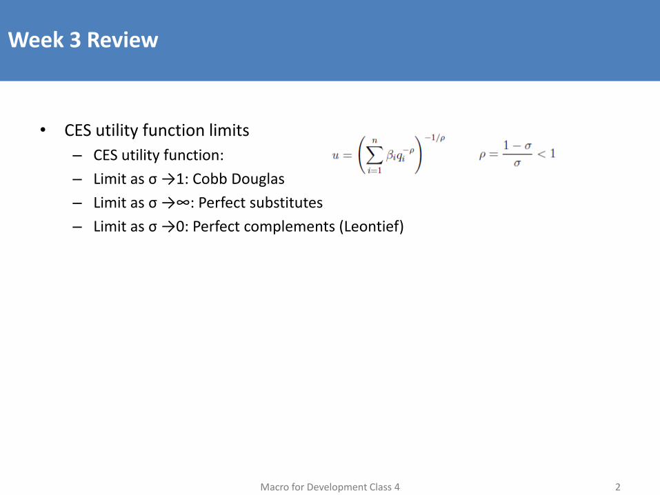
• CES utility function limits
– CES utility function:
– Limit as σ →1: Cobb Douglas
– Limit as σ →∞: Perfect substitutes
– Limit as σ →0: Perfect complements (Leontief)
Macro for Development Class 4 2
Week 4 References
• Heijdra, B. J., Van der Ploeg, F., 2002, Foundations of Modern Macroeconomics, OUP, Ch 11.1
– Brief late undergrad/graduate level look at IS-LM model
• Dornbusch, R., Fischer, S., Startz, R., 2008, Macroeconomics, McGraw Hill, Ch 12 and 20
– Early undergrad look at IS-LM with plenty of diagrams and intuitive link to national accounts
• Also try any other undergrad text
Macro for Development Class 4 3
Overview: The Mundell-Fleming Model
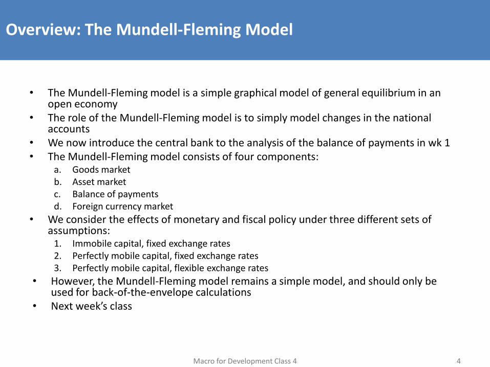
• The Mundell-Fleming model is a simple graphical model of general equilibrium in an open economy
• The role of the Mundell-Fleming model is to simply model changes in the national accounts
• We now introduce the central bank to the analysis of the balance of payments in wk 1 • The Mundell-Fleming model consists of four components:
a. Goods market b. Asset market c. Balance of payments d. Foreign currency market
• We consider the effects of monetary and fiscal policy under three different sets of assumptions:
1. Immobile capital, fixed exchange rates 2. Perfectly mobile capital, fixed exchange rates 3. Perfectly mobile capital, flexible exchange rates
• However, the Mundell-Fleming model remains a simple model, and should only be used for back-of-the-envelope calculations
• Next week’s class
Macro for Development Class 4 4
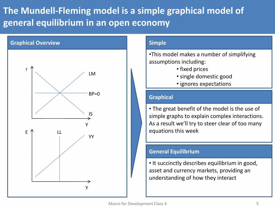
The Mundell-Fleming model is a simple graphical model of general equilibrium in an open economy
Macro for Development Class 4 5
Graphical Overview
Y
r LM
IS
BP=0
Y
E YY
LL
•This model makes a number of simplifying assumptions including:
• fixed prices • single domestic good • ignores expectations
Simple
• The great benefit of the model is the use of simple graphs to explain complex interactions. As a result we’ll try to steer clear of too many equations this week
Graphical
• It succinctly describes equilibrium in good, asset and currency markets, providing an understanding of how they interact
General Equilibrium
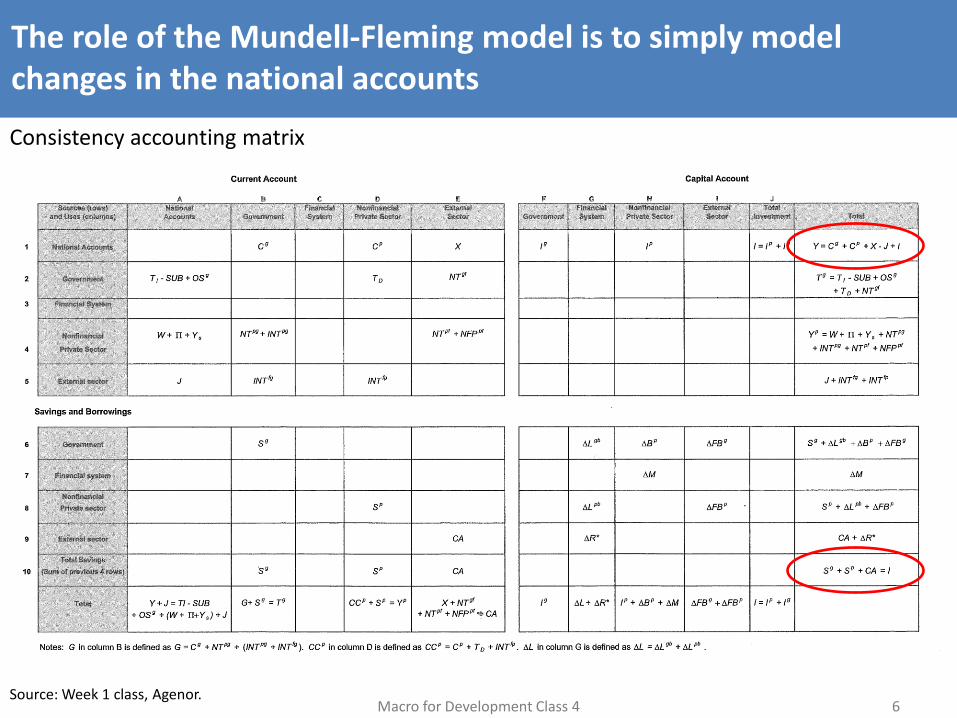
The role of the Mundell-Fleming model is to simply model changes in the national accounts
Macro for Development Class 4 6
Consistency accounting matrix
Source: Week 1 class, Agenor.
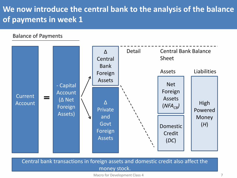
We now introduce the central bank to the analysis of the balance of payments in week 1
Macro for Development Class 4 7
Current Account
- Capital Account (Δ Net
ForeignAssets)
Δ Private
and Govt
Foreign Assets
Δ Central
Bank ForeignAssets
Domestic Credit (DC)
High Powered Money
(H)
Net Foreign Assets (NFACB)
Detail Central Bank Balance Sheet
Liabilities Assets
Balance of Payments
Central bank transactions in foreign assets and domestic credit also affect the money stock.

The Mundell-Fleming model consists of four components
Macro for Development Class 4 8
a.Goods Market
IS Curve: Y = A(r,Y) + G + NX(Y,E) A(r,Y) = C(Y) + I(r,Y)
b.Asset Market
LM Curve: M/P = L(r,Y)
c.Balance of Payments
BP Curve BP = NX(Y,E) + KA(r-r*)
Graphical Overview of the Mundell-Fleming Model
d. Foreign Currency Market
Fixed: E=E* LL: M = L(r,Y) YY: Y = A(r,Y) + G + NX(Y,E)
Y
r LM
IS
BP=0
Y
E YY
LL
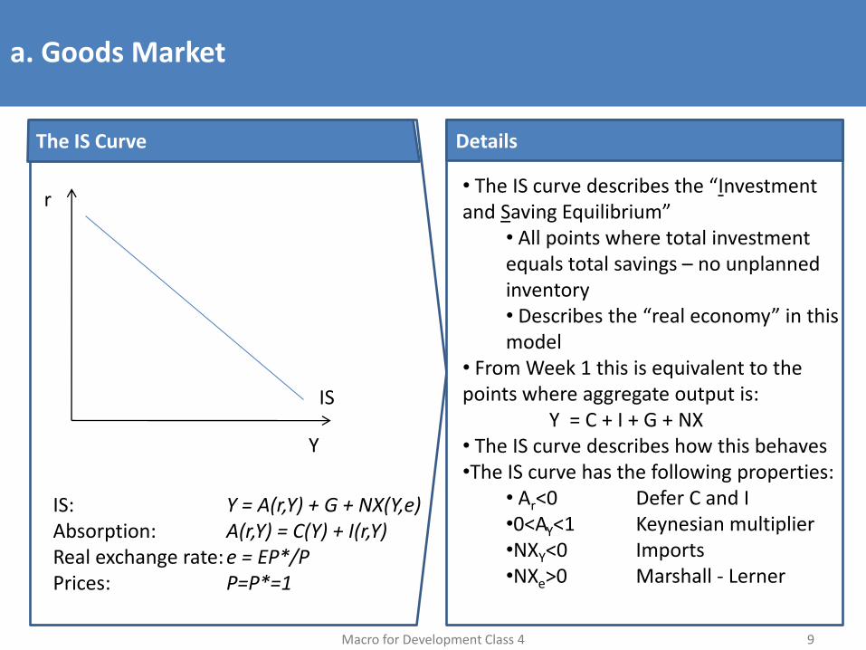
a. Goods Market
Macro for Development Class 4 9
The IS Curve
Y
r
IS
IS: Y = A(r,Y) + G + NX(Y,e) Absorption: A(r,Y) = C(Y) + I(r,Y) Real exchange rate: e = EP*/P Prices: P=P*=1
Details
• The IS curve describes the “Investment and Saving Equilibrium”
• All points where total investment equals total savings – no unplanned inventory • Describes the “real economy” in this model
• From Week 1 this is equivalent to the points where aggregate output is:
Y = C + I + G + NX • The IS curve describes how this behaves •The IS curve has the following properties:
• Ar<0 Defer C and I •0<AY<1 Keynesian multiplier •NXY<0 Imports •NXe>0 Marshall - Lerner
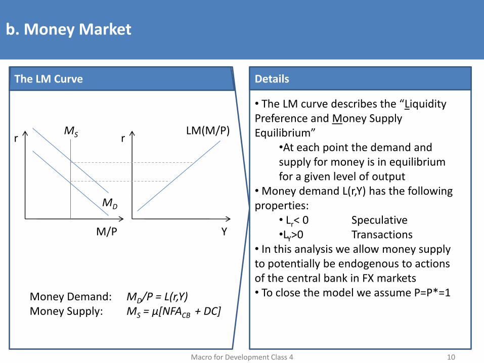
b. Money Market
Macro for Development Class 4 10
The LM Curve
Y
r LM(M/P)
Money Demand: MD/P = L(r,Y) Money Supply: MS = μ[NFACB + DC]
Details
• The LM curve describes the “Liquidity Preference and Money Supply Equilibrium”
•At each point the demand and supply for money is in equilibrium for a given level of output
• Money demand L(r,Y) has the following properties:
• Lr< 0 Speculative •LY>0 Transactions
• In this analysis we allow money supply to potentially be endogenous to actions of the central bank in FX markets • To close the model we assume P=P*=1
M/P
r MS
MD
c. Balance of Payments
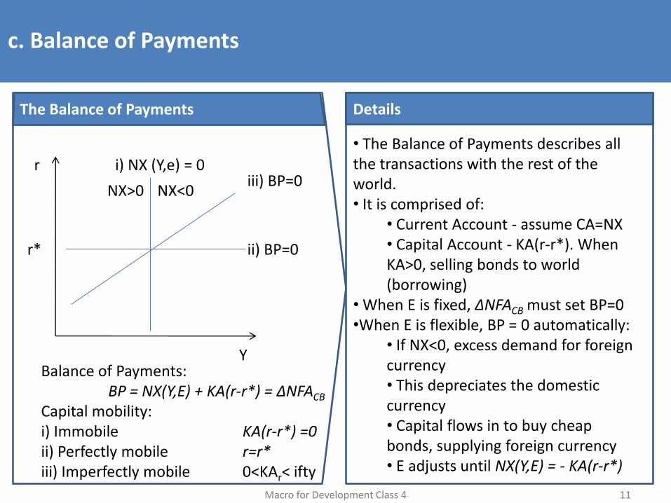
Macro for Development Class 4 11
The Balance of Payments
Balance of Payments: BP = NX(Y,E) + KA(r-r*) = ΔNFACB
Capital mobility: i) Immobile KA(r-r*) =0 ii) Perfectly mobile r=r* iii) Imperfectly mobile 0<KAr< ifty
Details
• The Balance of Payments describes all the transactions with the rest of the world. • It is comprised of:
• Current Account - assume CA=NX • Capital Account - KA(r-r*). When KA>0, selling bonds to world (borrowing)
• When E is fixed, ΔNFACB must set BP=0 •When E is flexible, BP = 0 automatically:
• If NX<0, excess demand for foreign currency • This depreciates the domestic currency • Capital flows in to buy cheap bonds, supplying foreign currency • E adjusts until NX(Y,E) = - KA(r-r*)
Y
r iii) BP=0
i) NX (Y,e) = 0
ii) BP=0
NX<0 NX>0
r*
d. Foreign Currency Market
Macro for Development Class 4 12
The Mundell-Fleming Model Details
Fixed exchange rates • We ignore the second diagram as E=E* • The central bank must adjust the money supply, shifting LM, to ensure BP=0.
Floating exchange rates • We introduce the second diagram as output and exchange rates are linked via NX(Y,E). • We only do this with mobile capital:
• With immobile capital E adjusts so NX=0 • With mobile capital, changes in E automatically ensure that BP=0:
BP = NX(Y,E) + KA(r-r*) = ΔNFACB = 0 • The model is now a system of 3 equations in 3 variables: r, Y, E. These can be plotted as simultaneous equilibria. In (E,Y) space, high E stimulates X and thus Y.
LL: M = L(r,Y) YY: Y = A(r,Y) + G + NX(Y,E) r: r=r*
Y
r LM
IS
BP=0
Y
E YY
LL
E=E* E*
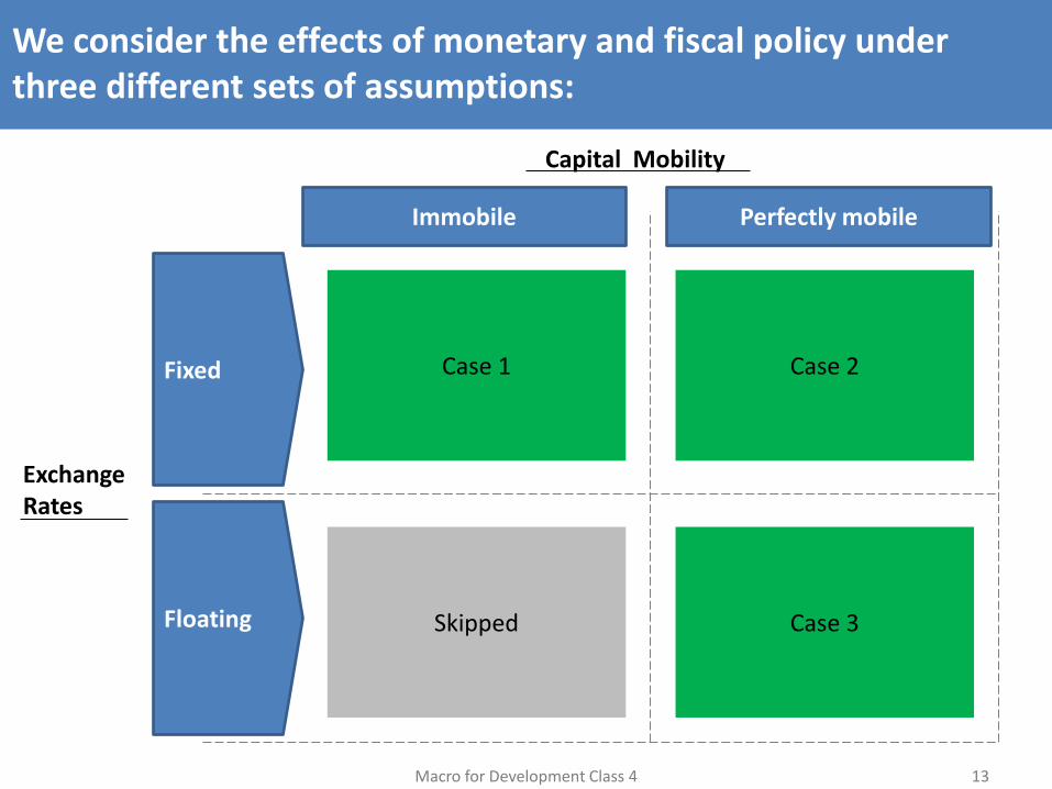
We consider the effects of monetary and fiscal policy under three different sets of assumptions:
Macro for Development Class 4 13
Capital Mobility
Exchange Rates
Case 1 Fixed
Floating
Immobile Perfectly mobile
Case 2
Skipped Case 3
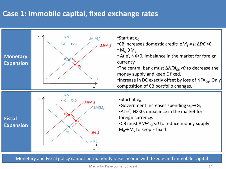
Case 1: Immobile capital, fixed exchange rates
Macro for Development Class 4 14
Monetary Expansion
•Start at e0
•CB increases domestic credit: ΔMS = μ ΔDC >0 • M0→M1 • At e’, NX<0, imbalance in the market for foreign currency. •The central bank must ΔNFACB <0 to decrease the money supply and keep E fixed. •Increase in DC exactly offset by loss of NFACB. Only composition of CB portfolio changes.
•Start at e0
•Government increases spending G0→G1
•At e”, NX<0, imbalance in the market for foreign currency. •CB must ΔNFACB <0 to reduce money supply M0→M2 to keep E fixed
Monetary and Fiscal policy cannot permanently raise income with fixed e and immobile capital
Fiscal Expansion
Y
r LM(M0)
IS
BP=0
X<0 X>0
e0
e1
LM(M1)
Y
r
LM(M0)
IS(G0)
BP=0
X<0 X>0
e0
e1
LM(M2)
IS(G1)
e”
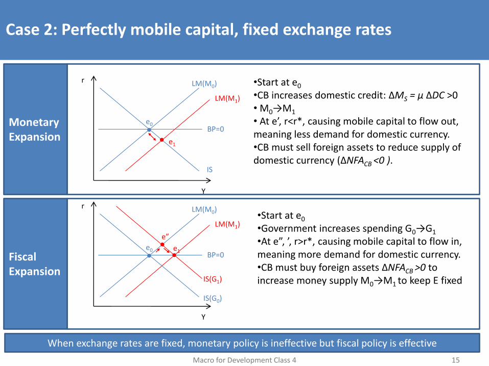
Case 2: Perfectly mobile capital, fixed exchange rates
Macro for Development Class 4 15
Monetary Expansion
•Start at e0
•CB increases domestic credit: ΔMS = μ ΔDC >0 • M0→M1 • At e’, r<r*, causing mobile capital to flow out, meaning less demand for domestic currency. •CB must sell foreign assets to reduce supply of domestic currency (ΔNFACB <0 ).
•Start at e0
•Government increases spending G0→G1
•At e”, ’, r>r*, causing mobile capital to flow in, meaning more demand for domestic currency. •CB must buy foreign assets ΔNFACB >0 to increase money supply M0→M1 to keep E fixed
When exchange rates are fixed, monetary policy is ineffective but fiscal policy is effective
Fiscal Expansion
Y
r LM(M0)
IS
BP=0 e0
e1
LM(M1)
Y
r LM(M0)
IS(G0)
BP=0 e0
e”
LM(M1)
IS(G1)
e1
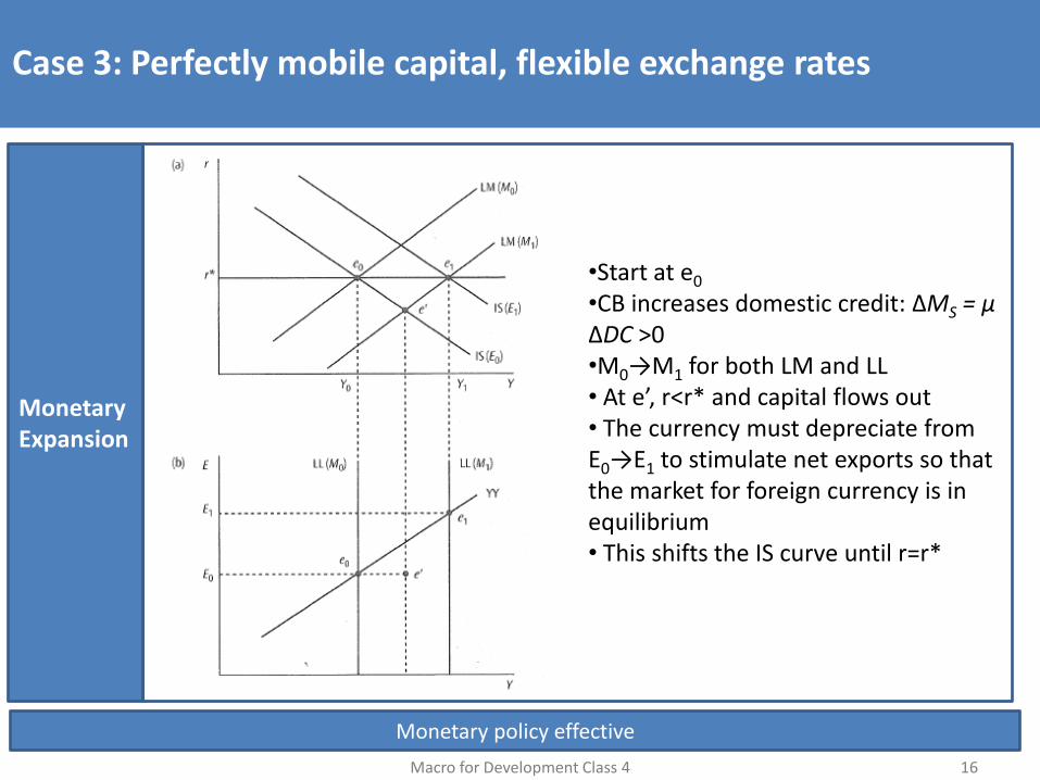
Case 3: Perfectly mobile capital, flexible exchange rates
Macro for Development Class 4 16
•Start at e0
•CB increases domestic credit: ΔMS = μ ΔDC >0 •M0→M1 for both LM and LL • At e’, r<r* and capital flows out • The currency must depreciate from E0→E1 to stimulate net exports so that the market for foreign currency is in equilibrium • This shifts the IS curve until r=r*
MonetaryExpansion
Monetary policy effective
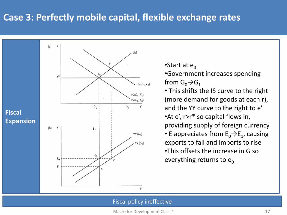
Case 3: Perfectly mobile capital, flexible exchange rates
Macro for Development Class 4 17
•Start at e0
•Government increases spending from G0→G1 • This shifts the IS curve to the right (more demand for goods at each r), and the YY curve to the right to e’ •At e’, r>r* so capital flows in, providing supply of foreign currency • E appreciates from E0→E1, causing exports to fall and imports to rise •This offsets the increase in G so everything returns to e0
Fiscal Expansion
Fiscal policy ineffective
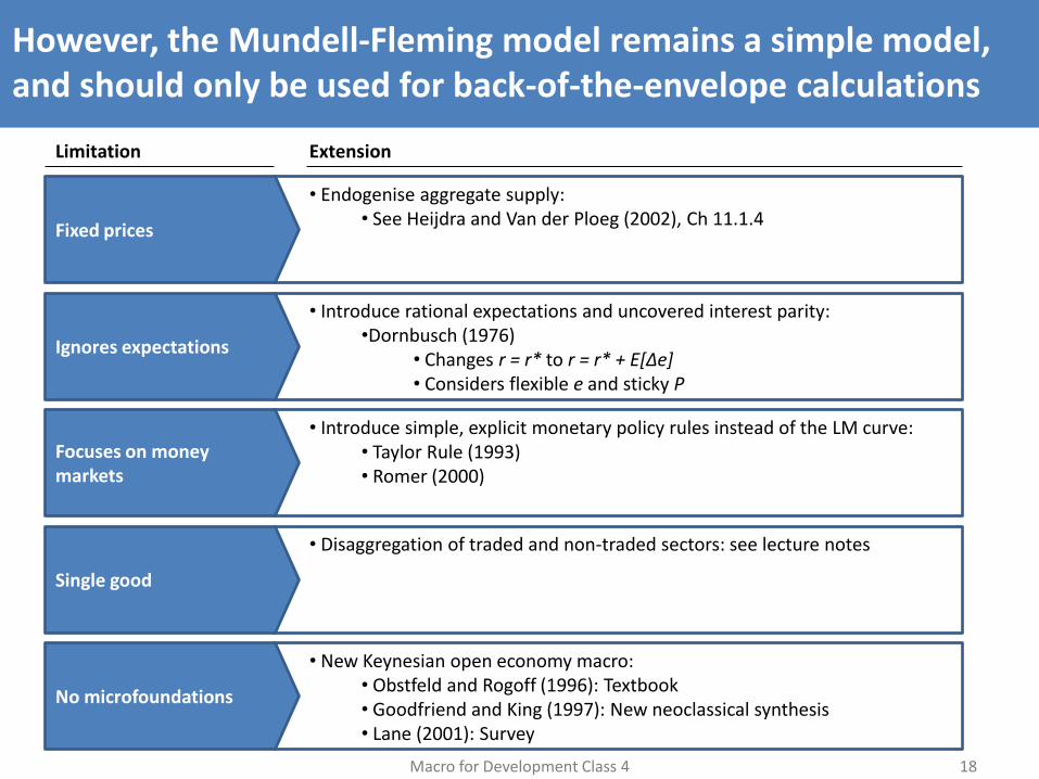
However, the Mundell-Fleming model remains a simple model, and should only be used for back-of-the-envelope calculations
Macro for Development Class 4 18
Fixed prices
• Endogenise aggregate supply: • See Heijdra and Van der Ploeg (2002), Ch 11.1.4
Ignores expectations
• Introduce rational expectations and uncovered interest parity: •Dornbusch (1976)
• Changes r = r* to r = r* + E[Δe] • Considers flexible e and sticky P
Focuses on money markets
• Introduce simple, explicit monetary policy rules instead of the LM curve: • Taylor Rule (1993) • Romer (2000)
Single good
• Disaggregation of traded and non-traded sectors: see lecture notes
No microfoundations
• New Keynesian open economy macro: • Obstfeld and Rogoff (1996): Textbook • Goodfriend and King (1997): New neoclassical synthesis • Lane (2001): Survey
Limitation Extension
Next week’s class
• Hand back problem sets
• Extended consultation session – bring questions!
Macro for Development Class 4 19