
Macroeconomics Chapter 91 Capital Utilization and Unemployment C h a p t e r 9.
48
Macroeconomics Chapter 9 1 Capital Utilization and Unemployment C h a p t e r 9
-
date post
20-Dec-2015 -
Category
Documents
-
view
218 -
download
1
Transcript of Macroeconomics Chapter 91 Capital Utilization and Unemployment C h a p t e r 9.

Macroeconomics Chapter 9 1
Capital Utilization and Unemployment
C h a p t e r 9
Macroeconomics Chapter 9 2
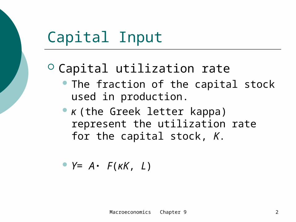
Capital Input
Capital utilization rate The fraction of the capital stock used in
production. κ (the Greek letter kappa) represent
the utilization rate for the capital stock, K.
Y= A· F(κK, L)
Macroeconomics Chapter 9 3
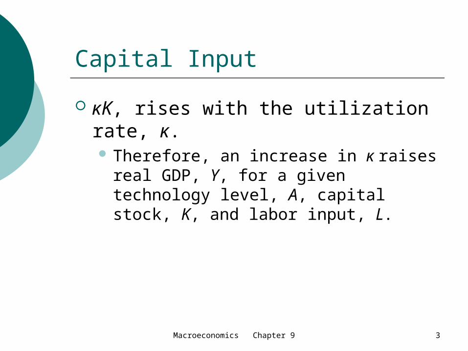
Capital Input
κK, rises with the utilization rate, κ. Therefore, an increase in κ raises real
GDP, Y, for a given technology level, A, capital stock, K, and labor input, L.
Macroeconomics Chapter 9 4
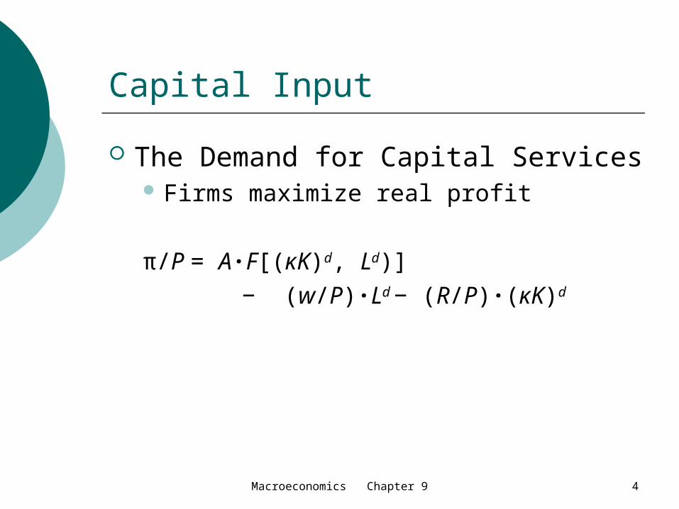
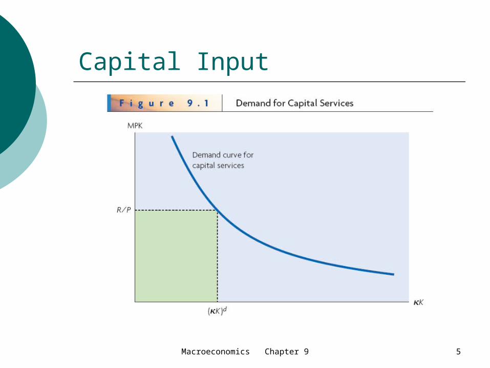
Capital Input
The Demand for Capital Services Firms maximize real profit
π/P = A·F[(κK)d, Ld)] − (w/P)·Ld − (R/P)·(κK)d
Macroeconomics Chapter 9 5
Capital Input

Macroeconomics Chapter 9 6
Capital Input
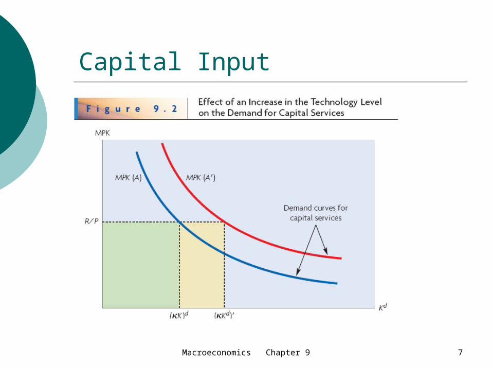
The Demand for Capital Services Assume that the technology level rises
from A to A’. This change raises the MPK at a given quantity.
Macroeconomics Chapter 9 7
Capital Input
Macroeconomics Chapter 9 8
Capital Input
The Supply of Capital Services For a given stock of capital, K, owners can
supply more or less capital services per year by varying κ.
One reason to set the utilization rate, κ, below its maximum is that increases in κ tend to raise the depreciation rate, δ.
δ = δ(κ) Other reasons include utility cost of
capital.
Macroeconomics Chapter 9 9
Capital Input
The Supply of Capital Services Net real income from supplying capital
services = real rental payments − depreciation
= (R/P) · κK − δ(κ) · K = K·[(R/P)·κ − δ(κ)]
Rate of return from owning capital = (R/P)·κ − δ(κ)
Macroeconomics Chapter 9 10
Capital Input
Macroeconomics Chapter 9 11
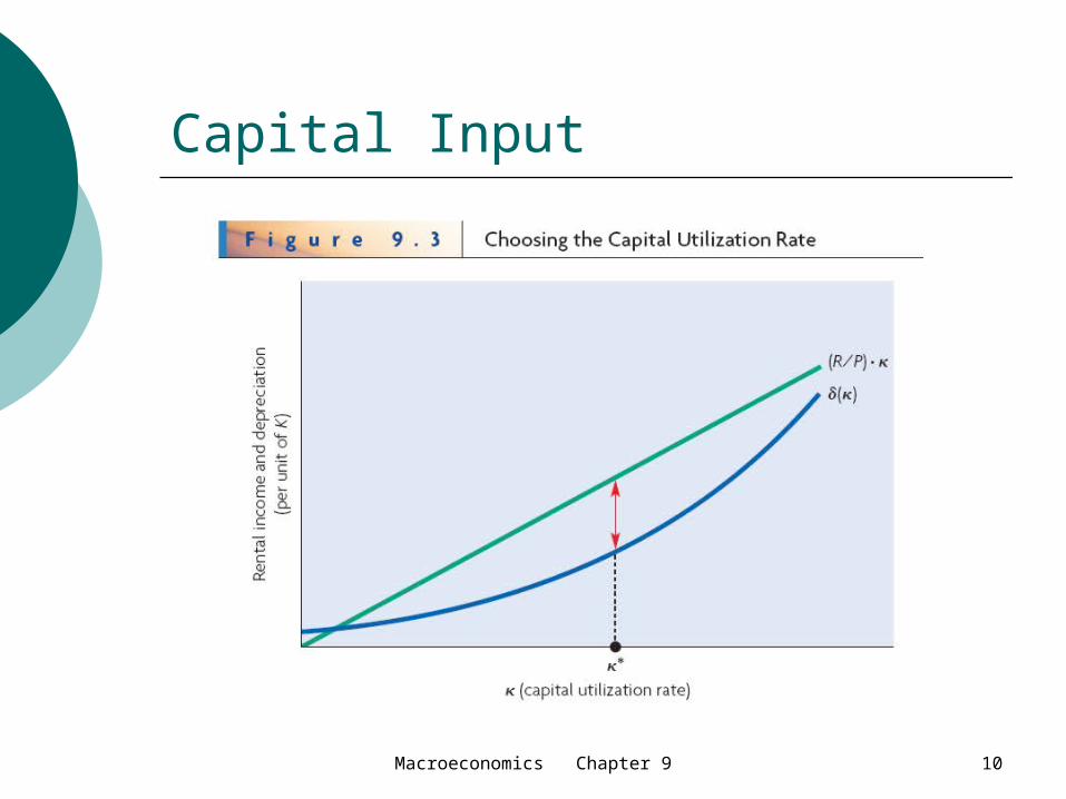
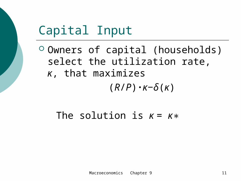
Capital Input Owners of capital (households)
select the utilization rate, κ, that maximizes
(R/P)·κ−δ(κ) The solution is κ = κ∗
Macroeconomics Chapter 9 12
Capital Input
Macroeconomics Chapter 9 13
Capital Input
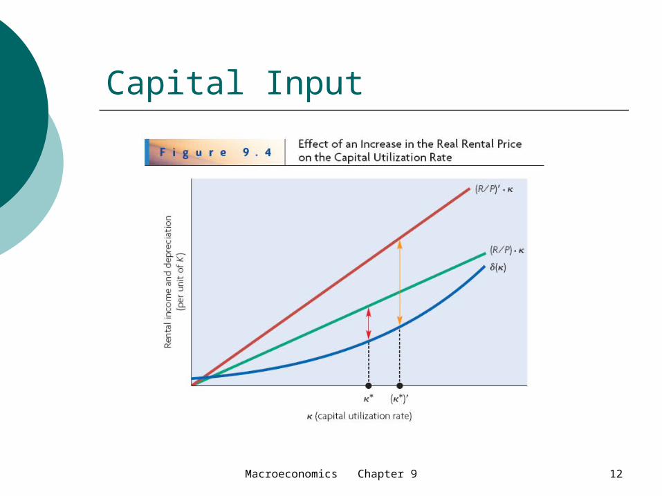
Thus, an increase in the real rental price raises the capital utilization rate; the higher real rental price makes it worthwhile to raise κ despite the resulting increase in the depreciation rate, δ(κ).

Macroeconomics Chapter 9 14
Capital Input
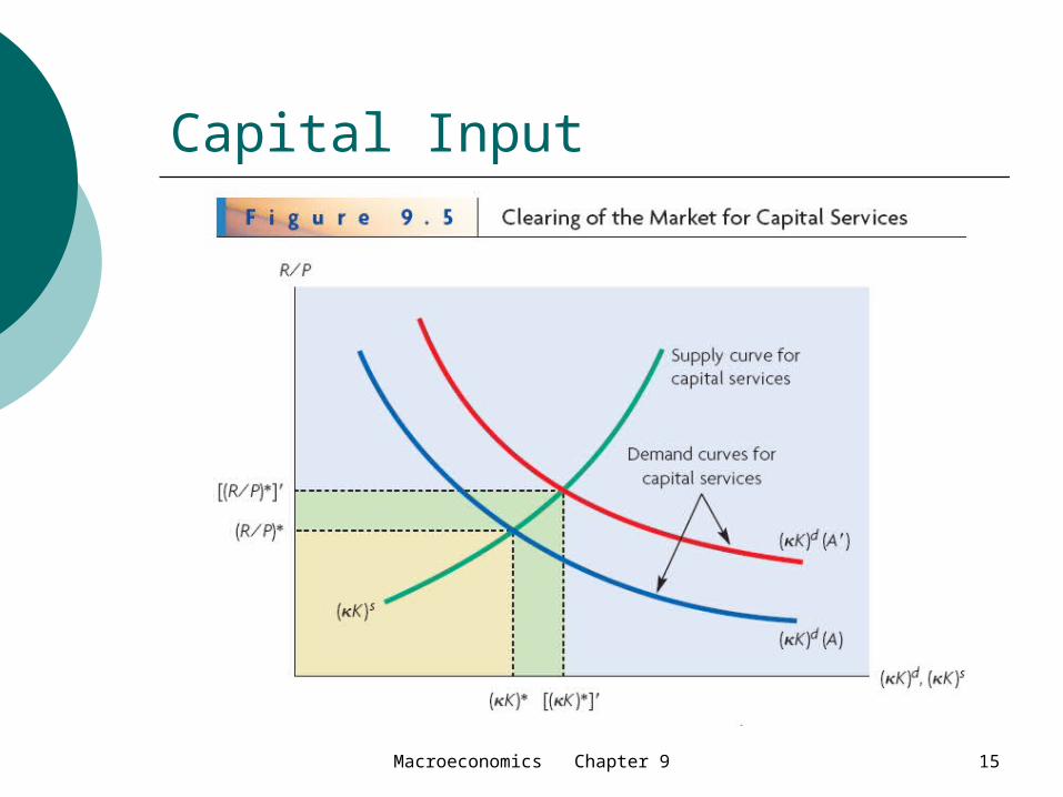
Market Clearing and Capital Utilization
The supply curve slopes up because an increase in the real rental price, R/P, motivates a higher capital utilization rate, κ.
The technology level, A, does not affect the choice of the capital utilization rate, κ
Macroeconomics Chapter 9 15
Capital Input

Macroeconomics Chapter 9 16
Capital Input
Market Clearing and Capital Utilization When the technology level rises to A,
the demand curve for capital services shifts to the right, and the supply curve does not shift.
Therefore the market clears at the higher real rental price, [(R/P)∗], and the larger quantity of capital services, [(κK)∗].
Macroeconomics Chapter 9 17
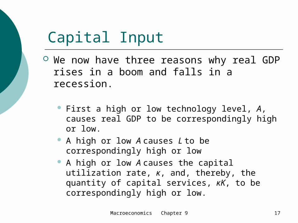
Capital Input We now have three reasons why real GDP
rises in a boom and falls in a recession.
First a high or low technology level, A, causes real GDP to be correspondingly high or low.
A high or low A causes L to be correspondingly high or low
A high or low A causes the capital utilization rate, κ, and, thereby, the quantity of capital services, κK, to be correspondingly high or low.
Macroeconomics Chapter 9 18
Capital Input
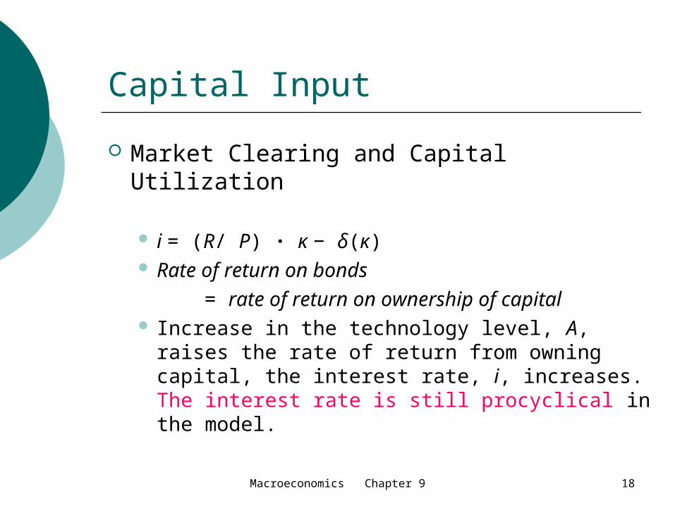
Market Clearing and Capital Utilization
i = (R/ P) · κ − δ(κ) Rate of return on bonds
= rate of return on ownership of capital Increase in the technology level, A, raises
the rate of return from owning capital, the interest rate, i, increases. The interest rate is still procyclical in the model.
Macroeconomics Chapter 9 19
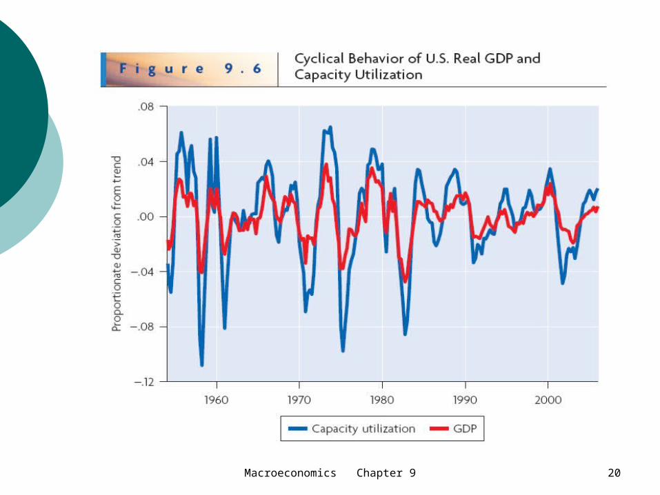
Capital Input The Cyclical Behavior of Capacity
Utilization
The Federal Reserve computes capacity utilization by expressing a sector’s output of goods as a percentage of the estimated “normal capacity” of each sector to produce goods
Macroeconomics Chapter 9 20
Capital Input
Macroeconomics Chapter 9 21
The Labor Force, Employment, and Unemployment
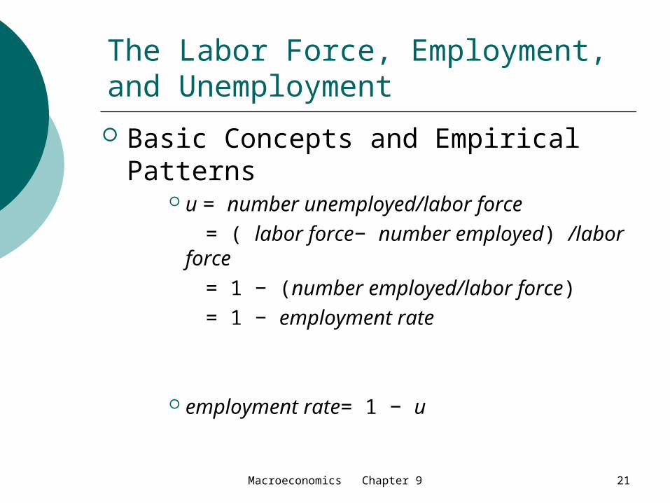
Basic Concepts and Empirical Patterns
u = number unemployed/labor force = ( labor force− number employed) /labor
force = 1 − (number employed/labor force) = 1 − employment rate
employment rate= 1 − u
Macroeconomics Chapter 9 22
The Labor Force, Employment, and Unemployment
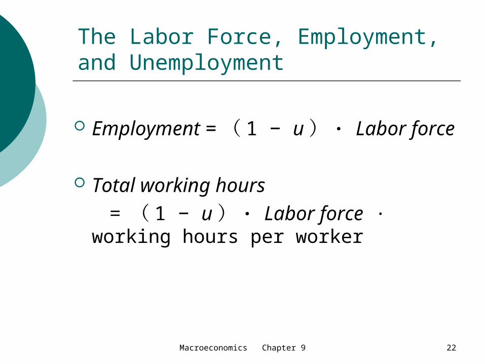
Employment = ( 1 − u ) · Labor force
Total working hours = ( 1 − u ) · Labor force ·
working hours per worker
Macroeconomics Chapter 9 23
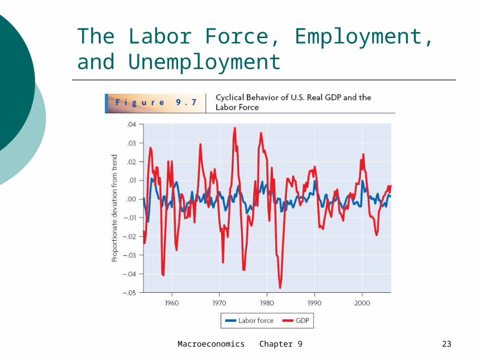
The Labor Force, Employment, and Unemployment
Macroeconomics Chapter 9 24
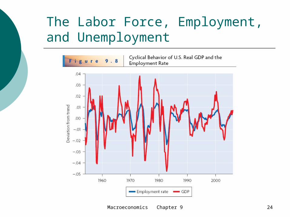
The Labor Force, Employment, and Unemployment
Macroeconomics Chapter 9 25
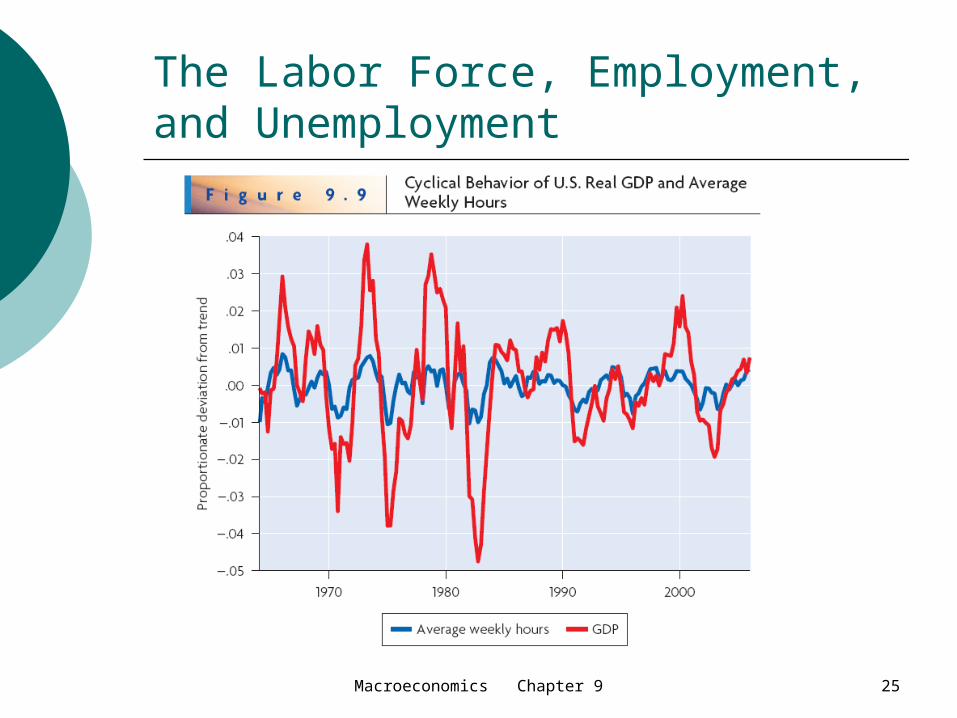
The Labor Force, Employment, and Unemployment
Macroeconomics Chapter 9 26
The Labor Force, Employment, and Unemployment
The equilibrium business-cycle model is probably satisfactory for understanding fluctuations in the labor force and hours worked per worker.
The real wage rate, w/P adjusts to equate the quantity of labor supplied,Ls, to the quantity demanded, Ld.
However, this approach leaves unexplained the most important factor—the fluctuations in the employment rate or, equivalently, in the unemployment rate.

Macroeconomics Chapter 9 27
The Labor Force, Employment, and Unemployment
A Model of Job Finding
Macroeconomics Chapter 9 28
The Labor Force, Employment, and Unemployment
Macroeconomics Chapter 9 29
The Labor Force, Employment, and Unemployment
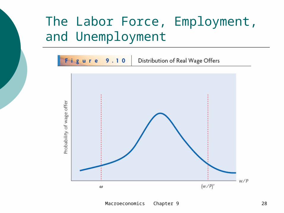
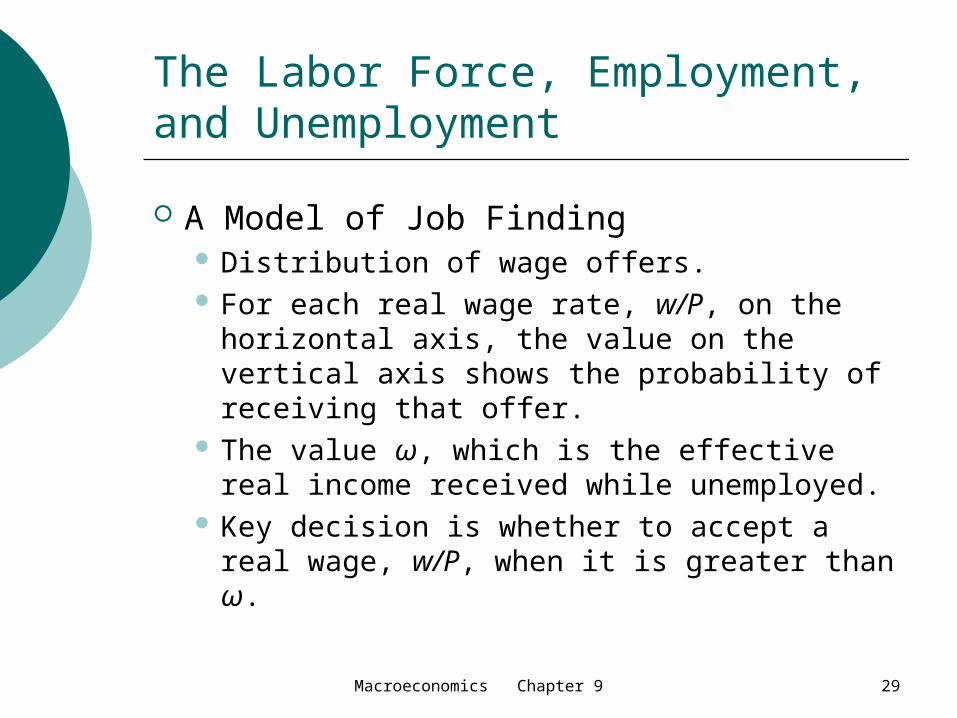
A Model of Job Finding Distribution of wage offers. For each real wage rate, w/P, on the
horizontal axis, the value on the vertical axis shows the probability of receiving that offer.
The value ω, which is the effective real income received while unemployed.
Key decision is whether to accept a real wage, w/P, when it is greater than ω.
Macroeconomics Chapter 9 30
The Labor Force, Employment, and Unemployment
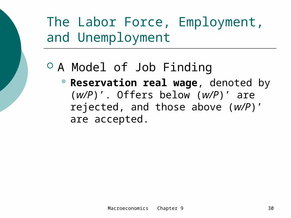
A Model of Job Finding Reservation real wage, denoted by
(w/P)’. Offers below (w/P)’ are rejected, and those above (w/P)’ are accepted.
Macroeconomics Chapter 9 31
The Labor Force, Employment, and Unemployment
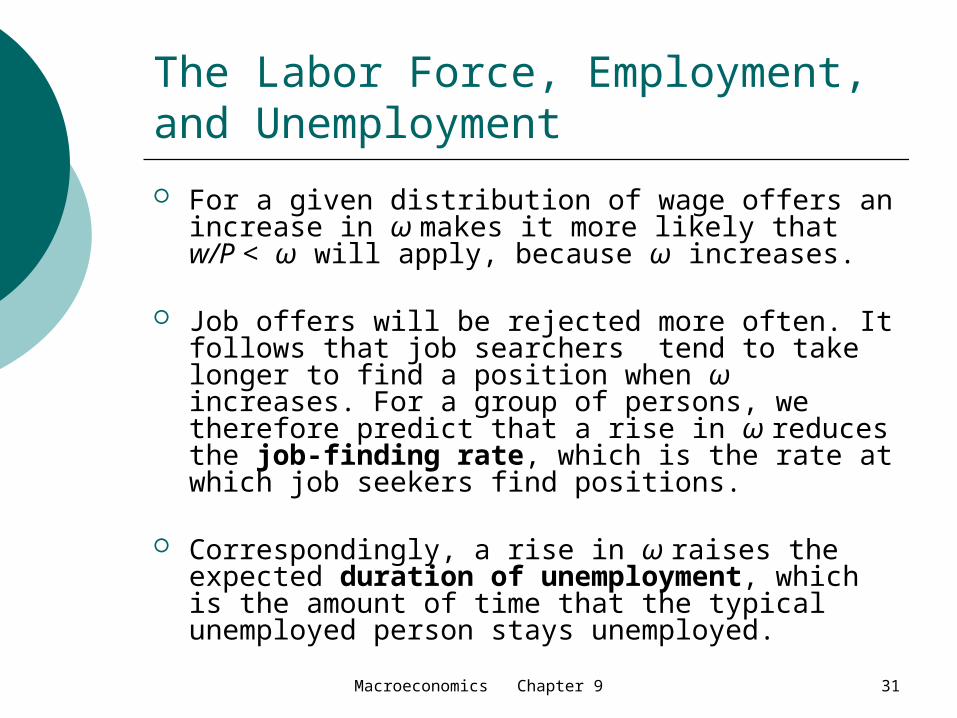
For a given distribution of wage offers an increase in ω makes it more likely that w/P < ω will apply, because ω increases.
Job offers will be rejected more often. It follows that job searchers tend to take longer to find a position when ω increases. For a group of persons, we therefore predict that a rise in ω reduces the job-finding rate, which is the rate at which job seekers find positions.
Correspondingly, a rise in ω raises the expected duration of unemployment, which is the amount of time that the typical unemployed person stays unemployed.
Macroeconomics Chapter 9 32
The Labor Force, Employment, and Unemployment
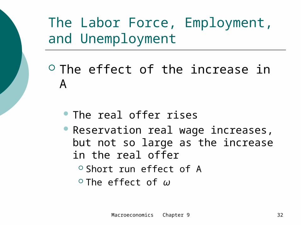
The effect of the increase in A
The real offer rises Reservation real wage increases, but
not so large as the increase in the real offer
Short run effect of A The effect of ω

Macroeconomics Chapter 9 33
The Labor Force, Employment, and Unemployment
Search by Firms is important in a well-functioning labor market, the allowance for this search does not change our major conclusions. It still takes time for workers to match with jobs, so
that the expected durations of unemployment and vacancies are greater than zero.
An increase in workers’ effective real incomes while unemployed, ω, lowers the job-finding rate and raises the expected duration of unemployment.
A favorable shock to productivity raises the job-finding rate and lowers the expected duration of unemployment.
Macroeconomics Chapter 9 34
The Labor Force, Employment, and Unemployment
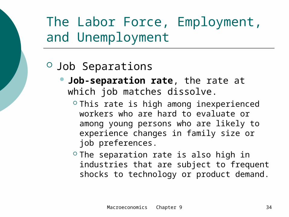
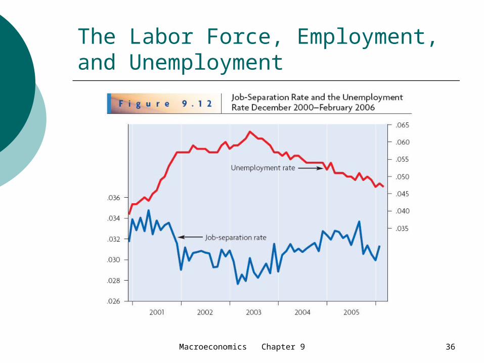
Job Separations Job-separation rate, the rate at which
job matches dissolve. This rate is high among inexperienced
workers who are hard to evaluate or among young persons who are likely to experience changes in family size or job preferences.
The separation rate is also high in industries that are subject to frequent shocks to technology or product demand.

Macroeconomics Chapter 9 35
The Labor Force, Employment, and Unemployment
Job Separations, Job Finding, and the Natural Unemployment Rate
Macroeconomics Chapter 9 36
The Labor Force, Employment, and Unemployment
Macroeconomics Chapter 9 37
The Labor Force, Employment, and Unemployment
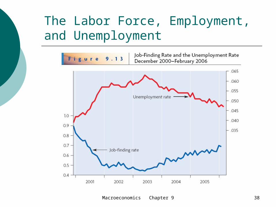
Job Separations, Job Finding, and the Natural Unemployment Rate
Job−finding rate = (number of hires per month) /U
Macroeconomics Chapter 9 38
The Labor Force, Employment, and Unemployment
Macroeconomics Chapter 9 39
The Labor Force, Employment, and Unemployment
Job Separations, Job Finding, and the Natural Unemployment Rate The natural unemployment rate is
the unemployment rate that economy tends towards, given the rates at which people lose and find jobs

Macroeconomics Chapter 9 40
The Labor Force, Employment, and Unemployment
Macroeconomics Chapter 9 41
The Labor Force, Employment, and Unemployment
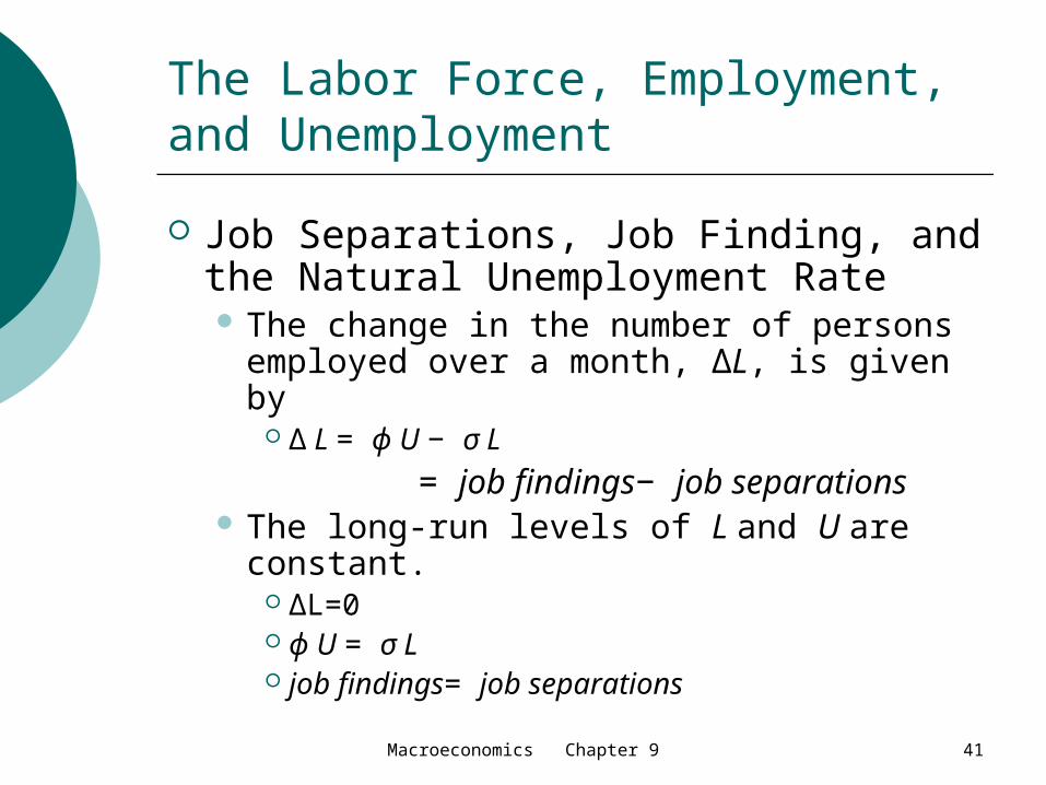
Job Separations, Job Finding, and the Natural Unemployment Rate The change in the number of persons
employed over a month, ∆L, is given by ∆ L = ϕ U − σ L
= job findings− job separations The long-run levels of L and U are
constant. ∆L=0 ϕ U = σ L job findings= job separations
Macroeconomics Chapter 9 42
The Labor Force, Employment, and Unemployment
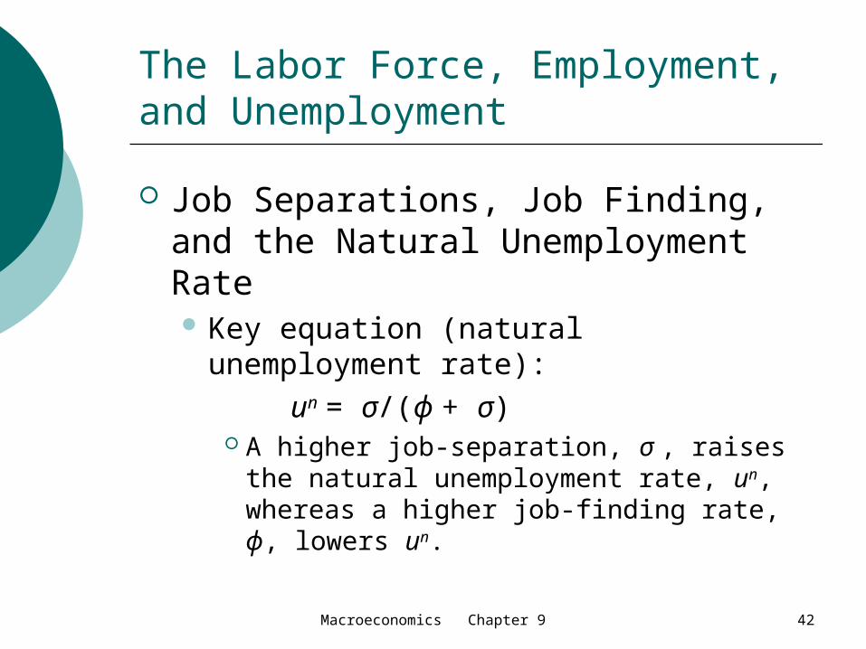
Job Separations, Job Finding, and the Natural Unemployment Rate Key equation (natural unemployment
rate): un = σ/(ϕ + σ)
A higher job-separation, σ , raises the natural unemployment rate, un, whereas a higher job-finding rate, ϕ, lowers un.

Macroeconomics Chapter 9 43
The Labor Force, Employment, and Unemployment
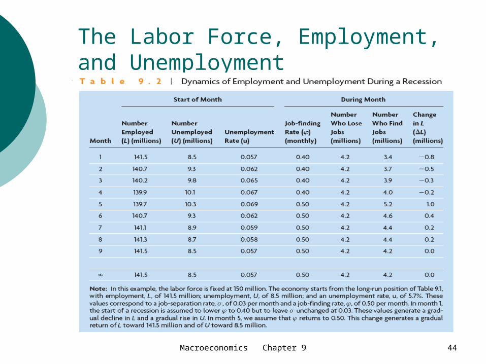
Economic Fluctuations, Employment, and Unemployment An adverse shock to the technology
level, A, reduces the marginal product of labor for the typical worker and job. The job-finding rate, ϕ, falls because market opportunities became poorer—probably temporarily—relative to the real income received while unemployed, ω.
Macroeconomics Chapter 9 44
The Labor Force, Employment, and Unemployment
Macroeconomics Chapter 9 45
The Labor Force, Employment, and Unemployment
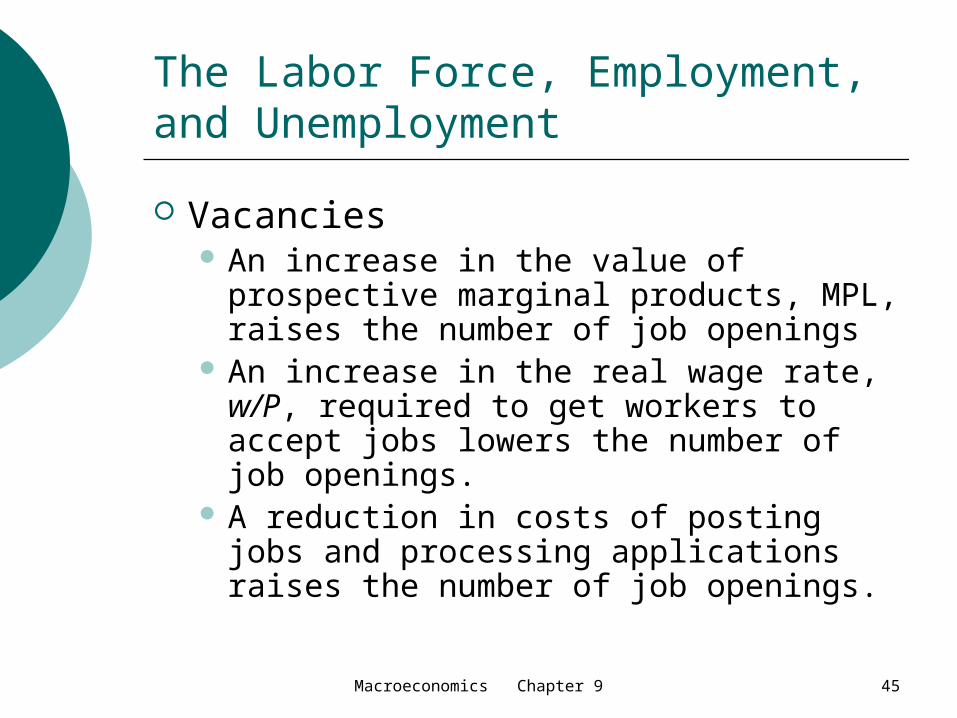
Vacancies An increase in the value of prospective
marginal products, MPL, raises the number of job openings
An increase in the real wage rate, w/P, required to get workers to accept jobs lowers the number of job openings.
A reduction in costs of posting jobs and processing applications raises the number of job openings.
Macroeconomics Chapter 9 46
The Labor Force, Employment, and Unemployment
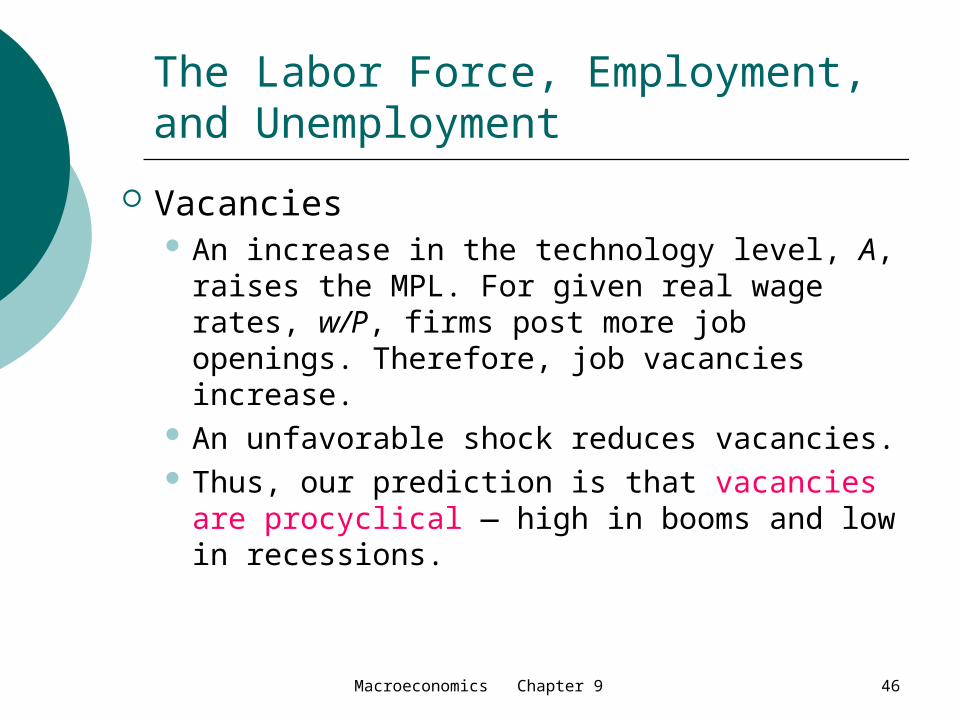
Vacancies An increase in the technology level, A,
raises the MPL. For given real wage rates, w/P, firms post more job openings. Therefore, job vacancies increase.
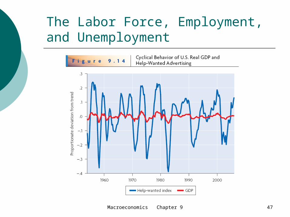
An unfavorable shock reduces vacancies. Thus, our prediction is that vacancies are
procyclical — high in booms and low in recessions.
Macroeconomics Chapter 9 47
The Labor Force, Employment, and Unemployment
Macroeconomics Chapter 9 48
The Labor Force, Employment, and Unemployment


![[spa] Empleo y paro : 1987 [dan] Beskæftigelse og ...aei.pitt.edu/75993/1/1987.pdfΑΠΑΣΧΟΛΗΣΗ KAI ΑΝΕΡΓΙΑ EMPLOYMENT AND UNEMPLOYMENT EMPLOI ET CHÔMAGE OCCUPAZIONE](https://static.fdocument.org/doc/165x107/5ee2c552ad6a402d666d0cd7/spa-empleo-y-paro-1987-dan-beskftigelse-og-aeipittedu7599311987pdf.jpg)