Introducing a Relativistic Nonlinear Field System With a Single

Stable Non-Topological Soliton Solution in 1 + 1 Dimensions

M. Mohammadi∗

Physics Department, Persian Gulf University, Bushehr, 75169, Iran.∗

(Dated: March 6, 2020)

Abstract

In this paper we present a new extended complex nonlinear Klein-Gordon Lagrangian density,

which bears a single non-topological soliton solution with a specific rest frequency ωs in 1 + 1

dimensions. There is a proper term in the new Lagrangian density, which behaves like a massless

spook that surrounds the single soliton solution and opposes any internal changes. In other words,

any arbitrary variation in the single soliton solution leads to an increase in the total energy.

Moreover, just for the single soliton solution, the general dynamical equations are reduced to those

versions of a special type of the standard well-known complex nonlinear Klein-Gordon systems, as

its dominant dynamical equations.

∗ physmohammadi@pgu.ac.ir

1

arX

iv:1

811.

0608

8v5

[ph

ysic

s.cl

ass-

ph]

5 M

ar 2

020

Keywords : solitary wave, Non-topological soliton, energetically stability, massless

spook, Klein-Gordon, Q-ball.

I. INTRODUCTION

Study of soliton solutions in relativistic classical field theories is an attempt to model

particles in terms of non-singular, localized solutions of properly tailored nonlinear PDEs

[1–5]. Kink and anti-kink solutions of the real nonlinear Klein-Gordon (KG) equations in

1 + 1 dimensions were a successful effort to this end [6–40]. In this context, the recent

interesting and important results on kink-(anti)kink interactions in models which possess

kinks with power-law tails (power-law asymptotical behavior of the kink solutions), can be

mentioned [31–35]. Moreover, in the context of kinks and their interactions it is also worth

to mention recent results on the φ8 and more complex models [36–40]. Solitons are, in

some respects, similar to physical particles. They satisfy the relativistic energy-rest mass-

momentum relation and are stable objects. Stability is the main condition for a solitary

wave solution to be a soliton1. As regards stability, there are many different criteria. The

first and foremost criterion is to examine whether a solitary wave solution is topological

or non-topological. Basically, the topological solitary wave solutions are inevitably stable,

among which, one can mention the kink (anti-kink) solutions [6–40] and magnetic monopole

solitons of ’t Hooft Polyakov model [1, 5, 41–43] and solitons of the Skyrme’s model [5, 44–47]

For the non-topological solitary wave solutions, a known standard stability criterion

(method) is the Vakhitov-Kolokolov (or the classical) criterion, which involves obtaining

the permissible small solutions of the linearized equations of motion above the background

of the solitary wave solutions [48–54]. In this method, we first consider any permissible

small perturbation as a localized oscillatory function, as an ansatz, with a specific frequency

ω, and then try to find the possible eigenfunctions and eigenfrequencies. If we find an

eigenfunction with a pure imaginary eigenfrequency ω, or any growing mode, then the soli-

tary wave solution is unstable. If this criterion is used for the topological kink (anti-kink)

solutions, the existence of the non-trivial internal modes would be possible for some kink

1 According to some well-known references such as [1], the stability is just a necessary condition for a solitary

wave solution to be a soliton; more precisely, a solitary wave solution is a soliton if it reappears without

any distortion after collisions. In this paper, we only accept the stability condition for the definition of a

soliton solution.

2

solutions, which causes such kinks (anti-kink) to display a permanent vibrational behavior

in a collision process [6, 10–14]. Moreover, for the non-topological solitary wave solutions of

the real one-field nonlinear Klein-Gordon systems, this criterion leads us to conclude that

there are not any stable solution at all [51].

For the complex nonlinear Klein-Gordon (CNKG) systems, it was shown that there are

some non-topological solutions that are called Q-balls [51–65]. In fact, they are some solitary

wave profiles, which can be identified with their specific rest frequencies ωo. In general, it was

shown that Q-balls have the minimum rest energy among the other solutions with the same

electrical charge [54, 56]. Based on the Vakhitov-Kolokolov stability criterion, the stability

conditions of the Q-balls were obtained in detail [50–54]. Moreover, some researchers have

tried to examine the stability of such non-topological solutions according to the paradigm of

the quantum mechanics [54, 55], which leads to the quantum mechanical stability criterion.

It is based on a comparing between the properties of the Q-ball (such as charge and rest

energy) and the properties of the free scalar particle quanta. A Q-ball which is quantum-

mechanically stable can not decay to a number of free quanta.

In this paper we use a new criterion (i.e. the energetically stability criterion [66–68]) for

the relativistic field systems with the non-topological solitary wave solutions. We assume

that a non-topological solitary wave solution is stable if any arbitrary deformation in its

internal structure, when it is at rest, leads to an increase in the related total energy. In other

words, we assume that a stable solitary wave solution has the minimum energy among the

other close solutions. According to this new criterion, we will show that none of the Q-balls

are stable objects. It should be noted that, this new criterion is different from the Vakhitov-

Kolokolov criterion, but both are classical. Based on the Vakhitov-Kolokolov method, we

examine the dynamical equations of motion for the small oscillations above the background

of the solitary wave solutions (and linearized them to obtain another eigenvalue equation

for the permissible small perturbations). However, the new stability criterion is based on

examining the energy density functional for any arbitrary (permissible or impermissible)

small variation above the background of the solitary wave solutions. This criterion was used

without naming in Derrick’s article [66] about the nonexistent of the stable non-vibrational

solitary wave solutions of the nonlinear Klein-Gordon field systems in 3 + 1 dimensions.

In general, a solitary wave solution which is stable according to the new criterion of the

stability can be called an energetically stable soliton solution.

3

Our main goal in this paper is to find a relativistic complex nonlinear field system that

has just a single stable non-topological solitary wave solution (a single Q-ball solution).

We expect, just for this single solitary wave solution, the general dynamical equations and

other properties be reduced to those versions of a special type of the standard well-known

CNKG systems. We have borrowed this expectation from the quantum field theory at which

any standard (nonlinear) Klein-Gordon (-like) system is used just to describe a special type

of the known particles. It should be noted that, for the known CNKG systems [51–65],

in general, there are infinite solitary wave solutions with different rest frequencies ωo, but

this new system (which we call it extended CNKG system [67–69]) has just a single solitary

wave solution with a specific rest frequency ωs for which the general dynamical equations are

reduced to the same standard CNKG versions, as we expected. In other words, the simple

CNKG system is a special case of the general extended CNKG system which is obtained

just for the single solitary wave solution. Furthermore, we expect it to be a stable solution

according to the new stability criterion which has been introduced in this paper; that is,

we expect its energy to be the minimum among the other (close) solutions. Nevertheless,

for the single solitary wave solution, introduced in this paper, we will show that it is also a

stable solution according to the Vakhitov-Kolokolov and the quantum mechanical stability

criteria of the Q-balls.

To achieve these goals, we add a new proper term to the original CNKG Lagrangian

density in such away that it and all its derivatives will be equal to zero simultaneously just

for the single solitary wave solution. This new proper additional term behaves like a massless

spook2 which surrounds the particle and resists any arbitrary deformations. There are some

parameters Ai’s and Bi’s (i = 1, 2, 3) in the new additional term, whose larger values result

in more stability of the single solitary wave solution. In other words, the larger the values

the greater will be the increase in the total energy for any arbitrary small variation above

the background of the single solitary wave solution. The additional term, just makes the

single solitary wave solution stable and does not appear in any of the observable, meaning

that, it acts like a stability catalyser. In fact, this model shows how we can have a nonlinear

field system with a single stable non-topological solitary wave solution as a rigid particle,

for which the dominant dynamical equations are a special type of the standard CNKG

2 We chose the word ”spook” in order to avoid any confusion with words such as ”ghost” and ”phantom”,

which have their own particular meanings in the literature.

4

equations.

Furthermore, it is necessary to say that the most important motivation for writing this

paper is the existence of several concerns about the fundamental understanding of particles

in quantum theory. In general, quantum mechanics and quantum field theory only describe

the probabilistic behavior of tiny particles under the influence of other particles and environ-

mental factors. However, despite the undeniable successes of quantum theory, our knowledge

of the fundamental particles is still scarce and there are still many unanswered questions

about them. For example, why are there few fundamental particles with specific masses,

charges and other specific properties in nature? Why is the Planck constant ~ the same for

all particles in the universe? Why are some fundamental particles, such as muons, strange

quarks, essentially unstable? Here and in the upcoming works, we do not claim that our

models answer all these questions and describe real particles properly. But, trying to answer

these questions has motivated us to develop a series of new mathematical tools first, and

this article is an important step in this direction.

This paper has been organized as follows: Basic equations and general properties of the

CNKG systems with their solitary wave solutions (Q-balls) are first considered. In the next

section, a new self-interaction potential and the corresponding localized wave solutions will

be considered in detail, together with a stability analysis. In section IV, we will show how

to build an extended CNKG system with a single stable solitary wave solution for which

the general dynamical equations are reduced to a standard CNKG equation. In section V,

the stability of the single soliton solution against any arbitrary small deformations will be

studied according to the new criterion. In section VI, we provide a brief discussion about the

collisions of the single solitary wave solutions with each other. The last section is devoted

to summary and conclusions. It should be note that, this work is in line with [67, 68], but

with more details and accuracy.

II. COMPLEX NONLINEAR KLEIN-GORDON (CNKG) SYSTEMS

The complex nonlinear Klein-Gordon (CNKG) systems in 1 + 1 dimensions can be intro-

duced by the following relativistic Lagrangian-density:

Lo = ∂µφ∗∂µφ− V (|φ|), (1)

5

in which φ is a complex scalar field and V (|φ|) is the self-interaction potential, which depends

only on the modulus of the scalar field. Using the least action principle, the dynamical

equation for the evolution of φ can be obtained as follows:

2φ =∂2φ

∂t2− ∂2φ

∂x2= − ∂V

∂φ∗= −1

2V ′(|φ|) φ

|φ|. (2)

Note that we have used natural units ~ = c = 1 in this paper. For further applications, it is

better to use polar fields R(x, t) and θ(x, t) as defined by

φ(x, t) = R(x, t) exp[iθ(x, t)]. (3)

In terms of polar fields, the Lagrangian-density (1) and related field equation (2) are reduced

respectively to

Lo = (∂µR∂µR) +R2(∂µθ∂µθ)− V (R), (4)

and

2R−R(∂µθ∂µθ) = −1

2

dV

dR, (5)

∂µ(R2∂µθ) = 2R(∂µR∂µθ) +R2(∂µ∂µθ) = 0. (6)

The related Hamiltonian (energy) density is obtained via the Noether’s theorem:

T 00 = ε(x, t) = φφ∗ + φφ∗ + V (|φ|)

= R2 + R2 +R2(θ2 + θ2) + V (R), (7)

in which dot and prime denote differentiation with respect to t and x, respectively. For such

systems, it is possible to have some traveling solitary wave solutions (Q-balls) as follows:

R(x, t) = R(γ(x− vt)), θ(x, t) = kµxµ = ωt− kx, (8)

provided

k = ωv, (9)

and

2R = −d2R

dx2= −1

2

dV

dR+ ω2

oR, (10)

where γ = 1/√

1− v2 and x = γ(x−vt). Note that kµ ≡ (ω, k) is a 1+ 1 dimensional vector

and ∂µθ∂µθ = kµkµ = ω2

o is a constant scalar.

6

If we multiply equation (10) by dRdx

and integrate, it yields(dR(x)

dx

)2

+ ω2oR

2 = V (R) + C, (11)

where C is an integration constant. This constant is expected to vanish for a localized

solitary wave solution. This equation can be easily solved for R, once the potential V (R) is

known:

x− xo = ±∫

dR√V (R)− ω2

oR2, (12)

In general, by using equation (10), it is easy to see that there are different non-topological

solutions for R(x) with different values of ωo. The topological complex kink and anti-kink

solutions can also exist when ωo = 0 and V (R) has more than two vacuum points [65].

In the framework of special relativity, it is clear that the total energy of a solitary wave

solution which represents the total relativistic energy of a particle should read

E =

∫ +∞

−∞ε(x, t)dx = γEo, (13)

in which

Eo =

∫ +∞

−∞[R2 +R2θ2 + V (R)]dx =

∫ +∞

−∞[R2 +R2ω2

o + V (R)]dx, (14)

is the rest energy of a solitary wave solution.

The Lagrangian-density (1) is invariant under global U(1) symmetry. If we link this sym-

metry with electromagnetism, then according to Noether’s theorem, the following electrical

current density is conserved:

jµ ≡ i(φ∂µφ∗ − φ∗∂µφ) = 2R2∂µθ, ∂µjµ = 0. (15)

The corresponding charge is

Q =

∫ +∞

−∞j0dx =

∫ +∞

−∞i(φφ∗ − φ∗φ)dx, (16)

which is a constant of motion.

III. STABILITY CONSIDERATIONS; AN EXAMPLE

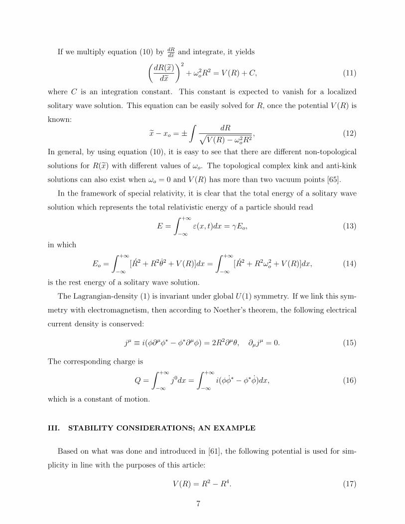
Based on what was done and introduced in [61], the following potential is used for sim-

plicity in line with the purposes of this article:

V (R) = R2 −R4. (17)

7

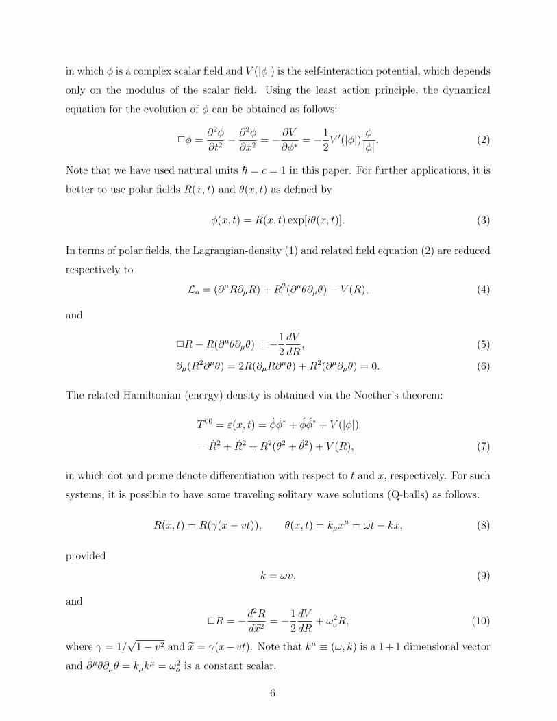
With this potential (17), it can be shown that the integral (12) can be easily performed,

yielding the following solutions for ω− = 0 6 ω2o < 1 = ω+:

R(x) = ω′ sech(ω′x). (18)

where ω′ =√

1− ω2o is called the complementary frequency [61]. Accordingly, there are

infinite solitary wave solutions (18), which can be identified with different rest frequencies

ωo (see Fig. 1). Using Eqs. (14) and (16) for profile functions (18), then one can obtain the

rest energies and total charges:

Eo =4ω′

3(1 + 2ω2

o), Q = 4ωoω′. (19)

Traditionally there are two types of criteria for the stability of the Q-balls. First, the

quantum mechanical criterion [54, 55], which specifies that if the ratio between the rest

energy and the charge is less than ω+ (i.e. Eo/Q < ω+) for a Q-ball solution, it can not

decay to the free scalar particle quanta with a specific rest mass equal to ω+. Second,

the classical criterion [50–54], which is based on examining the permissible small oscillating

perturbations above the background of the Q-balls (not any arbitrary small deformations),

it says that a Q-ball is stable if dQdωo

< 0. Now, if these stability criteria are used for the

system (17) with the Q-ball solutions (18), then it is easy to show that the Q-balls (18)

for which 12< ωo ≤ 1 ( 1√

2= ωc < ωo ≤ 1) are quantum mechanically (classically) stable.

Note that, for the case ωc = 1√2, the maximum value of the related module function is

Rmax = Rωc(0) = 1√2

which is exactly the same turning point of the potential (17) (see

Fig. 2). In general, for any arbitrary solution (18), it is obvious that the solutions for which

Rmax >1√2

are essentially unstable. There is another type of stability called fission stability.

A Q-ball which does not fulfill the requirement of the fission stability, it naturally decays

into two or more smaller Q-balls with some release of energy. In general, it was shown that

the condition of the classical stability of the Q-balls is identical to the condition of fission

stability [54]. Therefore, the Q-balls for which dQdωo

< 0 are stable against fission too.

However, in this paper we use another rigorous criterion for the stability (i.e. the en-

ergetically stability criterion [66–68]). The rest energy of an energetically stable solitary

wave solution is at the minimum among the other (close) solutions. In fact, if the total

energy always increases for any arbitrary (permissible or impermissible) deformation above

the background of a special solitary wave solution which is at rest, it is an energetically

8

FIG. 1. Related to different ω2o ’s, there are different solutions for R(x).

FIG. 2. The field potential (17) versus R

stable solution. Based on this criterion, it is easy to show that there is no stable solitary

wave solution for the CNKG systems in 1 + 1 dimensions at all. For example, for a Q-ball

solution, an arbitrary deformation (variation) can be constructed as follows: according to

Eq. (14), let us fix the function R(x) and set θ = 0, then any small variation in θ2 with

δθ2 < 0, yields a small reduction in the related total energy (14). Therefore, none of the

solitary wave solutions (18) are energetically stable at all. The same argument applies for

the possible non-topological solutions of the real nonlinear KG systems in 1 + 1 dimensions.

Moreover, based on the newly defined stability criterion, a primary condition for a special

solitary wave solution (18) to be a soliton, is that its rest energy must be at the minimum

9

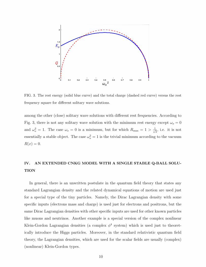
FIG. 3. The rest energy (solid blue curve) and the total charge (dashed red curve) versus the rest

frequency square for different solitary wave solutions.

among the other (close) solitary wave solutions with different rest frequencies. According to

Fig. 3, there is not any solitary wave solution with the minimum rest energy except ωo = 0

and ω2o = 1. The case ωo = 0 is a minimum, but for which Rmax = 1 > 1√

2, i.e. it is not

essentially a stable object. The case ω2o = 1 is the trivial minimum according to the vacuum

R(x) = 0.

IV. AN EXTENDED CNKG MODEL WITH A SINGLE STABLE Q-BALL SOLU-

TION

In general, there is an unwritten postulate in the quantum field theory that states any

standard Lagrangian density and the related dynamical equations of motion are used just

for a special type of the tiny particles. Namely, the Dirac Lagrangian density with some

specific inputs (electrons mass and charge) is used just for electrons and positrons, but the

same Dirac Lagrangian densities with other specific inputs are used for other known particles

like muons and neutrinos. Another example is a special version of the complex nonlinear

Klein-Gordon Lagrangian densities (a complex φ4 system) which is used just to theoret-

ically introduce the Higgs particles. Moreover, in the standard relativistic quantum field

theory, the Lagrangian densities, which are used for the scalar fields are usually (complex)

(nonlinear) Klein-Gordon types.

10

In light of the above, first we postulate that for the soliton solutions (as the particle-

like objects) of the classical scalar field models, the dominant Lagrangian densities (or the

dominant dynamical equations) should be the same standard (complex) (nonlinear) Klein-

Gordon types. Second, if a classical Lagrangian density leads to more than one soliton

solution with the same standard dominant dynamical equations, we postulate that it is not

a physical case. For example, the pervious Lagrangian density (4) with the potential (17)

is not a physical case, because it leads to infinite soliton-like solutions (18) according to

infinite particle-like objects for which the dominant Lagrangian density (4) or the dominant

dynamical equations (5) and (6) are the same. Note that, we used ”soliton-like” instead of

”soliton”, because, according to the new criterion of the stability, essentially none of them

(18) are energetically stable soliton solutions. So far, according to the new criterion of the

stability, no classical field system has been introduced that leads to a non-topological stable

soliton solution. However, we will introduce a new field system in the following. In fact,

the topological property for many soliton solutions is considered to guarantee the stability

automatically and inevitably. The topological property of a soliton solution imposes difficult

conditions for constructing multi-particle solutions. But with non-topological solutions, they

simply result in multi-particle solutions just by adding them when they are sufficiently far

apart.

To meet all these requirements, one can assume that there is an extended complex nonlin-

ear Klein-Gordon (CNKG) Lagrangian density [67–69], which is reduced to a simple standard

CNKG form just for a special soliton solution. Briefly, we are going to consider the possi-

bility of the existence of a new extended CNKG system with a single stable solitary wave

solution, according to the new criterion of the stability, for which the complicated general

dynamical equations are reduced to the same standard CNKG versions (5) and (6) as we

expected. Note that, unlike the quantum field theory, the particle concept in the classical

field theory is completely objective (i.e. a stable localized energy density in the space which

can move in any arbitrary direction).

To make it more objective, we can imagine that a stable solitary wave solution of an

unknown relativistic field system with a specific rest frequency ωs = 0.8 exists in following

11

form:

φs(x, t) = Rs(γ(x− vt)) exp (ikµxµ) = Rs(x) exp (iγωs(t− vx))

= ω′s sech(ω′sx) exp (iωst ), (20)

in which t = γ(t−vx) and ω′s = 0.6. In other words, it is considered to be one of the Q-balls

(18) which is quantum mechanically and classically stable. We can consider this special

solitary wave solution (SSWS) (20) like a detected stable tiny particle in the laboratory for

which we suppose that the dominant dynamical equations of motion or the dominant La-

grangian density be the same standard versions of the CNKG system which were introduced

in the previous sections. In other words, we assume that the dynamical equations of the

system have a general complicated form, and just for the SSWS (20) are reduced to the

same simple standard CNKG forms (5) and (6).

Accordingly, one should consider a new Lagrangian density in the following form:

L = Lo + F = [(∂µR∂µR) +R2(∂µθ∂µθ)− V (R)] + F, (21)

in which Lo is the same original CNKG Lagrangian density (4) for which the SSWS (20)

is one of its solutions. According to the standard classical relativistic field theory, the

Lagrangian densities are considered to be functions of the fields themselves and their first

derivatives. In addition, since the Lagrangian densities must be scalar functionals, they

should be functions of the possible allowed scalars. Along with the scalar fields R and θ,

the other basic (simplest) allowed scalars in our model, which are made via the different

possible contractions of the first derivatives of the scalar fields, are ∂µR∂µR, ∂µθ∂

µθ and

∂µR∂µθ. Accordingly, we conclude that the new additional functional F (which is a part of

the new lagrangian density) should be function of all possible allowed scalars R, θ, ∂µR∂µR,

∂µθ∂µθ and ∂µR∂

µθ. To ensure that the electrical charge conservation is satisfied again, the

additional term F must not be function of the phase field θ. The new dynamical equations

of motion for this new extended Lagrangian density (21) are

2R−R(∂µθ∂µθ) +1

2

dV

dR+

1

2

[∂

∂xµ

(∂F

∂(∂µR)

)−(∂F

∂R

)]= 0 (22)

∂µ(R2∂µθ) +1

2

[∂

∂xµ

(∂F

∂(∂µθ)

)]= 0. (23)

Also, the new energy density function is

ε(x, t) =[R2 + R2 +R2(θ2 + θ2) + V (R)

]+

[R∂F

∂R+ θ

∂F

∂θ

]. (24)

12

For the SSWS (20), as we indicated before, we expect all Eqs. (21), (22), (23) and (24) to

be reduced to the same original versions (1), (5), (6) and (7) respectively. In other words,

we expect all additional terms F , ∂∂xµ

(∂F

∂(∂µR)

), ∂∂xµ

(∂F

∂(∂µθ)

), ∂F∂R

, ∂F∂R

and ∂F∂θ

to be zero just

for the SSWS (20). It means that just for the SSWS (20), the general equations of motion

(23) and (24) turn to the same standard equations (4) and (5) respectively.

Therefore, first, we find the standard CNKG Lagrangian density Lo as the dominant

Lagrangian density for the SSWS (20). Second, we try to find the proper additional term

F in such a way that Lo to be the dominant Lagrangian density just for the SSWS (20),

meaning that, the additional term F and its other derivatives simultaneously turn to zero just

for the SSWS (20). And third, we expect this additional term to guarantee the energetically

stability of the SSWS (20), meaning that the rest energy of the SSWS (20) be at a minimum

among the other (close) solutions of the new system (21). Note that, for this new relativistic

field system (21), there is just a single solitary wave solution (Q-ball) (20) with a specific rest

frequency ωs = 0.8, that is, the other Q-balls (18) of the original system (1) with different

rest frequencies are not the solutions of this new system (21) anymore.

Since F and all its derivatives must be zero for the SSWS (20), one can conclude that it

should be a function of powers of Si’s, where Si’s are introduced as the possible independent

scalars which are zero simultaneously for the SSWS (20). As mentioned earlier, in general,

F must be a function of the allowed scalars, on the other hand, F is considered to be a

function of the powers of the Si’s, thus Si’s must be functions of the allowed scalars as well.

Therefore, there are just three basic independent combinations of the allowed scalars, which

would be zero for the SSWS (20) simultaneously as follows:

S1 = ∂µθ∂µθ − ω2

s , (25)

S2 = ∂µR∂µR + V (R)− ω2

sR2, (26)

S3 = ∂µR∂µθ. (27)

It is straightforward to show that these special scalars all are equal to zero for the SSWS

(20). For simplicitys sake, if one considers F as a function of n’th power of Si’s, i.e. F =

13

F (Sn1 ,Sn2 ,Sn3 ), it yields

∂

∂xµ

(∂F

∂(∂µR)

)=

3∑i=1

[n(n− 1)S(n−2)

i

∂Si∂xµ

∂Si∂(∂µR)

∂F

∂Zi+ nS(n−1)

i

∂

∂xµ

(∂Si

∂(∂µR)

∂F

∂Zi

)]∂F

∂R=

3∑i=1

[nS(n−1)

i

∂Si∂R

∂F

∂Zi

]∂

∂xµ

(∂F

∂(∂µθ)

)=

3∑i=1

[n(n− 1)S(n−2)

i

∂Si∂xµ

∂Si∂(∂µθ)

∂F

∂Zi+ nS(n−1)

i

∂

∂xµ

(∂Si

∂(∂µθ)

∂F

∂Zi

)].

where Zi = Sni . It is easy to understand for n ≥ 3, all these relations would be zero for

the SSWS (20) as we expected. Accordingly, one can show that the general form of the

functional F which satisfies all required constraints, can be introduced by a series:

F =∞∑

n3=0

∞∑n2=0

∞∑n1=0

a(n1, n2, n3)Sn11 Sn2

2 Sn33 , (28)

provided (n1 + n2 + n3) ≥ 3. Note that, coefficients a(n1, n2, n3) are also arbitrary well-

defined functional scalars, i.e. they can be again functions of all possible allowed scalars R,

∂µR∂µR, ∂µθ∂

µθ and ∂µR∂µθ (except θ).

The stability conditions impose serious constraints on function F which causes series (28)

to be reduce to special formats. However, again there are many choices which can lead to

a stable SSWS (20). Among them, one can consider the additional term in the following

form:

F =3∑i=1

Aif(Zi), (29)

where Zi = BiKni for which n is any arbitrary odd number larger than 1 (i.e. n = 3, 5, 7, · · · ),

f(Zi) is any arbitrary odd sinh-like function whose odd derivatives are all non-negative at

Zi = 0 (for example f = Zi [67] or f = Z3i ), Ai’s and Bi’s (i = 1, 2, 3) are just some positive

constants, and functionals Ki’s are three independent linear combinations of Si’s as follows:

K1 = R2S1, (30)

K2 = R2S1 + S2, (31)

K3 = R2S1 + S2 + 2RS3, (32)

It is obvious that K1, K2 and K3 are all zero just for the SSWS (20) with the rest frequency

ωs = ±45

= ±0.8. Note that, these special linear combinations of the Si’s in Eqs. (30)-(32)

14

are introduced just in line with the objectives of this paper and are not unique. One can

use other combinations to obtain different systems with different properties.

The energy-density (24) that belongs to the new extended Lagrangian-density (21), for

this special choice (29), turns to

ε(x, t) =[R2 + R2 +R2(θ2 + θ2) + V (R)

]+

3∑i=1

[nAiBiCiKn−1i f ′i − Aif(Zi)

]= εo + ε1 + ε2 + ε3, (33)

where f ′i =df(Zi)

dZi, and

Ci =∂Ki∂θ

θ +∂Ki∂R

R =

2R2θ2 i=1

2(R2 +R2θ2) i=2

2(R +Rθ)2 i=3.

(34)

Note that, Ci’s are positive definite and this property will be used in the further conclusions.

In fact, this main property originates from the proper combination of the Si’s in Eqs. (30)-

(32) to introduce special functionals K1, K2 and K3.

Since f(Zi) is considered an odd sinh-like function, hence it can be shown generally by a

convergent Maclaurin’s series

f(Zi) =∞∑j=0

ajZ2j+1i =

∞∑j=0

ajB2j+1i K2nj+n

i , (35)

where aj’s are all non-negative. It is easy to obtain f ′i (as an even function) in a series

format:

f ′i =df(Zi)

dZi=∞∑j=0

aj(2j + 1)Z2ji =

∞∑j=0

aj(2j + 1)B2ji K

2nji . (36)

Now, functions εi’s (i = 1, 2, 3) in Eq. (33) can be expressed in the following series:

εi =[nAiBiCiKn−1i f ′i − Aif(Zi)

]= Ai

∞∑j=0

ajB2j+1i K2nj+n−1

i Dij, (37)

where Dij = [nCi(2j + 1)−Ki]. Since n is considered as equal to a positive odd number,

the power of Ki’s (i.e. 2nj+n−1) in the Eq. (37) would be always even numbers. Moreover,

since aj > 0, like a sinh function, the terms AiajB2j+1j K2nj+n−1

i in Eq. (37) will be positive

15

definite and are always zero just for the SSWS (20). Now, from Eq. (34), one can easily

calculate coefficients Dij = [nCi(2j + 1)−Ki]:

Dij =

R2[5θ2 + θ2 + ω2

s ] + C1(2jn+ n− 3) i=1

[5R2θ2 + 5R2 +R2θ2 + R2 + U(R)] + C2(2jn+ n− 3), i=2

[5(Rθ + R)2 + (Rθ + R)2 + U(R)] + C3(2jn+ n− 3), i=3

(38)

where U(R) = 2ω2sR

2 − V (R) = R4 + 725R2, which is a non-negative function and bounded

from below. Therefore, since n ≥ 3 and Ci’s are positive definite, we are sure that all terms

in the above relations are positive definite which means that all terms of the series (37)

would be positive definite. In other words, all εi’s (i = 1, 2, 3) are positive definite functions

which are zero just for the SSWS (20) and the vacuum (R = 0) simultaneously.

Since K1, K2 and K3 (or equivalently S1, S2 and S3) are three independent scalars for

two scalar fields R and θ, it is not possible to find a special variation in the SSWS (20)

for which all of Ki’s do not change and stay zero simultaneously. In other words, just for

the SSWS (20) (and the vacuum R = 0), all Ki’s would be zero simultaneously and for

other non-trivial solutions of the extended CNKG system (21), at least one of the Ki’s (Si’s)

would be a non-zero function (see the Appendix A). Therefore, if constants Ai’s or Bi’s are

considered to be large numbers, we expect for other solutions of the new extended system

(21), according to Eq. (37), at least one of εi’s would be a large positive function, and then

the related rest energy would be larger than SSWS rest energy. Accordingly, we expect the

rest energy of the SSWS (20) would be at a minimum among the other solutions, except the

ones which are very close to the vacuum state (R = 0).

To summarize, the odd functions f(Zi) for which the coefficients of the related Maclaurin’s

series (35) are all non-negative (i.e. aj > 0), are the proper functions to guarantee the

stability of the SSWS (20). In fact, for these special odd sinh-like functions f(Zi), the

additional terms of the energy density function (33), i.e. ε1, ε2 and ε3, would be positive

definite functions and all are zero simultaneously just for the SSWS (20). To prove that

the SSWS (20) is genuinely a stable object, we just considered functions εi’s (i = 1, 2, 3)

but we did not consider function εo! In the next section, we will show that theoretically

and numerically for systems with large enough values of Bi’s (or Ai’s), the influence of the

function εo in the stability property is small and negligible.

16

V. STABILITY FOR SMALL DEFORMATIONS

In this section, based on the new criterion of the stability (energetically stability criterion),

we are going to study the variations of the total energy above the background of the SSWS

(20) for small variations. In general, the arbitrary small variations for the non-moving SSWS

(20) can be considered as follows:

R(x, t) = Rs(x) + δR(x, t) and θ(x, t) = θs(t) + δθ(x, t) = ωst+ δθ(x, t), (39)

where δR and δθ (small variations) are any small functions of space-time. The subscript s is

referred to the special solution (20) for which ω2s = 0.8 and Rs(x) = 0.6 sech(0.6x). Now, if

we insert the deformed version of the non-moving SSWS (39) in εo(x, t) and keep the terms

up to the first order of variations, then it yields

εo(x, t) = εos(x) + δεo(x, t) ≈[Rs

2+R2

sω2s + V (Rs)

]+

2

[Rs(δR) +Rs(δR)ω2

s +R2sωs(δθ) +

1

2

dV (Rs)

dRs

(δR)

]. (40)

Note that, for a non-moving SSWS (20), Rs = 0, θs = 0 and θs = ωs = ±√

0.8. Therefore,

δεo can be considered as a linear function of the first order of small variations δR, δR and δθ.

It is obvious that δεo is not necessarily a positive definite function for arbitrary variations.

If one performs the similar procedure for εi’s, they lead to

εi(x, t) = εis(x) + δεi(x, t) = δεi(x, t)

= Ai

∞∑j=0

ajB2j+1i

[(Dijs + δDij)(Kis + δKi)2nj+n−1

](41)

Note that Ki’s for the SSWS (20) would be zero (i.e. Kis = 0). Now, for simplicity, if one

sets n = 3, then

δεi(x, t) = Ai

∞∑j=0

ajB2j+1i

[(Dijs + δDij)(δKi)6j+2

]≈ Aia0BiDi0s(δKi)2, (42)

According to Eq. (34), Di0s = 3Cis −Kis = 3Cis = 6R2sω

2s , then Eq. (42) is simplified to

δεi(x, t) ≈ 6AiBia0R2sω

2s(δKi)2 ∝ AiBi(δKi)2 ≥ 0, (43)

hence, for small variations δεi’s are all positive definite functions as we generally expected.

17

It is easy to show that δKi’s, similar to δεo, are all linear functions of the first order of small

variations. In fact, according to Eqs. (30)-(32) and (25)-(27) we can define three linear func-

tions G1, G2 and G3 in terms of small variations as follows: δK1 = G1(δθ) = 2ωsR2sδθ, δK2 =

G2(δR, δR, δθ) = G1 − 2Rs(δR) + (dV (Rs)dRs

− 2ω2sRs)δR and δK3 = G3(δR, δR, δR, δθ, δθ) =

G2 + 2Rs(ωsδR − Rsδθ) respectively. Hence, from Eq. (43), one can simplify conclude that

δεi (i = 1, 2, 3) is a linear function of the second order of small variations which is multiplied

by coefficient AiBi. In other words, we can define three linear functions W1, W2 and W3 in

such a way that δε1 = A1B1 W1([δθ]2), δε2 = A2B2 W2([δR]2, [δR]2, [δθ]2, δRδR, δRδθ, δRδθ)

and δε3 = A3B3 W3([δR]2, [δR]2, [δR]2, [δθ]2, [δθ]2, δRδR, δRδR, δRδθ, · · · , δθδθ). For small

variations, it is obvious that the magnitude of the first order of variations is larger than the

magnitude of the second order of them (for example, δR < (δR)2), hence, it is easy to un-

derstand that for small variations: Wi < Gi or Wi < δεo (i = 1, 2, 3). But, if constants Ai’s

or Bi’s are considered to be large numbers, the comparison between δεi = AiBiWi and Gi

(or δεo) needs more considerations. For example, if one considers Ai = Bi = 1020, then for

the variations larger (smaller) than δR = 10−10 we have δR < AiBi(δR)2 (δR > AiBi(δR)2),

hence the same argument goes for the comparison between δεi’s and Gi’s or the comparison

between δεi’s and δεo.

Accordingly, if constants Ai’s and Bi’s are not large numbers, it is obvious that |δεo| <∑3i=1 δεi for all small deformations. But, if constants Ai’s and Bi’s are considered to be

large numbers, |δεo| just for too small variations may be larger than∑3

i=1 δεi, and then the

variation of the total energy density may be negative, i.e. it may be δε = δεo+∑3

i=1 δεi < 0.

For such too small variations the stability conditions of the new criterion may not fulfilled;

nevertheless, they are physically too small which can be ignored in stability considerations.

In fact, these too small variations are a sign of the fact that, the dominant dynamical

equations of motion for the SSWS (20) are the same standard original CNKG equations (5)

and (6). Therefore, like a chicken in the egg in which its internal movements are confined

by the egg shell, this SSWS (20) can have some unimportant internal deformations which

are confined by the additional term F in the new system (21).

To summarize, if we consider the extended CNKG systems with large Ai’s or Bi’s, δε

would be always positive for all significant physical variations (δR and δθ) and then the

stability of the SSWS would guaranteed appreciably. Just for some unimportant too small

variations, it may be possible to see the violation of the stability, but the rest energy reduc-

18

tion for these variations are so small that they can be ignored physically. Although, the Ai’s

and Bi’s parameters can be taken as very large values, but they will not affect the dynamical

equations and the other properties of the SSWS (20). In other words, the additional term

F (29) in the new system (21) with large values of parameters Bi’s (or Ai’s) behaves like a

stability catalyser, but does not have any role in the observables of the SSWS (20). In the

following, we will introduce many arbitrary variations and will show numerically how con-

sidering systems with large Ai’s and Bi’s appreciably guarantees the stability of the SSWS

(20).

From now on, according to Eq. (35) and the pervious discussions, let us consider an odd

function in the following form:

f(Zi) = sinh(Zi), (44)

where Zi = BiK3i . Therefore, the related extended Lagrangian density is

L =[∂µR∂µR +R2(∂µθ∂µθ)− V (R)

]+

3∑i=1

Ai sinh(BiK3i ) = Lo + L1 + L2 + L3. (45)

The related equations of motion are[2R−R(∂µθ∂µθ) +

1

2

dV

dR

]+

3∑i=2

[3

2AiBi

∂

∂xµ

(K2i

∂Ki∂(∂µR)

cosh(BiK3i )

)]−

3∑i=2

[3

2AiBi

(K2i

∂Ki∂R

cosh(BiK3i )

)]= 0, (46)

∂µ(R2∂µθ) +2∑i=1

[3

2AiBi

∂

∂xµ

(K2i

∂Ki∂(∂µθ)

cosh(BiK3i )

)]= 0, (47)

and the related energy density is

ε(x, t) =[R2 + R2 +R2(θ2 + θ2) + V (R)

]+[6A1B1R

2θ2K21 cosh(B1K3

1)− A1 sinh(B1K31)]

+[6A2B2(R

2 +R2θ2)K22 cosh(B2K3

2)− A2 sinh(B2K32)]

+[6A3B3(R +Rθ)2K2

3 cosh(B3K33)− A3 sinh(B3K3

3)]

= εo + ε1 + ε2 + ε3. (48)

An arbitrary hypothetical variation for the non-moving SSWS (20) can be introduced as

follows:

R(x) = Rs + δR = 0.6 sech(0.6x) + ξ exp (−x2), θ(t) = ωst, (49)

in which ξ is a small coefficient. Larger ξ is related to larger variations for the modulus

function. We consider the phase function to be fixed at θ(t) = ωst. Now, the total energy

19

density (48) for this variation (49) is reduced to

ε(x, t) =[R2 +R2(ω2

s)−R4 +R3 + 10R2]

+[6A2B2ω

2sR

2K22 cosh(B2K3

2)− A2 sinh(B2K32)]

+[6A3B3ω

2sR

2K23 cosh(B3K3

3)− A3 sinh(B3K33)]. (50)

Note that for this arbitrary variation (49): R = 0, θ2 = ω2s = 0.64, θ = 0 and then

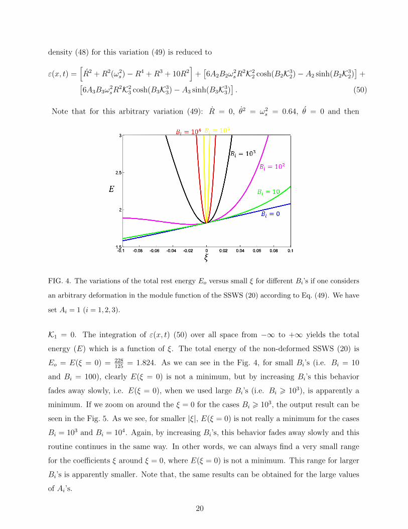
FIG. 4. The variations of the total rest energy Eo versus small ξ for different Bi’s if one considers

an arbitrary deformation in the module function of the SSWS (20) according to Eq. (49). We have

set Ai = 1 (i = 1, 2, 3).

K1 = 0. The integration of ε(x, t) (50) over all space from −∞ to +∞ yields the total

energy (E) which is a function of ξ. The total energy of the non-deformed SSWS (20) is

Eo = E(ξ = 0) = 228125

= 1.824. As we can see in the Fig. 4, for small Bi’s (i.e. Bi = 10

and Bi = 100), clearly E(ξ = 0) is not a minimum, but by increasing Bi’s this behavior

fades away slowly, i.e. E(ξ = 0), when we used large Bi’s (i.e. Bi > 103), is apparently a

minimum. If we zoom on around the ξ = 0 for the cases Bi > 103, the output result can be

seen in the Fig. 5. As we see, for smaller |ξ|, E(ξ = 0) is not really a minimum for the cases

Bi = 103 and Bi = 104. Again, by increasing Bi’s, this behavior fades away slowly and this

routine continues in the same way. In other words, we can always find a very small range

for the coefficients ξ around ξ = 0, where E(ξ = 0) is not a minimum. This range for larger

Bi’s is apparently smaller. Note that, the same results can be obtained for the large values

of Ai’s.

20

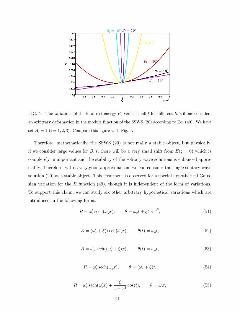
FIG. 5. The variations of the total rest energy Eo versus small ξ for different Bi’s if one considers

an arbitrary deformation in the module function of the SSWS (20) according to Eq. (49). We have

set Ai = 1 (i = 1, 2, 3). Compare this figure with Fig. 4.

Therefore, mathematically, the SSWS (20) is not really a stable object, but physically,

if we consider large values for Bi’s, there will be a very small shift from E(ξ = 0) which is

completely unimportant and the stability of the solitary wave solutions is enhanced appre-

ciably. Therefore, with a very good approximation, we can consider the single solitary wave

solution (20) as a stable object. This treatment is observed for a special hypothetical Gaus-

sian variation for the R function (49), though it is independent of the form of variations.

To support this claim, we can study six other arbitrary hypothetical variations which are

introduced in the following forms:

R = ω′s sech(ω′sx), θ = ωst+ ξt e−x2

, (51)

R = (ω′s + ξ) sech(ω′sx), θ(t) = ωst, (52)

R = ω′s sech((ω′s + ξ)x), θ(t) = ωst, (53)

R = ω′s sech(ω′sx), θ = (ωs + ξ)t, (54)

R = ω′s sech(ω′sx) +ξ

1 + x2cos(t), θ = ωst, (55)

21

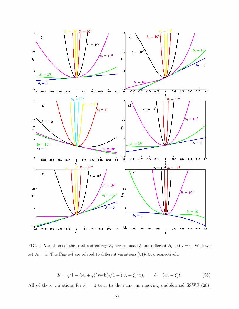
FIG. 6. Variations of the total rest energy Eo versus small ξ and different Bi’s at t = 0. We have

set Ai = 1. The Figs a-f are related to different variations (51)-(56), respectively.

R =√

1− (ωs + ξ)2 sech(√

1− (ωs + ξ)2x), θ = (ωs + ξ)t. (56)

All of these variations for ξ = 0 turn to the same non-moving undeformed SSWS (20).

22

The expected results for the variations of the total energy E versus ξ, for six arbitrary

deformations (51)-(56) at t = 0, are shown in the Fig. 6 respectively. Note that, the case

Bi = 0 is related to the same original standard CNKG system (1) with the potential (17),

and it is quite clear that this case is by no means stable according to the new criterion.

In short, if constants Ai’s and Bi’s are considered to be large numbers, the new additional

term (29) behaves like a zero rest mass spook which surrounds the SSWS (20) and resists

any arbitrary deformation. In fact, it causes to have a frozen or rigid solitary wave solution

(20) for which the modulus and phase functions freeze to R(x, t) = ω′s sech(ω′sγ(x− vt)) and

θ(x, t) = kµxµ = γωs(t − vx), respectively; and the related dominant dynamical equations

are the same known standard versions (5) and (6).

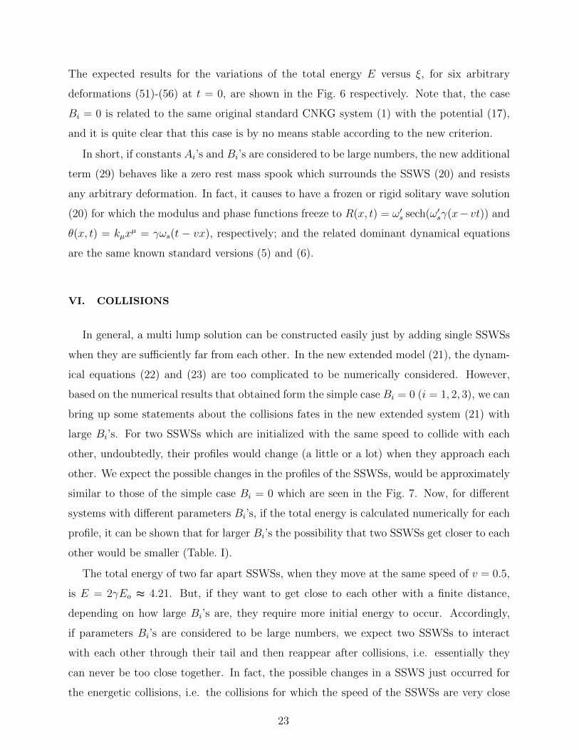
VI. COLLISIONS

In general, a multi lump solution can be constructed easily just by adding single SSWSs

when they are sufficiently far from each other. In the new extended model (21), the dynam-

ical equations (22) and (23) are too complicated to be numerically considered. However,

based on the numerical results that obtained form the simple case Bi = 0 (i = 1, 2, 3), we can

bring up some statements about the collisions fates in the new extended system (21) with

large Bi’s. For two SSWSs which are initialized with the same speed to collide with each

other, undoubtedly, their profiles would change (a little or a lot) when they approach each

other. We expect the possible changes in the profiles of the SSWSs, would be approximately

similar to those of the simple case Bi = 0 which are seen in the Fig. 7. Now, for different

systems with different parameters Bi’s, if the total energy is calculated numerically for each

profile, it can be shown that for larger Bi’s the possibility that two SSWSs get closer to each

other would be smaller (Table. I).

The total energy of two far apart SSWSs, when they move at the same speed of v = 0.5,

is E = 2γEo ≈ 4.21. But, if they want to get close to each other with a finite distance,

depending on how large Bi’s are, they require more initial energy to occur. Accordingly,

if parameters Bi’s are considered to be large numbers, we expect two SSWSs to interact

with each other through their tail and then reappear after collisions, i.e. essentially they

can never be too close together. In fact, the possible changes in a SSWS just occurred for

the energetic collisions, i.e. the collisions for which the speed of the SSWSs are very close

23

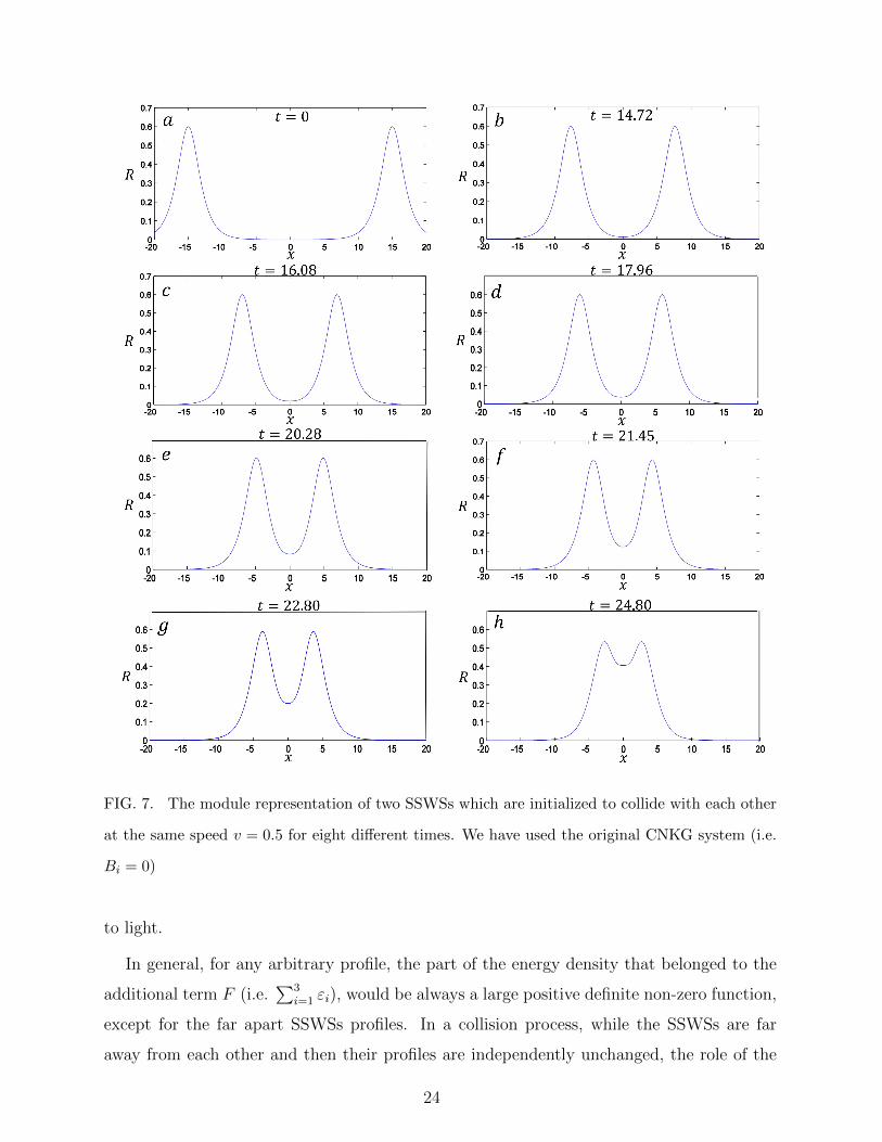
FIG. 7. The module representation of two SSWSs which are initialized to collide with each other

at the same speed v = 0.5 for eight different times. We have used the original CNKG system (i.e.

Bi = 0)

to light.

In general, for any arbitrary profile, the part of the energy density that belonged to the

additional term F (i.e.∑3

i=1 εi), would be always a large positive definite non-zero function,

except for the far apart SSWSs profiles. In a collision process, while the SSWSs are far

away from each other and then their profiles are independently unchanged, the role of the

24

TABLE I. If the various profiles which are shown in the Fig. 7 are considered as the approximations

of the profiles of two SSWSs for other systems (45) with different Bi’s (i = 1, 2, 3), when they

approach each other, they lead to different total energies. We have set Ai = 1.

systemsprofiles

a b c d e f g h

Bi = 108 E ≈ 4.21 E ≈ 10.1 E ≈ 62.9 E ≈ 587 E v 105 E v 1050 E v∞ E v∞

Bi = 107 E ≈ 4.21 E ≈ 4.8 E ≈ 10.1 E ≈ 62.4 E ≈ 604 E v 106 E v 10106 E v∞

Bi = 106 E ≈ 4.21 E ≈ 4.3 E ≈ 4.8 E ≈ 10.0 E ≈ 63.0 E ≈ 637 E v 1012 E v 10256

Bi = 105 E ≈ 4.21 E ≈ 4.21 E ≈ 4.3 E ≈ 4.8 E ≈ 10.1 E ≈ 61.8 E ≈ 1500 E v 1028

Bi = 104 E ≈ 4.21 E ≈ 4.21 E ≈ 4.21 E ≈ 4.3 E ≈ 4.8 E ≈ 10 E ≈ 63.5 E ∼ 104

Bi = 103 E ≈ 4.21 E ≈ 4.21 E ≈ 4.21 E ≈ 4.21 E ≈ 4.21 E ≈ 4.8 E ≈ 10.1 E ≈ 66.5

Bi = 102 E ≈ 4.21 E ≈ 4.21 E ≈ 4.21 E ≈ 4.21 E ≈ 4.21 E ≈ 4.3 E ≈ 4.8 E ≈ 10

Bi = 101 E ≈ 4.21 E ≈ 4.21 E ≈ 4.21 E ≈ 4.21 E ≈ 4.21 E = 4.21 E ≈ 4.3 E ≈ 4.8

Bi = 0 E ≈ 4.21 E ≈ 4.21 E ≈ 4.21 E ≈ 4.21 E ≈ 4.21 E ≈ 4.21 E ≈ 4.21 E ≈ 4.21

spook term F is zero (i.e.∑3

i=1 εi = 0), but when they get close to each other and then

their profiles change slightly, the role of the spook term becomes important and strongly

opposes a closer approach and more changes in the profiles of the SSWSs. For example,

according to Fig. 1 and Table. I, if we consider a system with Bi = 108, to put two SSWSs

at an approximate distance of 10, the initial energy must be in the order of 105 or the initial

speed must be approximately equal to 0.999999999. Therefore, we can be sure that for the

systems with large Bi’s, there is always a huge repulsive force between SSWSs which not

allow two distinct SSWSs to get close together. Hence, we expect they reappear with no

considerable changes after collisions.

If we consider the systems for which parameters Bi’s (or Ai’s) be extremely large numbers,

we can divide the nature of such systems into two distinct stationary parts: first, the vacuum

state, and second, the free far apart SSWSs. Except the free far apart SSWSs and the vacuum

state (R = 0), for other possible stable field solutions (structures), always∑3

i=1 εi would be

a very large positive definite function which yields a very large total energy, then infinite

energy is required for them to be created.

25

VII. SUMMARY AND CONCLUSION

We first reviewed some basic properties of the complex nonlinear KG (CNKG) systems in

1+1 dimensions. Each CNKG system may have some non-dispersive solitary wave solutions

with particular rest frequencies (ωo) and rest energies (Eo), called Q-balls. Traditionally,

two distinct criteria are used to check the stability of the Q-balls: the classical criterion and

the quantum mechanical criterion. In this paper, we used a new criterion for examining

the stability (i.e. the energetically stability criterion) of a solitary wave solution that is

based on examining the changes in the total energy for arbitrary small variations above the

background of the special solitary wave solution. In other words, a special solitary wave

solution is energetically stable, if the total energy, for any arbitrary variation in its internal

structure, always increases. Accordingly, we showed that in general, there is not any CNKG

system with an energetically stable Q-ball solution at all.

Inspire by the well-known quantum field theory in which any standard Lagrangian density

is (nonlinear) Klein-Gordon (-like) and is used just for a special type of known particles with

specific properties, classically we assume that there is a new extended CNKG system with a

single stable solitary wave solution (Q-ball) for which the general dynamical equations (and

the other properties) are reduced to those versions of a standard CNKG system. In fact, we

put forward three basis postulates. First, we assumed a relativistic localized wave function

(20) as a single hypothetical particle of an unknown field model. Second, we assumed that

the dominant dynamical equations of motion just for this special solution (20) are the same

standard known CNKG versions. And eventually we assumed that this special solution (20)

is an energetically stable solution. All of these postulates oblige us to add a proper term F

to the original CNKG Lagrangian density, where it and all of its derivatives should be zero

for this special solitary wave solution (SSWS) (20).

In this regard, it was introduced three independent functional scalars Si (i = 1, 2, 3),

which are zero simultaneously just for the trivial vacuum state R = 0 and a non-trivial

SSWS (20). In other words, the SSWS (20) is the unique non-trivial common solution of

three independent conditions Si’s= 0. The proper additional term F , which is considered

in the new extended CNKG model (21), can be considered in the following form: F =∑3i=1Aif(Zi), where Zi = BiKni , n = 3, 5, 7, · · · , Ai’s and Bi’s are some positive constants,

f is any arbitrary odd sinh-like function, and Ki’s are three special independent linear

26

combinations of Si’s. For such proper additional terms (29), the corresponding energy

density function (33) is decomposed into four distinct parts εi (i = 0, 1, 2, 3). In general, εi’s

(i = 1, 2, 3) are positive definite functions, that any of their terms contains one of the even

powers of Ki’s, and are zero simultaneously just for the non-trivial SSWS (20) and trivial

vacuum state R = 0. Except εo, which originates from the basic standard CNKG system

(1), the other parts of the energy density function, i.e. εi (i = 1, 2, 3), all originate from

the additional term F and all contain parameters Bi’s and Ai’s (i = 1, 2, 3). If parameters

Bi’s and Ai’s are considered to be large numbers, thus εi’s (i = 1, 2, 3) are large functions

in compared with function εo. More precisely, for the other solutions of the system, which

are not very close to the trivial vacuum state R = 0 and non-trivial SSWS (20), always at

least one of the independent functionals Ki’s is not zero, and then at least one of the εi

(i = 1, 2, 3) is a large non-zero positive function. Accordingly, it was shown analytically and

numerically that the SSWS (20) would be approximately an energetically stable solution,

provided Bi’s or Ai’s (i = 1, 2, 3) are considered to be large number. In fact, there are

always very small arbitrary variations above the background of the SSWS (20) for which

the total energy decreases. But, this decreasing is so small that can be physically ignored

in the stability considerations. However, for the other significant small variations, it was

shown that the total energy always increases and the energetically stability of the SSWS

(20) would guaranteed appreciably.

The stability for the SSWS (20) would be intensified by taken into account the larger

values of parameters Bi’s or Ai’s (i = 1, 2, 3) which appeared in the new additional term F .

In other words, the larger the values the greater will be the increase in the total energy for

any arbitrary small variation above the background of SSWS (20). Accordingly, the proper

additional term F (29) behaves like a massless spook which surrounds the single SSWS (20)

and resists any arbitrary significant small deformations in its internal structure. The role

of the additional term F in the collisions behaves like a huge repulsive force which does not

allow two SSWSs to get close each other. Therefore, it is expected that SSWSs reappear

without any distortion in collisions with each other.

If one considers a system for which parameters Bi’s (or Ai’s) be extremely large numbers,

then the other configurations of the fields R and θ, which are not very close to any number

of distinct far apart SSWSs and trivial vacuum state R = 0, require infinite external energy

to be created. In other words, if one considers this system as a real physical system, since it

27

is not possible to provide an extremely large external energy at a special place for creating

the other configurations of the fields R and θ, thus the only non-trivial configurations of

the fields with the finite energies would be any number of the far apart SSWSs as a multi

particle-like solution. Physically this issue can be interesting, in fact it classically explains

how a system leads to many identical particles with the specific characteristics. In fact, the

free far apart SSWSs can be called the quanta of the system classically.

To summarize, this paper introduces an extended CNKG system that yields a single

non-topological energetically stable solitary wave solution for which the general dynamical

equations are reduced to those versions of a special type of the standard well-known CNKG

systems. It is noteworthy to mention, only some relativistic topological solutions such as

kinks (antikinks) have been introduced as energetically stable objects so far, but the existence

of a relativistic energetically stable non-topological solution has not been previously reported

(at least as far as we searched) and this work introduces a new one (20). Moreover, for other

forthcoming works, especially in 3 + 1 dimensions, it has been attempted to accurately

provide all the mathematical tools required in this paper. For example, we hope to write

a series of articles in near future that classically explains how the universal constant ~ can

be justified for all particles, and the mathematical tools presented in this article are very

important for achieving this goal.

Appendix A

Here, we are going to show that three PDEs

S1 = θ2 − θ′2 − ω2s = 0, (A1)

S2 = R2 −R′2 + V (R)− ω2sR

2 = 0, (A2)

S3 = Rθ −R′θ′ = 0. (A3)

do not have any non-trivial common solution except the SSWS (20). Equation (A3) leads

to obtain θ in terms of θ′, R′ and R as follows:

θ =R′θ′

R. (A4)

If we insert this into Eq. (A1), we can obtain θ′ in terms of ϕ′ and ϕ as follows:

θ′ =ωsR√R′2 − R2

, (A5)

28

where ωs = ±0.8. Using Eqs. (A4) and (A5), θ can be obtained as well:

θ =ωsR

′√R′2 − R2

. (A6)

The obvious mathematical expectation (θ)′ =d

dx

dθ

dt=

d

dt

dθ

dx= ˙(θ′) leads to the following

result:

R−R′′ + 1√R′2 − R2

(R2R +R′2R′′ − 2RR′R′) = 0, (A7)

which simply can be written in a covariant form:

∂µ∂µR +

1√−∂µR∂µR

(∂νR∂σR)(∂ν∂σR) = 0 (A8)

Therefore, to find the common solutions of three independent nonlinear PDEs (A1), (A2)

and (A3), equivalently, we can search for the common solutions of the two different PDEs

(A2) and (A8). In general, it is easy to show that each non-vibrational function Rv(x, t) =

Ro(γ(x − vt)), would be a solution of the PDE (A8) or (A7). Moreover, for any non-

vibrational solitary wave solution, Eqs. (A5) and (A6) lead to θ′ = ωsγv = ωv and θ =

γωs = ω as we expected. On the other hand, we know that the SSWS (20) is the single

non-vibrational localized solution of the PDE (A2). Hence, for PDEs (A2) and (A8), the

single common non-vibrational localized solitary wave solution is the same SSWS (20), as we

expected. Accordingly, for the module field R, there are two completely different PDEs (A2)

and (A8). Hence it does seem that there are other common vibrational localized solutions

along with the non-vibrational SSWS (20).

[1] R. Rajaraman, Solitons and Instantons (North Holland, Elsevier, Amsterdam, 1982).

[2] A. Das, Integrable Models (World Scientific, 1989).

[3] G. L. Lamb, Elements of Soliton Theory (Dover Publications, 1995).

[4] P. G. Drazin and R. S. Johnson, Solitons: an Introduction (Cambridge University Press, 1989).

[5] N. Manton, P. sutcliffe, Topological Solitons, (Cambridge University Press, 2004).

[6] D. K. Campbell and M. Peyrard, Physica D, 19, 165 (1986).

[7] D. K. Campbell and M. Peyrard, Physica D, 18, 47 (1986).

[8] D. K. Campbell, J. S. Schonfeld, and C. A. Wingate, Physica D, 9, 1 (1983).

[9] M. Peyrard and D. K. Campbell, Physica D, 9, 33 (1983).

29

[10] R. H. Goodman and R. Haberman, Siam J. Appl. Dyn. Syst., 4, 1195 (2005).

[11] O. V. Charkina, M. M. Bogdan, Symmetry Integr. Geom., 2, 047 (2006).

[12] A. R. Gharaati, N. Riazi and F. Mohebbi, Int. J. Theor. Phys., 45, 53 (2006).

[13] M. Mohammadi and N. Riazi, Prog. Theor. Phys., 126, 237 (2011).

[14] M. Mohammadi and N. Riazi, Commun. Nonlinear Sci. Numer. Simul., 72, 176-193 (2019).

[15] J. R. Morris, Annals of Physics, 393, 122-131 (2018).

[16] J. R. Morris, Annals of Physics, 400, 346-365 (2019).

[17] V. A. Gani and A. E. Kudryavtsev, Phys. Rev. E, 60, 3305 (1999).

[18] C. A. Popov, Wave Motion, 42, 309 (2006).

[19] M. Peyravi, A. Montakhab, et al., Eur. Phys. J. B, 72, 269 (2009).

[20] M. Mohammadi, N. Riazi, and A. Azizi, Prog. Theor. Phys., 128, 615 (2012).

[21] A. M. Wazwaz, Chaos, Solitons and Fractals, 28, 1005 (2006).

[22] H. Hassanabadi, L. Lu, et al., Annals of Physics, 342, 264-269 (2014).

[23] A. Alonso-Izquierdoa, J. Mateos Guilarteb, Annals of Physics, 327, 2251-2274 (2012).

[24] P. Dorey, K. Mersh, T. Romanczukiewicz, and Y. Shnir, Phys. Rev. Lett., 107, 091602 (2011).

[25] V. A. Gani, A. E. Kudryavtsev, and M. A. Lizunova, Phys. Rev. D, 89, 125009 (2014).

[26] A. Khare, I. C. Christov, and A. Saxena, Phys. Rev. E, 90, 023208 (2014).

[27] A. Moradi Marjaneh, V. A. Gani, D. Saadatmand, J. High Energ. Phys., 07, 028 (2017).

[28] D. Bazeia, E. Belendryasova, and V. A. Gani, Eur. Phys. J. C, 78, 340 (2018).

[29] V. A. Gani, A. Moradi Marjaneh, et al., Eur. Phys. J. C, 78, 345 (2018).

[30] P. Dorey and T. Romaczukiewicz, Physics Letters B, 779, 117-123 (2018).

[31] I. C. Christov, R. J. Decker, et al., Phys. Rev. D, 99, 016010 (2019).

[32] E. Belendryasova and V. A. Gani, Commun. Nonlinear Sci. Numer. Simul., 67, 414-426 (2019).

[33] D. Bazeia, R. Menezes, and D. C. Moreira, J. Phys. Commun., 2, 055019 (2018).

[34] I. C. Christov, R. J. Decker, et al., Phys. Rev. Lett., 122, 171601 (2019).

[35] N. S. Manton, J. Phys. A: Math. Theor., 52, 065401 (2019).

[36] V. A. Gani, V. Lensky, and M. A. Lizunova, J. High Energ. Phys., 08, 147 (2015).

[37] V. A. Gani, M. A. Lizunova, and R. V. Radomskiy, J. High Energ. Phys., 04, 043 (2016).

[38] D. Bazeia, A. R. Gomes, et al., Physics Letters B, 793, 26-32 (2019).

[39] V. A. Gani, A. Moradi Marjaneh, and D. Saadatmand, Eur. Phys. J. C, 79, 620 (2019).

[40] D. Bazeia, A. R. Gomes, et al., Int. J. Mod. Phys. A, 34, 1950200 (2019).

30

[41] G. ’t Hooft, Nuclear Physics B, 79, 276 (1974).

[42] M. K. Prasad, Physica D, 1, 167-191 (1980).

[43] S. Nishino, R. Matsudo, et al., Prog. Theor. Exp. Phys., 2018, 103B04 (2018).

[44] T. H. R. Skyrme, Proc. Roy. Soc. A, 260, 127 (1961).

[45] T. H. R. Skyrme, Nucl. Phys., 31, 556 (1962).

[46] N. S. Manton, B. J. Schroers, and M. A. Singer, Commun. Math. Phys., 245, 123-147 (2004).

[47] N. S. Manton, Commun. Math. Phys., 111, 469 (1987).

[48] N. G. Vakhitov and A. A. Kolokolov, Radiophys Quantum Electron, 16, 783 (1973).

[49] A. A. Kolokolov, J. Appl. Mech. Tech. Phys., 14, 426 (1973).

[50] R. Friedberg, T. D. Lee and A. Sirlin, Phys. Rev. D, 13, 2739 (1976).

[51] A. G. Panin, and M. N. Smolyakov, Phys. Rev. D, 95, 065006 (2017).

[52] A. Kovtun, E. Nugaev, and A. Shkerin, Phys. Rev. D, 98, 096016 (2018).

[53] M. N. Smolyakov, Phys. Rev. D, 97, 045011 (2018).

[54] M. I. Tsumagari, E. J. Copeland, and P. M. Saffin, Phys. Rev. D, 78, 065021 (2008).

[55] T. D. Lee and Y. Pang, Phys. Rep., 221, 251 (1992).

[56] S. Coleman, Nucl. Phys. B, 262, 263 (1985).

[57] D. Bazeia, M. A. Marques, and R. Menezes, Eur. Phys. J. C, 76, 241 (2016).

[58] D. Bazeia, L. Losano, et al., Physics Letters B, 765, 359 (2017).

[59] K. N. Anagnostopoulos, M. Axenides, et al., Phys. Rev. D, 64, 125006 (2001).

[60] M. Axenides, S. Komineas, et al., Phys. Rev. D, 61, 085006 (2000).

[61] P. Bowcock, D. Foster, and P. Sutcliffe, J. Phys. A: Math. Theor., 42, 085403 (2009).

[62] T. Shiromizu, T. Uesugi, and M. Aoki, Phys. Rev. D, 59, 125010 (1999).

[63] T. Shiromizu, Phys. Rev. D, 58, 107301 (1998).

[64] N. Riazi, Int. J. Theor. Phys., 50, 3451 (2011).

[65] M. Mohammadi and N. Riazi, Prog. Theor. Exp. Phys., 2014, 023A03 (2014).

[66] G. H. Derrick, Journal of Mathematical Physics, 5, 1252 (1964).

[67] M. Mohammadi, Iran. J. Sci. Technol. Trans. Sci., 43, 2627-2634 (2019).

[68] M. Mohammadi and R. Gheisari, Physica Scripta, 95, 015301 (2020).

[69] J. Diaz-Alonso and D. Rubiera-Garcia, Annals of Physics, 324, 827-873 (2009).

31