Two-point one-dimensional δ-δ′ interactions:

non-abelian addition law and decoupling limit

M. Gadella1, J. Mateos-Guilarte2, J.M. Munoz-Castaneda3∗, L.M. Nieto1

March 7, 2018

1 Departamento de Fısica Teorica, Atomica y Optica, and IMUVA (Instituto de Matematicas), Universidadde Valladolid, 47011 Valladolid, Spain2 Departamento de Fısica Fundamental, Universidad de Salamanca, 37008 Salamanca, Spain3 Institut fur Theoretische Physik, Universitat Leipzig, Germany and Instituto de Ciencia de Materialesde Aragon-Departamento de Fısica de la Materia Condensada, CSIC-Universidad de Zaragoza, E-50012Zaragoza, Spain

Abstract

In this contribution to the study of one dimensional point potentials, we prove that if we take thelimit q → 0 on a potential of the type v0δ(y) + 2v1δ

′(y) + w0δ(y − q) + 2w1δ′(y − q), we obtain a

new point potential of the type u0δ(y) + 2u1δ′(y), when u0 and u1 are related to v0, v1, w0 and w1

by a law having the structure of a group. This is the Borel subgroup of SL2(R). We also obtain thenon-abelian addition law from the scattering data. The spectra of the Hamiltonian in the decouplingcases emerging in the study are also described in full detail. It is shown that for the v1 = ±1, w1 = ±1values of the δ′ couplings the singular Kurasov matrices become equivalent to Dirichlet at one side ofthe point interaction and Robin boundary conditions at the other side.

1 Introduction

One dimensional models with point interactions [1] have recently received much attention. They serveto modeling several kinds of extra thin structures [2, 3] or point defects in materials, so that effects liketunneling are easily studied. They are also interesting in the study of heterostructures, where they mayappear in connection to an abrupt effective mass change [4]. The general study of point interactions of

the free Hamiltonian H0 = − ~2

2md2

dx2 is mainly due to Kurasov [5, 6] and it is based on the constructionof self adjoint extensions of symmetric operators with identical deficiency indices. More recently Asorey,Munoz-Castaneda and coworkers reformulated the theory of self adjoint extensions of symmetric operatorsover bounded domains in terms of meaningful quantities from a quantum field theoretical point of view, seeRefs. [7, 8, 9] and references therein. This new approach allows a rigorous study of the theory of quantumfields over bounded domains and the quantum boundary effects. Here, it is well known the existence of afour parameter family of self adjoint extensions. Some of these extensions are customarily associated toHamiltonians of the type H0 plus an interaction of type aδ(x− d) + bδ′(x− d), where δ′ is the derivativeof the Dirac delta while a, b and d are fixed real numbers. This type of perturbation has interest bothmathematical and physical in Quantum Mechanics and has been largely discussed [1, 10, 11, 12, 13, 14,15, 16, 17].

Although it is totally clear which self-adjoint extension corresponds to the 1D-Dirac delta δ(x − d),there is no consensus on which one should be assigned to its derivative δ′(x− d) [13, 14, 15, 16, 17, 18, 19].

∗Corresponding author; jose.m.munoz.castaneda@gmail.com

1

arX

iv:1

505.

0435

9v3

[m

ath-

ph]

24

Sep

2015

Self adjoint extensions of H0 are characterized by matching conditions at x = d. The set of self adjointextensions of H0 is given by the unitary group U(2) and therefore is a 4-parameter family of operators(see Refs. [8, 9]). In previous works, we have characterized perturbations of type aδ(x − d) + bδ′(x − d)by suitable matching conditions as a two parameter family of self adjoint extensions (see Refs. [12, 20]).Combining this family of point interactions with some other potentials (or even with mass jumps), we haveobtained some physical features such that transmission and reflection coefficients, bound and antiboundstates and resonance poles [21].

In other physical context, scalar QFT on a line, point potentials are useful to model impurities and/orproviding external singular backgrounds where the bosons move, see e.g. [22]. The spectra of Hamiltonianswith δ and δ′ point interactions provide one-particle states in scalar (1 + 1)-dimensional QFT systems, seeRefs [7, 8, 9]. In particular, configurations of two pure delta potentials added to the free SchrodingerHamiltonian have found applications to describe scalar field fluctuations on external backgrounds, seee.g. [23, 24, 25], as the corresponding scattering waves. The same configuration of delta interactions isaddressed in Reference [18] as a perturbation of the Salpeter Hamiltonian. Moreover, according to theidea proposed by several authors, delta point interactions allow to implement some boundary conditionscompatible with an scalar QFT defined on an interval, see [22] and References quoted therein. Other thanthese generalized Dirichlet boundary conditions were discussed in [20] where it is shown that the use ofδ-δ′ potentials provides a much larger set of admissible boundary conditions. The TGTG-formula wassubsequently applied to compute the corresponding quantum vacuum energies between two plane parallelplates represented by a δ-δ′ potential in arbitrary space-time dimension.

To be more specific, the coupling a to the δ potential mathematically describes the plasma frequenciesin Barton’s hydrodynamical model [26] characterizing the electromagnetic properties of the conducting(infinitely thin) plates. The physical meaning of the b coupling to the δ′ interaction in the context of Casimirphysics has been unveiled only recently in [27]: it describes the response of the orthogonal polarizabilityof a monoatomically thin plate to the electromagnetic field.

Since the zero range potentials mimick the plates in a Casimir effect setup it is interesting to considera three-plate configuration and investigate the Casimir forces by allowing to move freely the plate inthe middle, see e.g. [28] for an introduction to Casimir Pistons, and [29, 30, 31, 32] for recent results.In particular, it is meaningful to displace the central plate towards one of the other two placed in theboundary; thus, we find the main physical motivation to study the particular situation where two δ-δ′

interactions are superimposed.This is the first problem to be analyzed in this work. The outcome is surprising: a non-abelian addition

law emerges which corresponds to the Borel subgroup of the SL2(R) group. The other focus of interest isthe case where the δ′-couplings are exceptional, i.e., those couplings for which the transmission coefficientsare zero and the plates become completely opaque: the left-right decoupling limit. It happens that thedistinguished Dirichlet/Robin boundary conditions are implemented in this case by the δ-δ′-potentials butthe superposition law just mentioned becomes singular. We shall fully discuss this much more awkwardregime in the second part of the paper.

Here, we shall combine two point potentials of the type adδ(x − d) + 2bdδ′(x − d) with d > 0, and

a0δ(x) + 2b0δ′(x). In fact, the idea of using double delta potentials (bd = b0 = 0) has a long tradition.

For instance, in condensed matter physics, in the BCS model [33], in Bose Einstein condensates [34],or potentials with double pole resonances [35] arise in the description of some unstable states. Finally,regarding physical contexts where δ-δ′ interactions play a role, we mention that point supported potentialscan be used to model gap-like impurities in graphene layers and nano-ribbons, see Ref. [36]. In thisphysical situations graphene surface plasmons suffer total reflection after collision with a point-supportedimpurity/edge.

In the present article and after the introduction of our Hamiltonian in Section, 2, we study bound states,

scattering coefficients and resonances in the so called regular cases, which are those with bd 6= ±~2

m 6= b0,which is done in Section 3. Next in Section 4, we consider the limit d→ 0. In this limit both interactionscoincide. The result is again an interaction of the type aδ(x) + bδ′(x) and it is quite interesting toevaluate the composition law for the coefficients, which is not linear as one may expect naively. Indeedthis composition law establishes the two-dimensional space of couplings (a, b) j R2 as the Borel subgroup

2

of SL2(R), a quite unexpected result. Section 5 is devoted to study the interesting cases of left-right

decoupling limit, i.e., those with bd = ±~2

m and b0 = ±~2

m . The paper is closed with some concludingremarks.

2 The Hamiltonian

Let us consider a one dimensional free Hamiltonian H0 with a potential of the type aδ(x− d) + bδ′(x− d).Its Schrodinger equation reads,

− ~2

2m

d2

dx2ψ(x) + aδ(x− d)ψ(x) + bδ′(x− d)ψ(x) = E ψ(x). (2.1)

In order to work with dimensionless quantities, let us introduce new variables and parameters

x =~mc

y, d =~mc

q, w0 =2a

~c, w1 =

mb

~2, ε =

2E

mc2, ϕ(y) = ψ(x), (2.2)

such that (2.1) becomes

− d2

dy2ϕ(y) + w0δ(y − q)ϕ(y) + 2w1δ

′(y − q)ϕ(y) = εϕ(y). (2.3)

From now on, we will consider this version of the Schrodinger equation instead of (2.1).The point potential we are interested in, w0δ(y − q) + 2w1δ

′(y − q), is usually defined via the theoryof self-adjoint extensions of symmetric operators of equal deficiency indices [5, 6], so that the total Hamil-tonian H = H0 + w0δ(y − q) + 2w1δ

′(y − q) is self adjoint. The crucial point is finding the domain ofwave functions ϕ(y) that makes H0 self adjoint over the domain R/{q} and characterizes the potentialw0δ(y − q) + 2w1δ

′(y − q). As these functions and their derivatives should have a discontinuity at y = q,we have to define the products of the form δ(y − q)ϕ(y) and δ′(y − q)ϕ(y) in (2.3). These can be done inseveral ways [15, 16, 17], but we choose the following:

δ(y − q)ϕ(y) =ϕ(q+) + ϕ(q−)

2δ(y − q) , (2.4)

δ′(y − q)ϕ(y) =ϕ(q+) + ϕ(q−)

2δ′(y − q)− ϕ′(q+) + ϕ′(q−)

2δ(y − q) , (2.5)

where f(q+) and f(q−) are the right and left limits of the function f(y) as y → q, respectively. TheSchrodinger equation (2.3) should be viewed as a relation between distributions.

In order to obtain a self-adjoint determination of the Hamiltonian H = H0 +w0δ(y− q) + 2w1δ′(y− q),

we have to find a self adjoint extension of H0. In order to do it, we have to find a domain on whichthis extension acts. This domain is given by a space of square integrable functions satisfying certainassumptions including matching conditions at the point q that affects to the value of wave functions andtheir derivatives at q [1, 5]. In particular, this implies that both wave functions and derivatives cannot becontinuous at q, so that equations (2.4) and (2.5) make sense.

The functions in the domain of the Hamiltonian H are functions in the Sobolev space1 W 22 (R \ {q})

1This is the space of absolutely continuous functions f(y) with absolutely continuous derivative f ′(y), both having arbitrarydiscontinuities at q, such that the Lebesgue integral given by∫ ∞

−∞{|f(y)|2 + |f ′′(y)|2} dy

converges.

3

such that at q satisfy the following matching conditions2:

(ϕ(q+)

ϕ′(q+)

)=

1 + w1

1− w10

w0

1− w21

1− w1

1 + w1

( ϕ(q−)

ϕ′(q−)

). (2.6)

These results could be, in principle, extended to interactions of the type∑Ni=1 aiδ(y − qi) + 2biδ

′(y − qi),where N could be either finite or infinite [5]. In the present paper, we assume that N = 2 as above, sothat the total Hamiltonian takes the form:

H = H0 + V +W , H0 = − d2

dy2, (2.7)

withV = v0δ(y) + 2v1δ

′(y) , W = w0δ(y − q) + 2w1δ(y − q) , (2.8)

where v0 = 2A~c , v1 = mB

~2 , and A, B are respectively the δ and δ′ couplings of the pair placed at the originin the original variables. While V is supported at the origin y = 0, W is supported at a point q that weassume positive, q > 0. The potential V +W is physically relevant as is related to the Casimir effect [20].The corresponding dimensionless Schrodinger equation is

−d2ϕ(y)

dy2+ [v0δ(y) + 2v1δ

′(y) + w0δ(y − q) + 2w1δ′(y − q)]ϕ(y) = εϕ(y). (2.9)

One of the motivations of the present work was the study of the effect resulting of taking the limit in (2.9)as q → 0, i.e., the effect of the superposition of the two point potentials V and W at the same point. Weshall see that, as a result of the limit, we obtain a point potential of the type u0δ(y) + 2u1δ

′(y), where u0

and u1 are not the sums v0 +w0 and v1 +w1, but instead another kind of law, which has a group structureas the Borel subgroup of SL2(R). Some further results will be discussed.

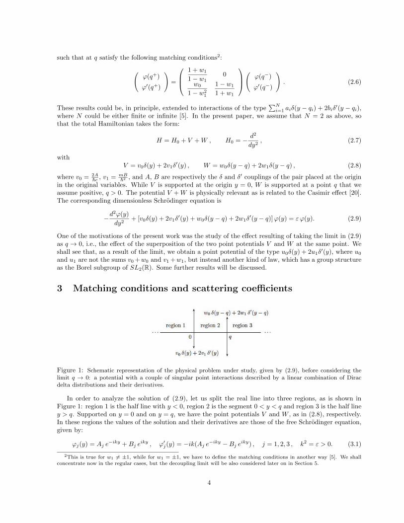
3 Matching conditions and scattering coefficients

Figure 1: Schematic representation of the physical problem under study, given by (2.9), before considering thelimit q → 0: a potential with a couple of singular point interactions described by a linear combination of Diracdelta distributions and their derivatives.

In order to analyze the solution of (2.9), let us split the real line into three regions, as is shown inFigure 1: region 1 is the half line with y < 0, region 2 is the segment 0 < y < q and region 3 is the half liney > q. Supported on y = 0 and on y = q, we have the point potentials V and W , as in (2.8), respectively.In these regions the values of the solution and their derivatives are those of the free Schrodinger equation,given by:

ϕj(y) = Aj e−iky +Bj e

iky , ϕ′j(y) = −ik(Aj e−iky −Bj eiky) , j = 1, 2, 3 , k2 = ε > 0. (3.1)

2This is true for w1 6= ±1, while for w1 = ±1, we have to define the matching conditions in another way [5]. We shallconcentrate now in the regular cases, but the decoupling limit will be also considered later on in Section 5.

4

Since the point potential V is defined by matching conditions like those in (2.6), we have that

(A2 +B2

−ik(A2 −B2)

)= Mv

(A1 +B1

−ik(A1 −B1)

), Mv =

1 + v1

1− v10

v0

1− v21

1− v1

1 + v1

. (3.2)

Defining the following matrix:

K =

(1 1−ik ik

), (3.3)

equation (3.2) becomes: (A2

B2

)= K−1MvK

(A1

B1

). (3.4)

This expression (3.4) gives the matching conditions at the point y = 0. At the point y = q the sameprocedure works after appropriate translation(

A3

B3

)= Q−1K−1MwKQ

(A2

B2

). (3.5)

and we finally obtain:(A3

B3

)= Q−1K−1MwKQK−1MvK

(A1

B1

)= Tq

(A1

B1

), (3.6)

where the definition of Tq is obvious, while Q and Mw are respectively:

Q =

(e−iqk 0

0 eiqk

), Mw =

1 + w1

1− w10

w0

1− w21

1− w1

1 + w1

. (3.7)

The Tq-matrix in (3.6) relates the asymptotic behaviour of the two linearly independent Jost scatteringsolutions at x << 0 with their counterparts at x >> 0, see e.g. [37]. The Tq-matrix elements satisfy theidentities:

detTq = T 11q T 22

q − T 12q T 12

q = 1 , T 11q = T 22

q , T 12q = T 21

q

such that Tq is in general an element of the group SL2(C). From the Tq-matrix one obtains the scatteringmatrix Sq by an standard procedure. Reshuffling the linear system (3.6) in the form(

A1

B3

)= Sq

(A3

B1

)(3.8)

one easily checks that

Sq =1

T 11q

(1 −T 12

q

T 21q detTq

), S†q =

1

T 11q

(1 T 21

q

−T 12q detTq

), S†qSq =

(1 00 1

), (3.9)

i.e., the scattering Sq-matrix arises as a 2 × 2 unitary matrix: S†qSq = SqS†q = 1. The transmission and

reflection coefficients provide the usual form of writing the Sq-matrix elements:

Sq =

(t(k) rR(k)rL(k) t(k)

). (3.10)

t(k) is the amplitude of the transmitted waves coming from the far left or from the far right. Time-reversalinvariant potentials give rise to identical transmission coefficients: tR(k; q) = tL(k; q) = t(k; q). However

5

the reflection amplitudes are different for incoming waves either from the far right or the far left such thatrR(k; q) 6= rL(k; q) because the potential is not parity invariant. Comparison of equations (3.9) and (3.10)shows that:

t(k; q) =1

T 11q (k)

, rR(k; q) = −T 12q (k)

T 11q (k)

, rL(k, q) =T 21q (k)

T 11q (k)

. (3.11)

Transmission and reflection coefficients were calculated in [20] when the two δ-δ′ point interactions weresymetrically located with respect to the origin. For the arrangement chosen in this paper we find fromformulas (3.11) :

rL(k; q) = −e−2iqk

(2k(v2

1 + 1)

+ iv0

)(4kw1 − iw0) + (4kv1 − iv0)

(2k(w2

1 + 1)− iw0

)∆(k)

, (3.12)

rR(k; q) =e2iqk

(2k(v2

1 + 1)− iv0

)(4kw1 + iw0) + (4kv1 + iv0)

(2k(w2

1 + 1)

+ iw0

)∆(k)

, (3.13)

t(k; q) =4k2(1− v2

1)(1− w21)

∆(k)(3.14)

∆(k) = e2ikq(v0 + 4ikv1)(w0 − 4ikw1) + (2kv21 + 2k + iv0)(2kw2

1 + 2k + iw0), (3.15)

where ∆(k) is a function of k and the other parameters of the problem.

3.1 Bound/antibound states and resonances

Complex zeroes of

T 11q (k) =

∆(k)

4k2(1− v21)(1− w2

1), (3.16)

which are poles of the Sq-matrix in the k-complex plane, give rise to bound or antibound states if arelocated on the purely imaginary, respectively positive or negative half-axis. Complex zeroes coming inpairs having opposite real part and identical imaginary part correspond to resonances.

The relevant physical information is encoded in the analysis of complex zeroes of T 11q (k), or equivalently

of ∆(k). In order to simplify this analysis, it is useful to make the following changes in the parameters in(3.16):

2kq = z, σ =qv0

1 + v21

, τ =qw0

1 + w21

, v =v1

1 + v21

, w =w1

1 + w21

. (3.17)

Then, ∆(k) = 0 is equivalent to

eiz = −(

z + iσ

σ + 2ivz

)(z + iτ

τ − 2iwz

), z = zr + izi, zr, zi ∈ R. (3.18)

Equation (3.18) can be considered as a complex or two-dimensional generalization of the so-called gener-alized Lambert equation (see [38, 39] and references quoted therein). From this complex Lambert equationwe can obtain two real equations, corresponding to the real and imaginary parts of (3.18):[

4vwz2r − (2vzi − σ)(2wzi + τ)

]cos zr − 2zr(τv + 4vwzi − σw) sin zr =

[(zi + σ)(zi + τ)− z2

r

]ezi . (3.19)

2zr(τv + 4vwzi − σw) cos zr +[4vwz2

r − (2vzi − σ)(2wzi + τ)]

sin zr = −zr(2zi + σ + τ)ezi . (3.20)

These expressions for real and imaginary parts of ∆(k) = 0 are rather complicated. A simpler compatibilitycondition is given by

e2zi =(4v2z2

r +(2vzi − σ)2

) (4w2z2

r + (2wzi + τ)2)

(z2r + (zi + σ)2) (z2

r + (zi + τ)2), (3.21)

which is, indeed, a generalization of the Lambert equation that includes two real variables. The solutionswe are looking for must satisfy (3.21), although (3.19)–(3.20) are more restrictive. First of all, we can

6

easily check that a simple solution of the system (3.19)–(3.20) is zr = 0, zi = 0, but this corresponds tok = 0, which is a pole of T 11

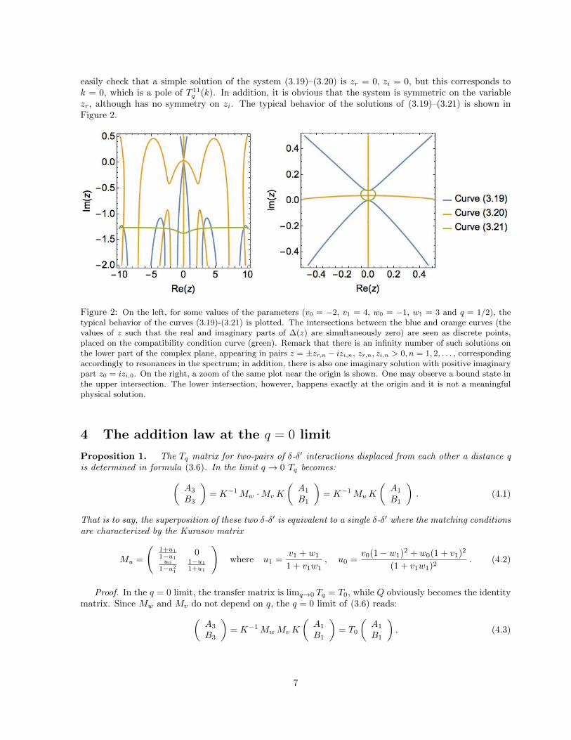
q (k). In addition, it is obvious that the system is symmetric on the variablezr, although has no symmetry on zi. The typical behavior of the solutions of (3.19)–(3.21) is shown inFigure 2.

Figure 2: On the left, for some values of the parameters (v0 = −2, v1 = 4, w0 = −1, w1 = 3 and q = 1/2), thetypical behavior of the curves (3.19)-(3.21) is plotted. The intersections between the blue and orange curves (thevalues of z such that the real and imaginary parts of ∆(z) are simultaneously zero) are seen as discrete points,placed on the compatibility condition curve (green). Remark that there is an infinity number of such solutions onthe lower part of the complex plane, appearing in pairs z = ±zr,n − izi,n, zr,n, zi,n > 0, n = 1, 2, . . . , correspondingaccordingly to resonances in the spectrum; in addition, there is also one imaginary solution with positive imaginarypart z0 = izi,0. On the right, a zoom of the same plot near the origin is shown. One may observe a bound state inthe upper intersection. The lower intersection, however, happens exactly at the origin and it is not a meaningfulphysical solution.

4 The addition law at the q = 0 limit

Proposition 1. The Tq matrix for two-pairs of δ-δ′ interactions displaced from each other a distance qis determined in formula (3.6). In the limit q → 0 Tq becomes:(

A3

B3

)= K−1Mw ·MvK

(A1

B1

)= K−1MuK

(A1

B1

). (4.1)

That is to say, the superposition of these two δ-δ′ is equivalent to a single δ-δ′ where the matching conditionsare characterized by the Kurasov matrix

Mu =

(1+u1

1−u10

u0

1−u21

1−u1

1+u1

)where u1 =

v1 + w1

1 + v1w1, u0 =

v0(1− w1)2 + w0(1 + v1)2

(1 + v1w1)2. (4.2)

Proof. In the q = 0 limit, the transfer matrix is limq→0 Tq = T0, while Q obviously becomes the identitymatrix. Since Mw and Mv do not depend on q, the q = 0 limit of (3.6) reads:(

A3

B3

)= K−1MwMvK

(A1

B1

)= T0

(A1

B1

). (4.3)

7

One may expect that the product of two Kurasov matrices MwMv is another Kurasov matrix. Thisassumption means that

MwMv =

1 + w1

1− w10

w0

1− w21

1− w1

1 + w1

1 + v1

1− v10

v0

1− v21

1− v1

1 + v1

=

1 + u1

1− u10

u0

1− u21

1− u1

1 + u1

= Mu. (4.4)

A lengthy but straightforward calculation shows that this is the case with the “composite”couplings:

u1 =v1 + w1

1 + v1w1, u0 =

v0(1− w1)2 + w0(1 + v1)2

(1 + v1w1)2, (4.5)

Thus, the collapsed two δ-δ′ pairs are tantamount to a single point potential of the form u0δ(y) + 2u1δ′(y)

defined by the transfer matrix T0 = K−1MuK, q. e. d.One would have expected another result such as an additive rule of the type u0 = v0 + w0 and u1 =

v1 + w1, due to the form of point potentials that converge. In fact for zero δ′ couplings we would obtain:(1 0

w0 1

)(1 0

v0 1

)=

(1 0

w0 + v0 1

)and the fusion of two δ point potentials is a pure abelian process. Nonetheless, the addition law (4.5) isquite interesting. First of all, the first equation in (4.5) resembles the addition law of velocities in specialrelativity. However, the second one looks more complicated. In any case, one natural question we maypose is if the composition law (4.5) has a structure of a group and, if this is the case, which group this canbe.

Checking the group structure is quite simple. The product of two matrices Mv and Mw as in (4.4)gives another matrix with identical structure. This gives the product law. The associativity comes fromthe associativity of the product of matrices. The identity of the group is the 2× 2 identity matrix I, whichcorresponds to take both parameters equal to zero in (2.6), M0 = I. The inverse of Mv is a matrix Ms sothat MvMs = I. The calculation is straightforward. For Mv as defined in (3.2) one finds

Ms =

1− v1

1 + v10

−v0

1− v21

1 + v1

1− v1

, (4.6)

which shows that taking the inverse in our group of matrices is equivalent to the transformation (v0, v1)→(−v0,−v1). We may denote the inverse of Mv as M−v. Thus, the structure of group in our set of matriceshas been confirmed. Furthermore, there are two other remarkable properties of matrices in this group:

(i) Non commutativity:

MvMw −MwMv =

0 0

4(v0w1 − w0v1)

(1− v21)(1− w2

1)0

. (4.7)

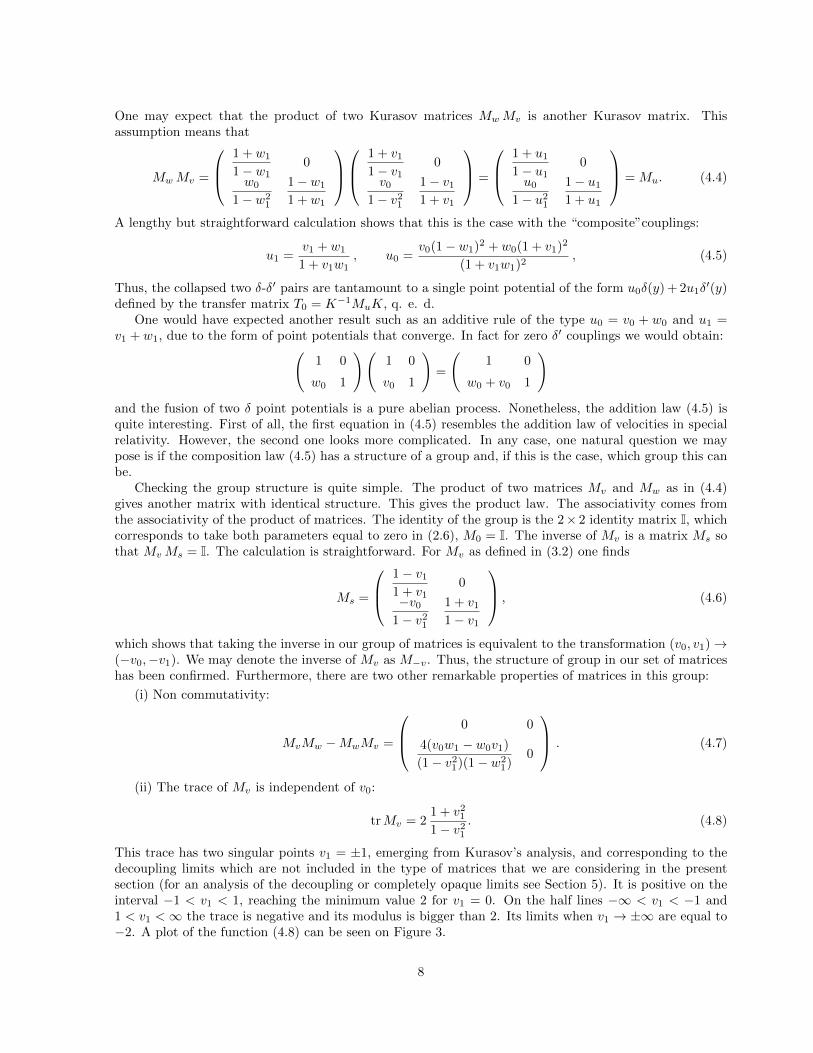
(ii) The trace of Mv is independent of v0:

trMv = 21 + v2

1

1− v21

. (4.8)

This trace has two singular points v1 = ±1, emerging from Kurasov’s analysis, and corresponding to thedecoupling limits which are not included in the type of matrices that we are considering in the presentsection (for an analysis of the decoupling or completely opaque limits see Section 5). It is positive on theinterval −1 < v1 < 1, reaching the minimum value 2 for v1 = 0. On the half lines −∞ < v1 < −1 and1 < v1 <∞ the trace is negative and its modulus is bigger than 2. Its limits when v1 → ±∞ are equal to−2. A plot of the function (4.8) can be seen on Figure 3.

8

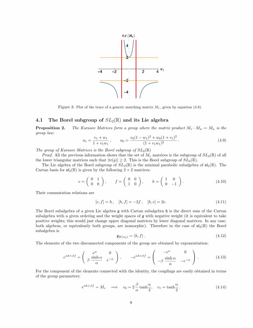
Figure 3: Plot of the trace of a generic matching matrix Mv, given by equation (4.8).

4.1 The Borel subgroup of SL2(R) and its Lie algebra

Proposition 2. The Kurasov Matrices form a group where the matrix product Mv ·Mw = Mu is thegroup law:

u1 =v1 + w1

1 + v1w1, u0 =

v0(1− w1)2 + w0(1 + v1)2

(1 + v1w1)2. (4.9)

The group of Kurasov Matrices is the Borel subgroup of SL2(R)Proof. All the previous information shows that the set of Mv matrices is the subgroup of SL2(R) of all

the lower triangular matrices such that |tr(g)| ≥ 2. This is the Borel subgroup of SL2(R).The Lie algebra of the Borel subgroup of SL2(R) is the minimal parabolic subalgebra of sl2(R). The

Cartan basis for sl2(R) is given by the following 2× 2 matrices:

e =

(0 10 0

), f =

(0 01 0

), h =

(1 00 −1

). (4.10)

Their commutation relations are

[e, f ] = h , [h, f ] = −2f , [h, e] = 2e. (4.11)

The Borel subalgebra of a given Lie algebra g with Cartan subalgebra h is the direct sum of the Cartansubalgebra with a given ordering and the weight spaces of g with negative weight (it is equivalent to takepositive weights; this would just change upper diagonal matrices by lower diagonal matrices. In any case,both algebras, or equivalently both groups, are isomorphic). Therefore in the case of sl2(R) the Borelsubalgebra is

gK(x0) = 〈h, f〉 . (4.12)

The elements of the two disconnected components of the group are obtained by exponentiation:

eαh+βf =

(eα 0

βsinhα

αe−α

), −eαh+βf =

−eα 0

−β sinhα

α−e−α

. (4.13)

For the component of the elements connected with the identity, the couplings are easily obtained in termsof the group parameters:

eαh+βf = Mv =⇒ v0 = 2β

αtanh

α

2, v1 = tanh

α

2. (4.14)

9

On the other hand, for the elements in the other connected component, we have:

−eαh+βf = Mv =⇒ v0 = 2β

αcoth

α

2, v1 = coth

α

2. (4.15)

The composition law of the group can be expressed in terms of these exponentials. In fact,

eα1h+β1f eα2h+β2f = eαh+βf (4.16)

with

α = α1 + α2 , β =(α1 + α2) (eα2α2β1 sinh (α1) + e−α1α1β2 sinh (α2))

α1α2 sinh(α1 + α2). (4.17)

This concludes the discussion on the group structure. Q. E. D

4.2 Reflection and transmission coefficients due to a single δ-δ′ interaction atthe origin

Proposition 3. The q = 0 limit of the scattering coefficients of two a priori separated pairs of δ-δ′

interactions exactly coincide with the scattering coefficients produced by a single δ-δ′ pair with couplingsdetermined from the Mu = Mv ·Mw Kurasov matrix. In terms of the scattering matrix we can write:

limq→0

Sq(Mv,Mw) = S(Mv ·Mw) = S(Mu). (4.18)

Hence the scattering matrices produced by two superimposed pairs of δ-δ′ interactions give rise to a repre-sentation of the non-abelian composition law of Kurasov matrices.

Proof. The linear map between asymptotic scattering Jost solutions respectively in the far right andthe far left, (

A2

B2

)= Z

(A1

B1

),

produced by a single point interaction V (x) = u0δ(x) + 2u1δ′(x) is provided by a similarity transformation

of the Kurasov matrix :

Z = K−1MuK , Mu =

1 + u1

1− u10

u0

1− u21

1− u1

1 + u1

.

We obtain for the Z-matrix elements

Z11(k) =2k(1 + u2

1) + iu0

2k(1− u21)

= Z22(k) , Z12(k) =4ku1 + iu0

2k(1− u21)

= Z21, (4.19)

where the bar stands for complex conjugation. From this information one reads the scattering coefficients

rR(k) = −Z12(k)

Z11(k)= − 4ku1 + iu0

2k(u1 + 1) + iu0, rL(k) =

Z21(k)

Z11(k)=

4ku1 − iu0

2k(u21 + 1) + iu0

, (4.20)

t(k) =1

Z11(k)= − 2k(u2

1 − 1)

2k(u21 + 1) + iu0

, (4.21)

in perfect agreement with the results in [12].Finally, we compare these scattering coefficients with those obtained from the T0-matrix that describe

the map between asymptotic Jost solutions when the distance q from one δ-δ′ point interaction to the other

10

tends to zero. The outcome is:

rL(k; 0) = −T120 (k)

T 110 (k)

= −v1 ((v1 + 2)w0 + 4ik) + 4ikv1w1 (v1 + w1) + 4ikw1 + v0 (w1 − 1) 2 + w0

−2ikw1 ((v21 + 1)w1 + 4v1)− 2ik (v2

1 + 1) + (v1 + 1) 2w0 + v0 (w1 − 1) 2, (4.22)

rR(k; 0) =T 21

0 (k)

T 110 (k)

=v1 (− (v1 + 2)w0 + 4ik) + 4ikv1w1 (v1 + w1) + 4ikw1 − v0 (w1 − 1) 2 − w0

−2ikw1 ((v21 + 1)w1 + 4v1)− 2ik (v2

1 + 1) + (v1 + 1) 2w0 + v0 (w1 − 1) 2, (4.23)

t(k; 0) =1

T 110 (k)

=2k(v2

1 − 1) (w2

1 − 1)

2kw1 ((v21 + 1)w1 + 4v1) + 2k (v2

1 + 1) + i (v1 + 1) 2w0 + iv0 (w1 − 1) 2, (4.24)

to check that the addition law

u1 =v1 + w1

1 + v1w1, u0 =

v0(1− w1)2 + w0(1 + v1)2

(1 + v1w1)2,

also works for the scattering coefficients, q.e.d.

5 The left-right decoupling values of the δ′ couplings

We have seen that there are singularities of the Kurasov matrix at the critical points, v1 = ±1 andw1 = ±1. One may expect that these critical cases where the transmission coefficients are zero do notcontribute to the group structure that we have previously analyzed. The completely opaque potentials asgiven in equations (2.8) have clearly one of the following four forms:

V = v0δ(x)± 2δ′(x) and/or W = w0δ(x− q)± 2δ′(x− q) . (5.1)

In order to define these potentials, we obviously cannot use matching conditions of the form (2.6) that aresingular. Instead, we shall impose [5]:

1. For v1 = 1:

ϕ(0−) = 0 , ϕ′(0+) =v0

4ϕ(0+). (5.2)

2. For w1 = 1:

ϕ(q−) = 0 , ϕ′(q+) =w0

4ϕ(q+) . (5.3)

Thus, we set Dirichlet boundary conditions on the left of the two points x = 0 and x = q, whereasRobin boundary conditions are chosen on the right hand side of x = 0 and x = q, see [20]. In thetwo remaining cases the matching conditions are the mirror images of the previous ones.

3. For v1 = −1:

ϕ(0+) = 0 , ϕ′(0−) = −v0

4ϕ(0−). (5.4)

4. For w1 = −1:

ϕ(q+) = 0 , ϕ′(q−) = −w0

4ϕ(q−) . (5.5)

We remain, however, in the physical situation depicted in Figure 1, were the plane waves and their deriva-tives are written as in (3.1). There are eight possible configurations involving at least one decouplingconfiguration of the couplings: either the two δ-δ′ interactions build opaque walls both at x = 0 and x = q,or, there is no transmission only at one point. We discuss first the cases when the two δ′ couplings takethe decoupling limit.

11

5.1 Two δ′ couplings in the decoupling limit

There are four cases in which we have decoupling situations both at x = 0 and x = q. Let us considerthem separately.

Case 1: v1 = 1, w1 = 1.The boundary conditions are given by (5.2) and (5.3). Let us consider the situation on the interval [0, q].For x = 0, ϕ′(0+) = v0

4 ϕ(0+) is written as:

−ik(A2 −B2) =v0

4(A2 +B2) =⇒ A2

B2= −v0 − 4ik

v0 + 4ik= − exp

(−2i arctan

4k

v0

). (5.6)

For x = q, we write ϕ(q−) = 0 as

A2 e−ikq +B2 e

ikq = 0 =⇒ A2

B2= −e2ikq . (5.7)

Then, we have a transcendental equation, which can be written either in the form of a generalized Lambertequation:

e2ikq =v0 − 4ik

v0 + 4ik, (5.8)

or in terms of the function arctan as

kq = − arctan4k

v0=⇒ tan(kq) = −4k

v0. (5.9)

This transcendental equation has a countably infinite number of solutions, kn, that give the energy levelscorresponding to this situation. In the limit q = 0, we have only one solution, k = 0. Outside the interval[0, q], we have the equations

ϕ(0−) = 0 =⇒ A1 +B1 = 0; ϕ′(q+) =w0

4ϕ(q+) =⇒ A3

B3= −e2ikq w0 − 4ik

w0 + 4ik. (5.10)

These are relations between coefficients, which do not provide of any further information, so that we shallnot refer for similar situations which will appear for all other cases.

Case 2: v1 = 1, w1 = −1.The boundary conditions are (5.2) for x = 0 and (5.5) for x = q. The condition at x = 0 has already beenstudied, providing equation (5.6), so that let us consider the new boundary condition at x = q. It comesfrom ϕ′(q−) = −w0

4 ϕ(q−):

A2

B2= −e2ikq w0 + 4ik

w0 − 4ik= −e2ikq exp

(2i arctan

4k

w0

). (5.11)

This equation is to be compared to (5.6). The result given in terms of a generalized Lambert equation is:

e2ikq =v0 − 4ik

v0 + 4ik

w0 − 4ik

w0 + 4ik. (5.12)

This transcendental equation can be written in another way by playing with the formulas for the arctan.Note that from (5.12) we obtain straightforwardly the following expression:

−kq = arctan4k

w0+ arctan

4k

v0=⇒ tan(kq) = − 4k(w0 + v0)

w0v0 − 16k2. (5.13)

This new transcendental equation gives another set of energy eigenvalues (see Figure 4 right). In the limitq = 0, we have only one solution: k = 0.

12

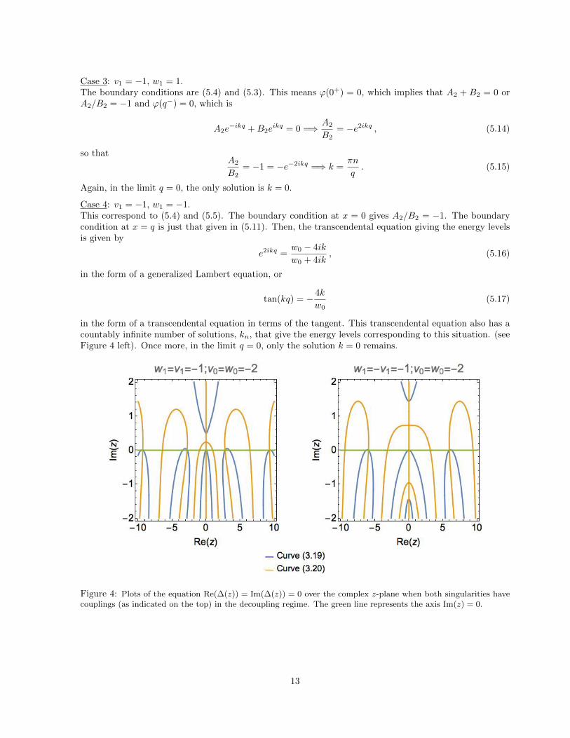
Case 3: v1 = −1, w1 = 1.The boundary conditions are (5.4) and (5.3). This means ϕ(0+) = 0, which implies that A2 + B2 = 0 orA2/B2 = −1 and ϕ(q−) = 0, which is

A2e−ikq +B2e

ikq = 0 =⇒ A2

B2= −e2ikq , (5.14)

so thatA2

B2= −1 = −e−2ikq =⇒ k =

πn

q. (5.15)

Again, in the limit q = 0, the only solution is k = 0.

Case 4: v1 = −1, w1 = −1.This correspond to (5.4) and (5.5). The boundary condition at x = 0 gives A2/B2 = −1. The boundarycondition at x = q is just that given in (5.11). Then, the transcendental equation giving the energy levelsis given by

e2ikq =w0 − 4ik

w0 + 4ik, (5.16)

in the form of a generalized Lambert equation, or

tan(kq) = − 4k

w0(5.17)

in the form of a transcendental equation in terms of the tangent. This transcendental equation also has acountably infinite number of solutions, kn, that give the energy levels corresponding to this situation. (seeFigure 4 left). Once more, in the limit q = 0, only the solution k = 0 remains.

Figure 4: Plots of the equation Re(∆(z)) = Im(∆(z)) = 0 over the complex z-plane when both singularities havecouplings (as indicated on the top) in the decoupling regime. The green line represents the axis Im(z) = 0.

13

5.2 Only one δ′ coupling in the decoupling limit

Let us consider now the four cases in which we have a decoupling and a regular coupling.

Case 1: v1 = 1, w1 6= ±1.From v1 = 1, that is, from (5.2), we know that the conditions A1 = −B1 6= 0 and (5.6) must be satisfied,that is

ϕ1(y) ∝ sin(ky), A2 = −v0 − 4ik

v0 + 4ikB2. (5.18)

Note that the system behaves as if there is an impenetrable barrier at x = 0. The coefficients A3, B3 areobtained from A2, B2 as in (3.5)

(A3

B3

)=

2k(1 + w2

1) + iw0

2k(1− w21)

e2ikq 4kw1 + iw0

2k(1− w21)

e−2ikq 4kw1 − iw0

2k(1− w21)

2k(1 + w21)− iw0

2k(1− w21)

(A2

B2

). (5.19)

All the relevant information about bound states, antibound states and resonances is obtained imposing theso-called purely outgoing boundary condition, which in our case is A3 = 0. Using (5.18) and (5.19) we get

e2ikq =v0 − 4ik

v0 + 4ik

2k(1 + w21) + iw0

4kw1 + iw0. (5.20)

This equation is the equivalent of ∆(k) = 0, where ∆(k) is given in (3.15), which provides the relevantinformation in the non-decoupling case. Indeed, (5.20) is obtained making v1 = 1 in ∆(k) = 0. Theanalysis in this case is similar to the one carried out previously in Section 3.1.

We are interested especially in the case where q → 0. Then, from (5.20) we get

(v0 + 4ik)(4kw1 + iw0) = (v0 − 4ik)(2k(1 + w21) + iw0). (5.21)

The complex solutions of this equation are the following:

k0 = 0, k1 = −i 4w0 + v0(1− w1)2

4(1 + w1)2. (5.22)

The solution k = 0 is not relevant, but the other produces interesting results: If 4w0 + v0(1−w1)2 < 0, k1

is on the positive imaginary axis and it corresponds to a bound state, and if 4w0 +v0(1−w1)2 > 0, k1 is onthe negative imaginary axis and it corresponds to an anti-bound state. The curves solving the equationsRe(∆) = Im(∆) = 0 for this case are represented in Figure 5 left

Case 2: v1 = −1, w1 6= ±1.The system behaves also as if there were an impenetrable barrier at x = 0. Now, from v1 = −1 (orequivalently from (5.4)), we find the condition A2/B2 = −1 and consequently (5.19), which must be alsosatisfied. Then, the purely outgoing boundary condition A3 = 0 implies that (see Figure 5 right)

e2ikq =2k(1 + w2

1) + iw0

4kw1 + iw0. (5.23)

In the limit q → 0 we get the condition k(1− w1)2 = 0, which has the unique solution k = 0.

Case 3: v1 6= ±1, w1 = 1.In this situation we must take into account (5.3) and (3.4). The first pair of equations shows the presenceof a kind of impenetrable barrier, now in x = q, and also the fact that A2 = −e2ikqB2. Equation (3.4) canbe rewritten in the form

(A1

B1

)= K−1M−1

v K

(A2

B2

)=

2k(1 + v2

1)− iv0

2k(1− v21)

−4kv1 + iv0

2k(1− v21)

−4kv1 + iv0

2k(1− v21)

2k(1 + v21) + iv0

2k(1− v21)

(A2

B2

). (5.24)

14

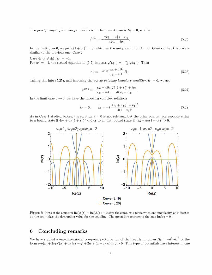
The purely outgoing boundary condition is in the present case is B1 = 0, so that

e2ikq = −2k(1 + v21) + iv0

4kv1 − iv0. (5.25)

In the limit q → 0, we get k(1 + v1)2 = 0, which as the unique solution k = 0. Observe that this case issimilar to the previous one, Case 2.

Case 4: v1 6= ±1, w1 = −1.For w1 = −1, the second equation in (5.5) imposes ϕ′(q−) = −w0

4 ϕ(q−). Then

A2 = −e2ikq w0 + 4ik

w0 − 4ikB2. (5.26)

Taking this into (5.25), and imposing the purely outgoing boundary condition B1 = 0, we get

e2ikq = −w0 − 4ik

w0 + 4ik

2k(1 + v21) + iv0

4kv1 − iv0. (5.27)

In the limit case q → 0, we have the following complex solutions

k0 = 0, k1 = −i 4v0 + w0(1 + v1)2

4(1− v1)2. (5.28)

As in Case 1 studied before, the solution k = 0 is not relevant, but the other one, k1, corresponds eitherto a bound state if 4v0 + w0(1 + v1)2 < 0 or to an anti-bound state if 4v0 + w0(1 + v1)2 > 0.

Figure 5: Plots of the equation Re(∆(z) = Im(∆(z) = 0 over the complex z-plane when one singularity, as indicatedon the top, takes the decoupling value for the coupling. The green line represents the axis Im(z) = 0.

6 Concluding remarks

We have studied a one-dimensional two-point perturbation of the free Hamiltonian H0 = −d2/dx2 of theform v0δ(x) + 2v1δ

′(x) +w0δ(x− q) + 2w1δ′(x− q) with q > 0. This type of potentials have interest in one

15

dimensional quantum field theory and on the study of the Casimir effect as shown by previous work of ourgroup [23, 22, 20]. We have obtained two remarkable unexpected results.

The former refers to the limit q → 0. The result is a point potential of the form u0δ(x) + 2u1δ′(x),

where u0 and u1 are not the sums v0 +w0 and v1 +w1 respectively, but more complicated functions of thesearguments instead. A law of composition for the coefficients of the deltas is produced with structure ofgroup which coincides with the Borel subgroup of SL2(R). From the analysis of reflection and transmissioncoefficients, we obtain the same group law.

The second one comes from the analysis of the decoupling cases which arises by the choices v1 = ±1(decoupling case at x = 0) and w1 = ±1 (decoupling case at x = q). When considering the decoupling casesat x = 0 and x = q, the barrier seems to be impenetrable at these points so that no scattering states areproduced. One finds bound or antibound states as solutions of a generalized Lambert equation on termsof the momentum. When the decoupling regime is produced at one point only (either x = 0 or x = q), wehave impenetrability at this point and scattering through the other one and resonances (as pair of polesof the analytic continuation of the S-matrix in the momentum representation) can be found. However, itis quite remarkable to note that these poles may lie on the real axis if at least one of the δ′ couplings iscomplex. This situation may violate a widely accepted causality condition [40].

Finally, we mention that in the course of this paper we have clarified the relation between two apparentlydifferent ways of characterizing self-adjoint extensions of the H0 operator. The first one is based on thematching conditions determined from the Kurasov matrices. We have shown that they form the Borelsubgroup of SL2(R). The standard approach to deal with self-adjoint extensions of symmetric operators,coming back to von Neumann, is through unitary matrices, see e.g. the previous works [7, 8, 9] by Asorey,Munoz-Castaneda et al. The connection from these two points of view starts from the isomorphism betweenthe SL2(R) and SU1,1(C) groups. In fact they are conjugate subgroups inside GL2(R):

g SL2(R) g−1 = SU1,1(R) , g =

(1 −i1 i

).

The matching conditions (2.6) become in the SU1,1(C) framework:(ϕ(q+)− iϕ′(q+)ϕ(q+) + iϕ′(q+)

)= Wv

(ϕ(q−)− iϕ′(q−)ϕ(q−) + iϕ′(q−)

), (6.1)

where the Wv is conjugated to the Kurasov matrix Mv through the action of g:

Wv = gMv g−1 =

1

2(1− v21)

(2(1 + v2

1)− iv0 4v1 − iv0

4v1 + iv0 2(1 + v21) + iv0

). (6.2)

In a parallel reshufling of the linear system (6.1) to that performed to define the Sq scattering matrix fromthe Tq matrix and passing from the (3.6) equation to (3.8) and (3.9) we rewrite (6.1) in the form(

ϕ(q−)− iϕ′(q−)ϕ(q+) + iϕ′(q+)

)= Uv

(ϕ(q+)− iϕ′(q+)ϕ(q−) + iϕ′(q−)

), (6.3)

where the unitary matrix Uv is obtained from Wv and reads

Uv =1

W 11v

(1 −W 12

v

W 21v detWv

)=

2(1− v21)

2(1 + v21)− iv0

(1 −4v1+iv0

2(1−v21)4v1+iv02(1−v21)

1

). (6.4)

In this indirect way the Kurasov matrices determining the matching conditions that define the δ-δ′ in-teractions are related to a subset of the U(2) group which in turn characterizes a variety of self-adjointextensions of the H0 operator in the standard manner.

A remarkable fact is the following: even though Mv and Wv are singular matrices at the decouplinglimit v1 = ±1 the corresponding unitary matrices are regular:

Uv

∣∣∣v1=1

=

(0 −1

4+iv04−iv0 0

), Uv

∣∣∣v1=−1

=

(0 4+iv0

4−iv0−1 0

). (6.5)

16

Writing the linear system (6.4) for the decoupling limit of the coupling v1 = 1 we obtain two equations.First,

−(ϕ(q−) + iϕ′(q−)) = ϕ(q−)− iϕ′(q−) ⇒ ϕ(q−) = 0 , (6.6)

i.e., Dirichlet boundary conditions are satisfied reaching the point q from the left. Second,

4 + iv0

4− iv0(ϕ(q+)− iϕ′(q+)) = ϕ(q+) + iϕ′(q+) ⇒ ϕ(q+)− 4

v0ϕ′(q+) = 0 (6.7)

sets Robin boundary conditions at q coming from the right. If the other decoupling value for the coupling,v1 = −1, is chosen the situation is identical but the conditions at q from the left or from the right areexchanged. The results above is in perfect agreement with the Kurasov matching conditions at decouplinglimit of the couplings, as expressed in formula (5.2). Finally, we mention that in the usual treatment thissituation is determined from diagonal rather than anti-diagonal matrices. To meet this criterion one merelymultiply (6.5) by the σ1 Pauli matrix.

Finally, we extract some physical consequences from the non-abelian superposition law for the δ-δ′

potentials:

1. The quantum self-energy of two δ-δ′ configurations due to quantum vacuum scalar fluctuations shouldinherit somehow some features from the non-abelian composition law. A wel known procedureto regularize such divergent quantity is to start from the heat trace of the Hamiltonian operator:hH(t) = TrL2exp[−tH], where t is Schwinger proper time. This spectral function is obtained for anySchrodinger Hamiltonian in terms of the bound state energies and the spectral density, defined inturn from the total phase shift, see the two formulas just above (32) in [22]. From the total phaseshift produced by the δ-δ′ potential determined by the Mv Kurasov matrix and the bound stateenergy we find:

hH (t; Mv) = etv2

04(v2

1+1)2

(2iπ erfc

( √tv0

2 (v21 + 1)

)+ θ (−v0)− 4iπ

), (6.8)

where erfc is the complementary error function and θ the Heaviside step function. It is of note that theexact heat kernel for a single δ-δ′ is well defined in the decoupling limit v1 → ±1. We conjecture thattaking the zero distance limit in the double δ-δ′ potential, the heat trace for the superposed potentialwill be of the form hH (t; Mv ·Mw) = hH (t; Mu). The quantum vacuum energy is essentially thespectral zeta function evaluated at s = −1/2. This second spectral function is obtained from theheat trace via Mellin’s transform of the heat trace: ζH(s) = 1

Γ(s)

∫∞0dt ts−1hH(t), where Γ(s) is

Euler Gamma function and s a complex parameter. s = −1/2 is a pole of the meromorphic functionζH(s) in C. One regularizes the divergent quantum vacuum energy by assigning to ζH its value ina regular point. What the non-abelian addition law tell us are the values of the parameters u0 andu1 as functions of v0, w0, v1, w1 entering in this regularized expression after the q = 0 limit has beentaken.

2. An ideal model of electric conductivity in solids is provided by a δ-Dirac comb where δ-point interac-tions sit at the ions sites. This model can be enriched in a twofold way: (1) δ′ potentials are addedat every site of the lattice. (2) Two species of ions, henceforth two species of δ-δ′ interactions, suchthat the solid is characterized by the periodic potential

V (x) =∑n∈Z

(v0δ(x− nq) + v1δ(x− nq) + u0δ(x− nq + p) + u1δ(x− nq + p)) (6.9)

are considered. There are two limits to a single species: p → 0, q. Unlike in the Dirac comb of twospecies where the two limits are equivalent, the two merging processes are different in the (6.9) combdue to the non-abelian superposition law. In fact, allowing p to vary we have an infinitely repeatedCasimir piston, which can be reduced to one piston by restricting the system to the primitive cell.

17

Acknowledgements

We acknowledge the financial support of the Spanish MINECO (Project MTM2014-57129-C2-1-P) andJunta de Castilla y Leon (UIC 011). JMMC would like to acknowledge the fruitful discussions withMichael Bordag, Klaus Kirsten and Manuel Asorey.

References

[1] S. Albeverio, F. Gesztesy, R. Høegh-Krohn, and H. Holden. Solvable models in quantum mechanics.AMS Chelsea Publishing, Providence, RI, second edition, 2005.

[2] A V Zolotaryuk and Yaroslav Zolotaryuk. A zero-thickness limit of multilayer structures: a resonant-tunnelling δ′-potential. Journal of Physics A: Mathematical and Theoretical, 48(3):035302, 2015.

[3] A.V. Zolotaryuk and Yaroslav Zolotaryuk. Controllable resonant tunnelling through single-point po-tentials: A point triode. Physics Letters A, 379(6):511 – 517, 2015.

[4] M Gadella, F J H Heras, J Negro, and L M Nieto. A delta well with a mass jump. Journal of PhysicsA: Mathematical and Theoretical, 42(46):465207, 2009.

[5] P. Kurasov. Distribution theory for discontinuous test functions and differential operators with gen-eralized coefficients. Journal of Mathematical Analysis and Applications, 201(1):297 – 323, 1996.

[6] Sergio Albeverio and Pavel Kurasov. Singular Perturbations of Differential Operators, volume 271 ofLondon Mathematical Society: Lecture Notes Series. Cambridge University Press, 2000.

[7] M. Asorey, D. Garcia-Alvarez, and J.M. Munoz-Castaneda. Casimir Effect and Global Theory ofBoundary Conditions. Journal of Physics A: Mathematical and Theoretical, 39:6127–6136, 2006.

[8] M. Asorey and J.M. Munoz-Castaneda. Attractive and Repulsive Casimir Vacuum Energy with Gen-eral Boundary Conditions. Nucl. Phys., B874:852–876, 2013.

[9] J.M. Munoz-Castaneda, Klaus Kirsten, and M. Bordag. QFT over the finite line. Heat kernel coeffi-cients, spectral zeta functions and selfadjoint extensions. Lett. Math. Phys., 105(4):523–549, 2015.

[10] Yuriy Golovaty. Schrodinger operators with (alpha delta’+ beta delta)-like potentials: norm resolventconvergence and solvable models. Methods Funct. Anal. Topology, 18(3):243–255, 2012.

[11] Marcos Calcada, Jose Tadeu Lunardi, Luiz A. Manzoni, and Wagner Monteiro. Distributional ap-proach to point interactions in one-dimensional quantum mechanics. Frontiers in Physics, 2(23),2014.

[12] M. Gadella, J. Negro, and L.M. Nieto. Bound states and scattering coefficients of the −aδ(x) + bδ′(x)potential. Physics Letters A, 373(15):1310 – 1313, 2009.

[13] P. Seba. Some remarks on the δ′-interaction in one dimension. Reports on Mathematical Physics,24(1):111 – 120, 1986.

[14] Sergio Albeverio, Silvestro Fassari, and Fabio Rinaldi. A remarkable spectral feature of the schrodingerhamiltonian of the harmonic oscillator perturbed by an attractive δ′-interaction centred at the ori-gin: double degeneracy and level crossing. Journal of Physics A: Mathematical and Theoretical,46(38):385305, 2013.

[15] A. V. Zolotaryuk. Boundary conditions for the states with resonant tunnelling across the δ′-potential.Phys. Lett. A, 374:1636–1641, April 2010.

18

[16] A V Zolotaryuk and Y Zolotaryuk. Controlling a resonant transmission across the δ′-potential: theinverse problem. Journal of Physics A: Mathematical and Theoretical, 44(37):375305, 2011.

[17] A V Zolotaryuk and Y Zolotaryuk. Corrigendum: Controlling a resonant transmission across the δ′-potential: the inverse problem. Journal of Physics A: Mathematical and Theoretical, 45(11):119501,2012.

[18] Sergio Albeverio, Silvestro Fassari, and Fabio Rinaldi. The discrete spectrum of the spinless one-dimensional salpeter hamiltonian perturbed by δ-interactions. Journal of Physics A: Mathematicaland Theoretical, 48(18):185301, 2015.

[19] V.L. Kulinskii and D. Yu. Panchenko. Physical structure of point-like interactions for one-dimensionalschrdinger operator and the gauge symmetry. Physica B: Condensed Matter, 472:78 – 83, 2015.

[20] J.M. Munoz Castaneda and J. Mateos Guilarte. δ − δ′ generalized Robin boundary conditions andquantum vacuum fluctuations. Phys. Rev., D91(2):025028, 2015.

[21] J.J. Alvarez, M. Gadella, L.P. Lara, and F.H. Maldonado-Villamizar. Unstable quantum oscillatorwith point interactions: Maverick resonances, antibound states and other surprises. Physics LettersA, 377(38):2510 – 2519, 2013.

[22] Jose M. Munoz-Castaneda, J. Mateos Guilarte, and A. Moreno Mosquera. Quantum vacuum energiesand Casimir forces between partially transparent δ-function plates. Phys. Rev., D87:105020, 2013.

[23] J. Mateos Guilarte and Jose M. Munoz-Castaneda. Double-delta potentials: one dimensional scatter-ing. The Casimir effect and kink fluctuations. Int. J. Theor. Phys., 50:2227–2241, 2011.

[24] M. Bordag and J.M. Munoz-Castaneda. Quantum vacuum interaction between two sine-Gordon kinks.Journal of Physics A: Mathematical and Theoretical., 45:374012, 2012.

[25] Michael Bordag. Vacuum energy in smooth background fields. Journal of Physics A: Mathematicaland Theoretical, 28:755–766, 1995.

[26] G Barton. Casimir energies of spherical plasma shells. Journal of Physics A: Mathematical andGeneral, 37(3):1011, 2004.

[27] M. Bordag. Monoatomically thin polarizable sheets. Phys. Rev. D, 89:125015, Jun 2014.

[28] A. Zee. Quantum Field Theory in a Nutshell: (Second Edition). In a Nutshell series. PrincetonUniversity Press, 2010.

[29] Guglielmo Fucci, Klaus Kirsten, and Pedro Morales. Pistons Modelled by Potentials. Springer Proc.Phys., 137:313–322, 2011.

[30] Guglielmo Fucci and Klaus Kirsten. Conical Casimir Pistons with Hybrid Boundary Conditions.Journal of Physics A: Mathematical and Theoretical, 44:295403, 2011.

[31] Guglielmo Fucci and Klaus Kirsten. The Casimir Effect for Generalized Piston Geometries. Int. J.Mod. Phys. Conf. Ser., 14:100–114, 2012.

[32] Guglielmo Fucci. Casimir Pistons with General Boundary Conditions. Nucl. Phys., B891:676–699,2015.

[33] Leon N. Cooper. Bound electron pairs in a degenerate fermi gas. Phys. Rev., 104:1189–1190, 1956.

[34] C. J. Pethick and Henrik Smith. Bose-Einstein condensation in dilute gases. Cambridge UniversityPress, second ed. edition, 2008.

19

[35] I. E. Antoniou, M. Gadella, E. Hernandez, A. Jauregui, Y. Melnikov, A. Mondragon, and G. P. Pronko.Gamow vectors for barrier wells. Chaos Solitons and Fractals, 12:2719–2736, 2001.

[36] Juan Luis Garcia-Pomar, Alexey Yu. Nikitin, and Luis Martin-Moreno. Scattering of graphene plas-mons by defects in the graphene sheet. ACS Nano, 7(6):4988–4994, 2013.

[37] L. J. Boya. Quantum mechanical scattering in one dimension. Nuovo Cimento Rivista Serie,31(2):020000–139, February 2008.

[38] Tony C Scott, Monique Aubert-Frecon, and Johannes Grotendorst. New approach for the electronicenergies of the hydrogen molecular ion. Chem. Phys., 324(2):323–338, 2006.

[39] Tony C. Scott, Robert Mann, and Roberto E. Martinez II. General Relativity and Quantum Mechan-ics: towards a Generalization of the Lambert W Function. Appl. Algebra Eng., Commun. Comput.,17(1):41–47, 2006.

[40] H. M. Nussenzveig. Causality and dispersion relations. Academic Press New York, 1972.

20