Logic Programming

CS 6371: Advanced Programming Languages

FP vs. LP

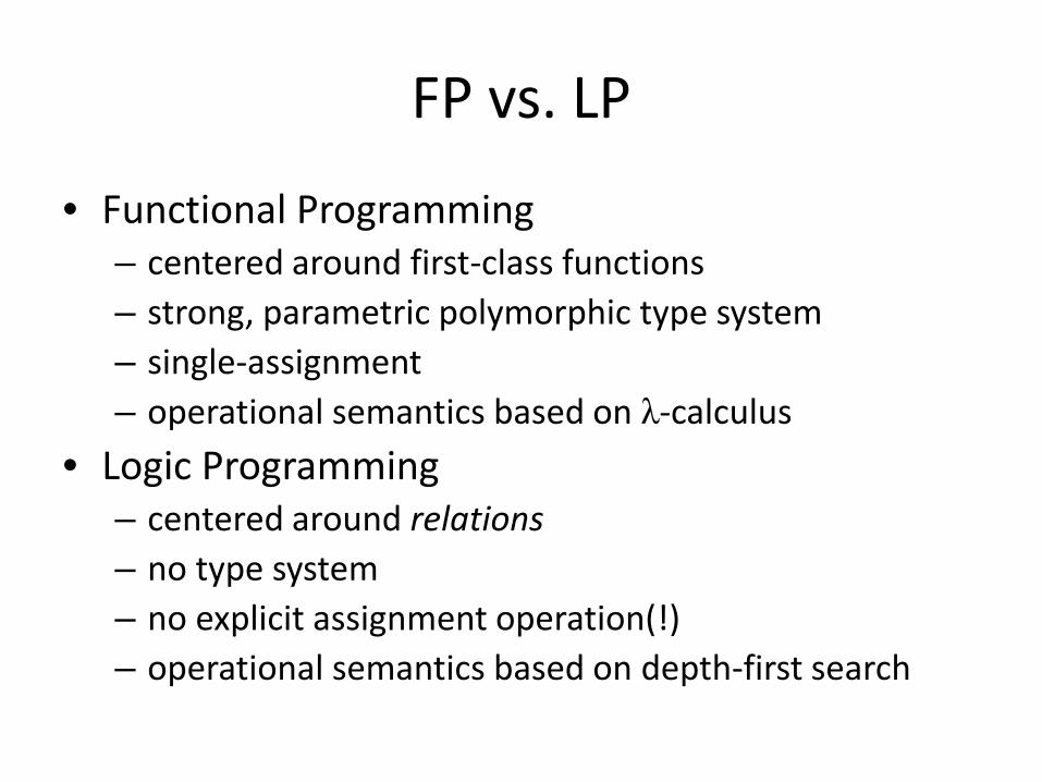
• Functional Programming– centered around first-class functions– strong, parametric polymorphic type system– single-assignment– operational semantics based on λ-calculus

• Logic Programming– centered around relations– no type system– no explicit assignment operation(!)– operational semantics based on depth-first search

Relations

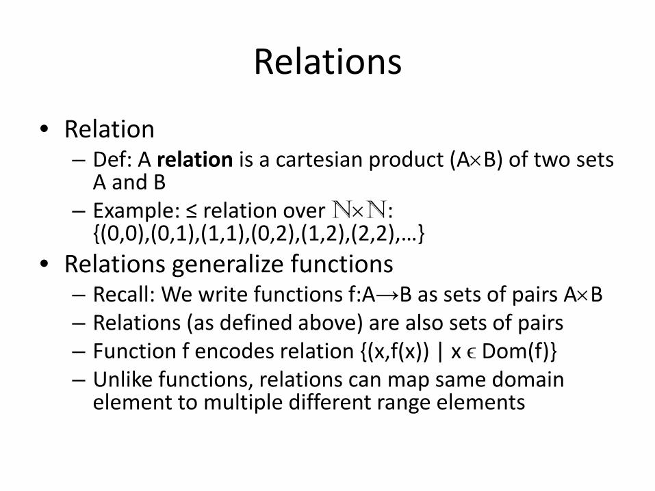
• Relation– Def: A relation is a cartesian product (A×B) of two sets

A and B– Example: ≤ relation over N×N:

{(0,0),(0,1),(1,1),(0,2),(1,2),(2,2),…}• Relations generalize functions

– Recall: We write functions f:A→B as sets of pairs A×B– Relations (as defined above) are also sets of pairs– Function f encodes relation {(x,f(x)) | x ϵ Dom(f)}– Unlike functions, relations can map same domain

element to multiple different range elements

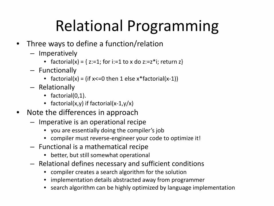
Relational Programming• Three ways to define a function/relation

– Imperatively• factorial(x) = { z:=1; for i:=1 to x do z:=z*i; return z}

– Functionally• factorial(x) = (if x<=0 then 1 else x*factorial(x-1))

– Relationally• factorial(0,1).• factorial(x,y) if factorial(x-1,y/x)

• Note the differences in approach– Imperative is an operational recipe

• you are essentially doing the compiler’s job• compiler must reverse-engineer your code to optimize it!

– Functional is a mathematical recipe• better, but still somewhat operational

– Relational defines necessary and sufficient conditions• compiler creates a search algorithm for the solution• implementation details abstracted away from programmer• search algorithm can be highly optimized by language implementation

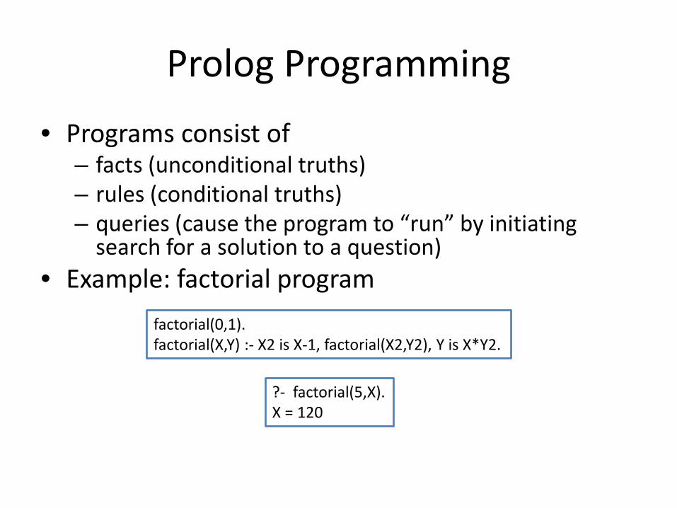
Prolog Programming

• Programs consist of– facts (unconditional truths)– rules (conditional truths)– queries (cause the program to “run” by initiating

search for a solution to a question)• Example: factorial program

factorial(0,1).factorial(X,Y) :- X2 is X-1, factorial(X2,Y2), Y is X*Y2.

?- factorial(5,X).X = 120

Applications

• Originally invited by Robert Kowalski (for theorem-proving) and Alain Colmeraur (for NLP) [1973]

• Now used primarily for– artificial intelligence– scheduling problems– databases (Datalog)– model-checking– compilers– software engineering (verification, etc.)– network protocol analysis– many other applications…

Running Prolog• One Prolog programming assignment (given next time)• Two installation options

– Use CS Dept Unix machines to do assignment, or– Install SWI Prolog on your machine (see link on course web page)

• Programming– create a text file named “lastname.pl”– text file contains facts and rules (no queries)

• Running your program– type “pl” at the Unix prompt– type “consult(lastname).” at Prolog prompt– enter queries at Prolog prompt– to reload after changing programs, just type “make.”– exit by typing control-C then “e”

Prolog Syntax• Each program line has one of two forms:

– p(t1,…,tn).– p(t1,…,tn) :- p1(t1,…,ti), p2(t1,…,tj), …, pm(t1,…,tk).– Don’t forget the period ending each line!– p is a “predicate” consisting of lower-case letters (e.g., “factorial”)– t1,…,tn are “terms”

• Terms can be…– integer constants (1, -13, etc.)– atoms (non-numerical constants)

• consist of lower-case letters or surrounded by single-quotes• Examples: x, abc, ‘Foo’

– variables (start with Capital letters)• Examples: X, Foo

– structures (tree-like data structures)• Examples: foo(3,12), foo(foo(13),foo(16,12))• syntax like predicates but not the same as predicates!• no type system, so be careful!

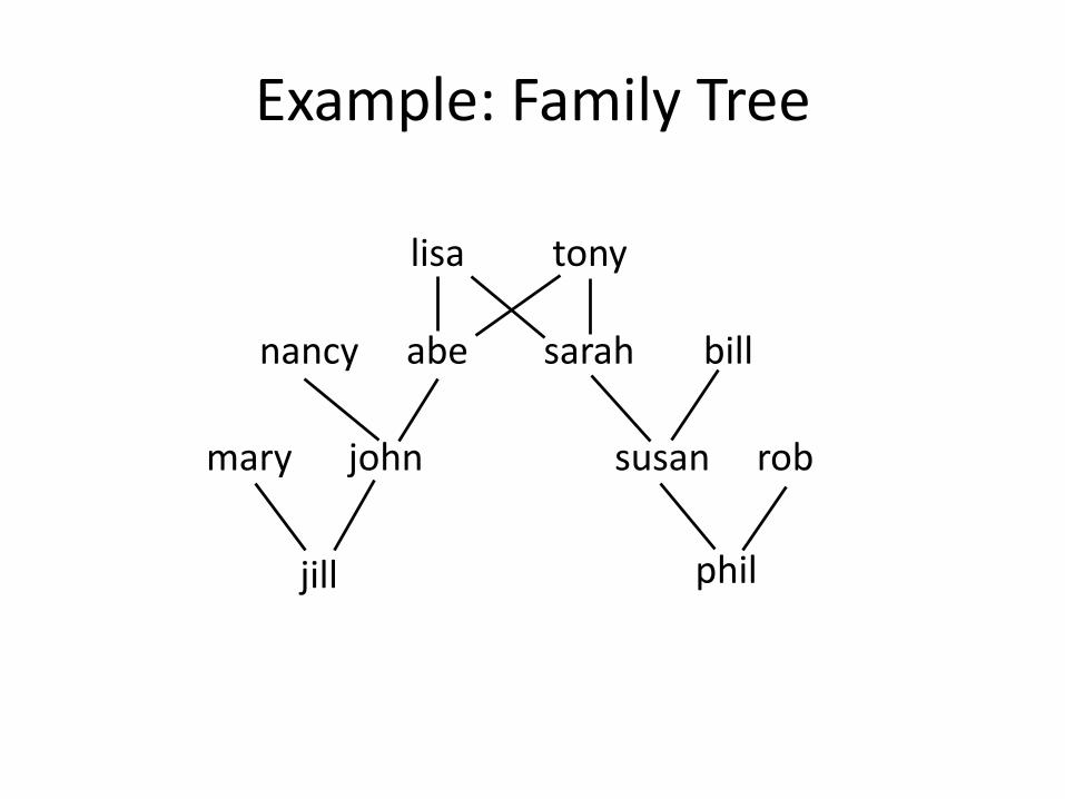
Example: Family Tree

lisa tony

abe sarahnancy bill

johnmary

jill

susan rob

phil

Prolog Representation of Family Tree

father(tony,abe).father(tony,sarah).father(abe,john).father(bill,susan).father(john,jill).father(rob,phil).mother(lisa,abe).mother(lisa,sarah).mother(nancy,john).mother(sarah,susan).mother(mary,jill).mother(susan,phil).

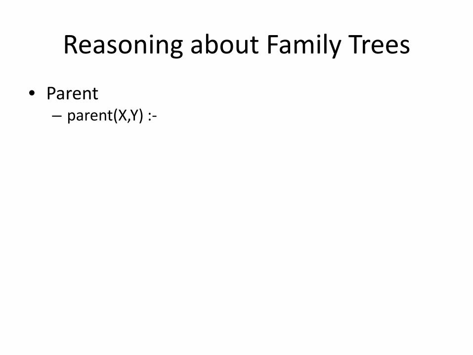
Reasoning about Family Trees

• Parent– parent(X,Y) :-

Reasoning about Family Trees

• Parent– parent(X,Y) :- father(X,Y).– parent(X,Y) :- mother(X,Y).

• Grandparent– gp(X,Y) :-

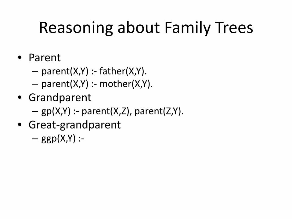
Reasoning about Family Trees

• Parent– parent(X,Y) :- father(X,Y).– parent(X,Y) :- mother(X,Y).

• Grandparent– gp(X,Y) :- parent(X,Z), parent(Z,Y).

• Great-grandparent– ggp(X,Y) :-

Reasoning about Family Trees

• Parent– parent(X,Y) :- father(X,Y).– parent(X,Y) :- mother(X,Y).

• Grandparent– gp(X,Y) :- parent(X,Z), parent(Z,Y).

• Great-grandparent– ggp(X,Y) :- gp(X,Z), parent(Z,Y).

• Ancestor– ancestor(X,Y) :-

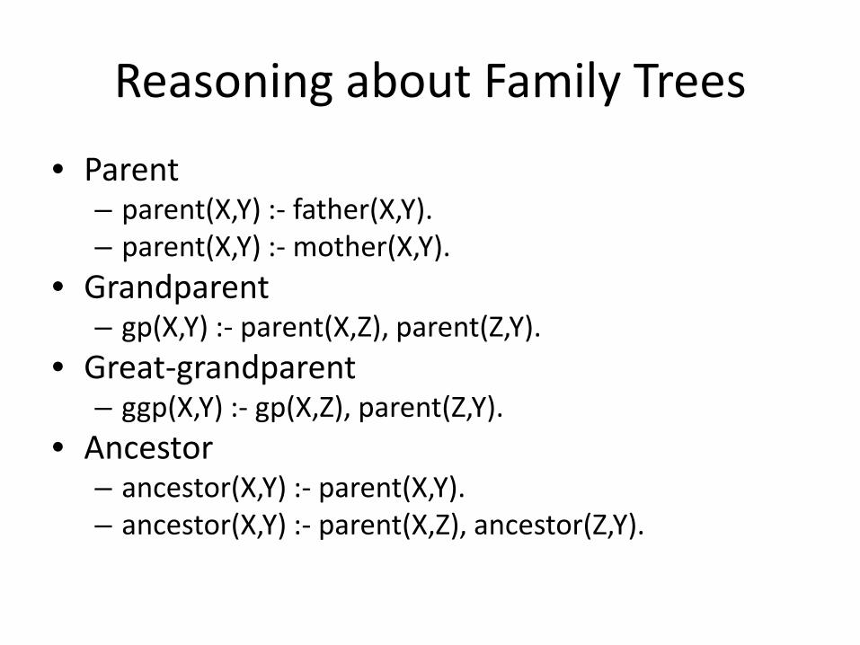
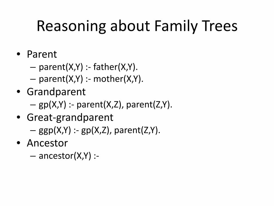
Reasoning about Family Trees

• Parent– parent(X,Y) :- father(X,Y).– parent(X,Y) :- mother(X,Y).

• Grandparent– gp(X,Y) :- parent(X,Z), parent(Z,Y).

• Great-grandparent– ggp(X,Y) :- gp(X,Z), parent(Z,Y).

• Ancestor– ancestor(X,Y) :- parent(X,Y).– ancestor(X,Y) :- parent(X,Z), ancestor(Z,Y).

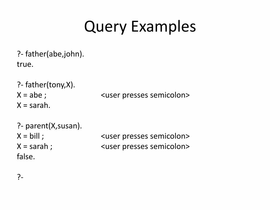
Query Examples?- father(abe,john).true.

?- father(tony,X).X = abe ; <user presses semicolon>X = sarah.

?- parent(X,susan).X = bill ; <user presses semicolon>X = sarah ; <user presses semicolon>false.

?-

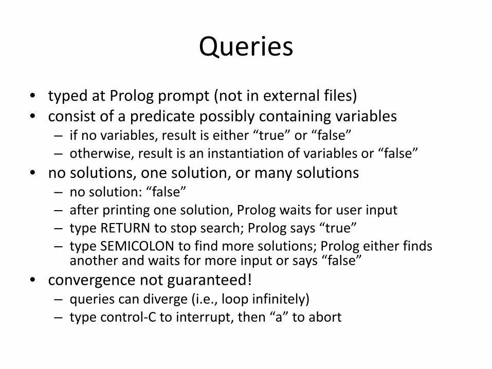
Queries• typed at Prolog prompt (not in external files)• consist of a predicate possibly containing variables

– if no variables, result is either “true” or “false”– otherwise, result is an instantiation of variables or “false”

• no solutions, one solution, or many solutions– no solution: “false”– after printing one solution, Prolog waits for user input– type RETURN to stop search; Prolog says “true”– type SEMICOLON to find more solutions; Prolog either finds

another and waits for more input or says “false”• convergence not guaranteed!

– queries can diverge (i.e., loop infinitely)– type control-C to interrupt, then “a” to abort

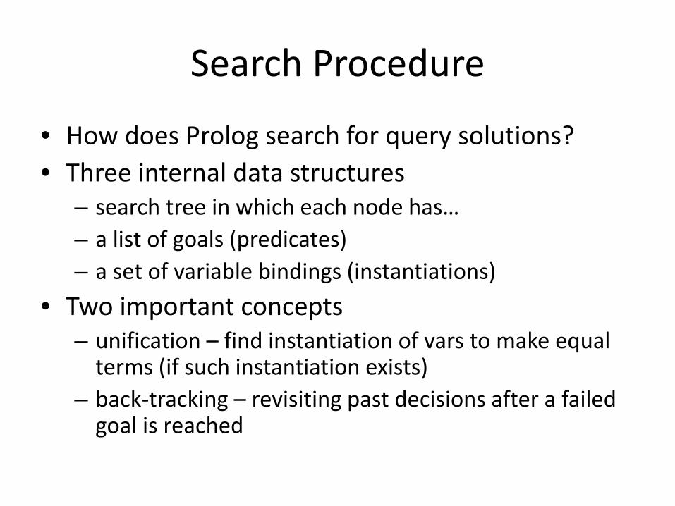
Search Procedure

• How does Prolog search for query solutions?• Three internal data structures

– search tree in which each node has…– a list of goals (predicates)– a set of variable bindings (instantiations)

• Two important concepts– unification – find instantiation of vars to make equal

terms (if such instantiation exists)– back-tracking – revisiting past decisions after a failed

goal is reached

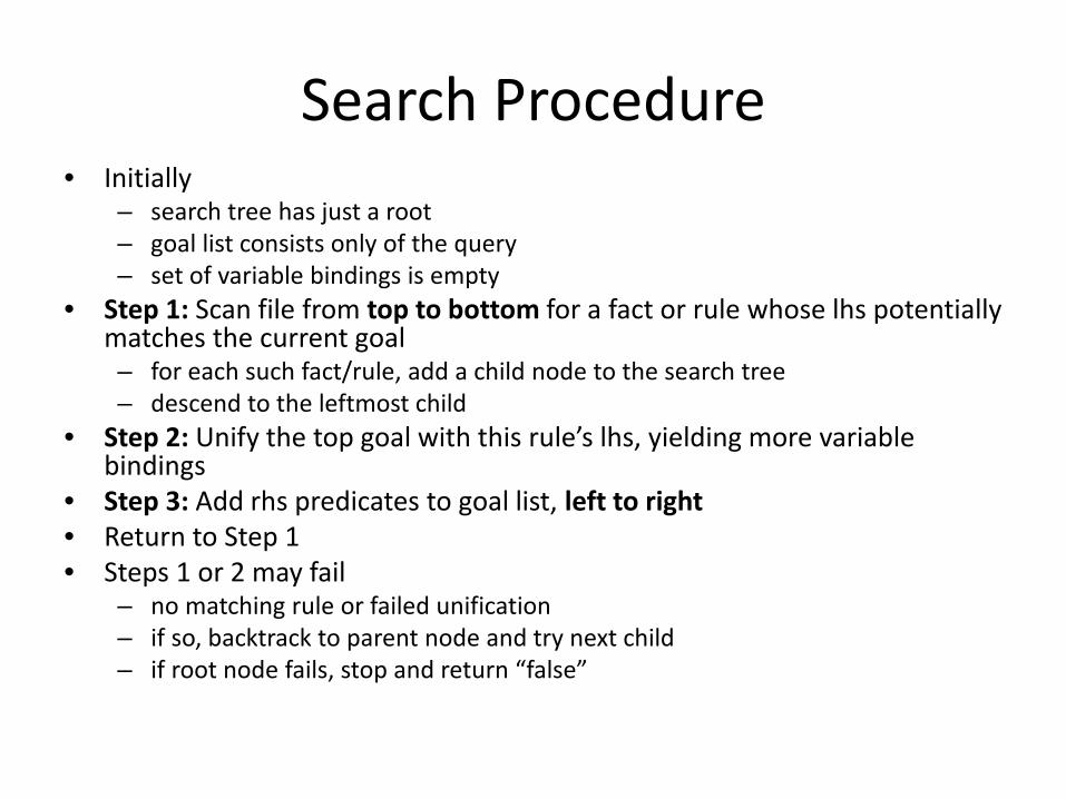
Search Procedure• Initially

– search tree has just a root– goal list consists only of the query– set of variable bindings is empty

• Step 1: Scan file from top to bottom for a fact or rule whose lhs potentially matches the current goal– for each such fact/rule, add a child node to the search tree– descend to the leftmost child

• Step 2: Unify the top goal with this rule’s lhs, yielding more variable bindings

• Step 3: Add rhs predicates to goal list, left to right• Return to Step 1• Steps 1 or 2 may fail

– no matching rule or failed unification– if so, backtrack to parent node and try next child– if root node fails, stop and return “false”

Search Exampleancestor(tony,phil)

ancestor(X1,Y1) :- parent(X1,Y1). ancestor(X1,Y1) :- parent(X1,Z1),ancestor(Z1,Y1).X1=tony, Y1=phil

parent(tony,phil)

parent(X2,Y2) :-father(X2,Y2).

parent(X2,Y2) :-mother(X2,Y2).

X1=X2=tony, Y1=Y2=philfather(tony,phil)

FAILS

X1=X2=tony, Y1=Y2=philmother(tony,phil)

FAILS

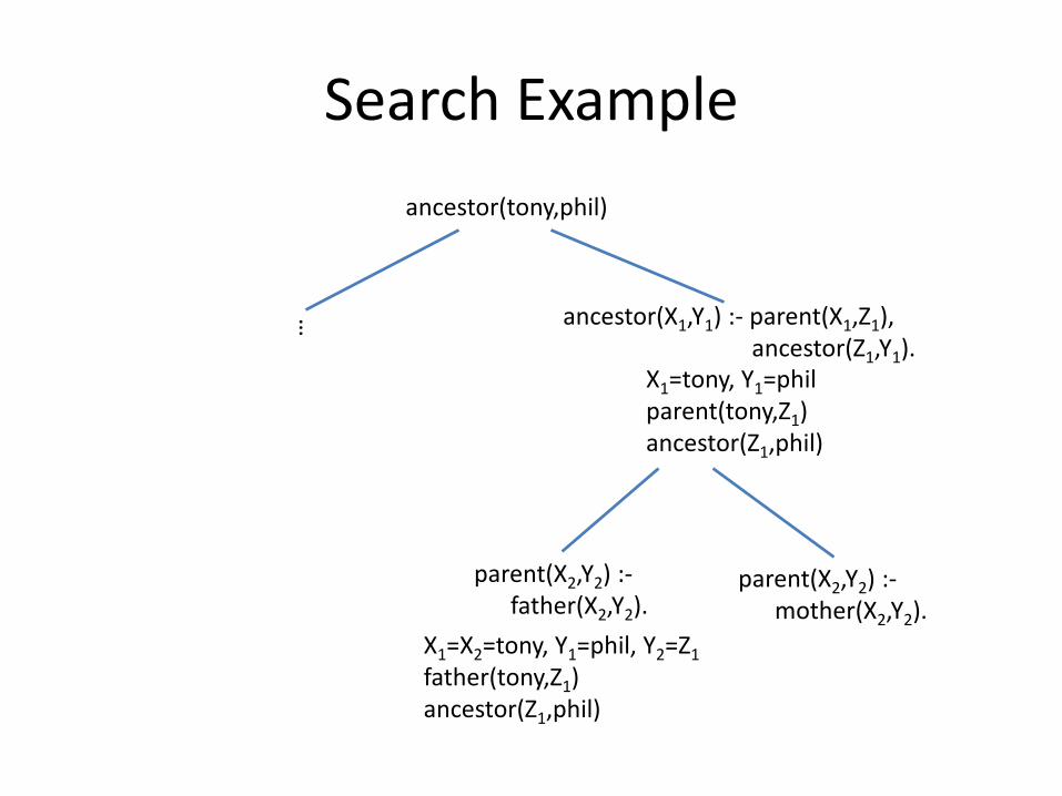
Search Exampleancestor(tony,phil)

ancestor(X1,Y1) :- parent(X1,Z1),ancestor(Z1,Y1).

X1=tony, Y1=philparent(tony,Z1)ancestor(Z1,phil)

…

parent(X2,Y2) :-father(X2,Y2).

parent(X2,Y2) :-mother(X2,Y2).

X1=X2=tony, Y1=phil, Y2=Z1father(tony,Z1)ancestor(Z1,phil)

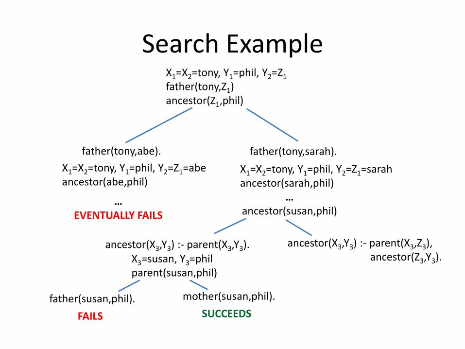
Search ExampleX1=X2=tony, Y1=phil, Y2=Z1father(tony,Z1)ancestor(Z1,phil)

father(tony,abe). father(tony,sarah).X1=X2=tony, Y1=phil, Y2=Z1=abeancestor(abe,phil)

…EVENTUALLY FAILS

X1=X2=tony, Y1=phil, Y2=Z1=sarahancestor(sarah,phil)

…ancestor(susan,phil)

ancestor(X3,Y3) :- parent(X3,Y3). ancestor(X3,Y3) :- parent(X3,Z3),ancestor(Z3,Y3).X3=susan, Y3=phil

parent(susan,phil)

father(susan,phil). mother(susan,phil).

FAILS SUCCEEDS

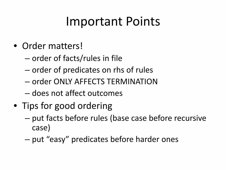
Important Points

• Order matters!– order of facts/rules in file– order of predicates on rhs of rules– order ONLY AFFECTS TERMINATION– does not affect outcomes

• Tips for good ordering– put facts before rules (base case before recursive

case)– put “easy” predicates before harder ones

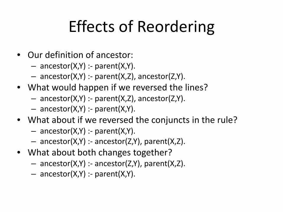
Effects of Reordering• Our definition of ancestor:

– ancestor(X,Y) :- parent(X,Y).– ancestor(X,Y) :- parent(X,Z), ancestor(Z,Y).

• What would happen if we reversed the lines?– ancestor(X,Y) :- parent(X,Z), ancestor(Z,Y).– ancestor(X,Y) :- parent(X,Y).

• What about if we reversed the conjuncts in the rule?– ancestor(X,Y) :- parent(X,Y).– ancestor(X,Y) :- ancestor(Z,Y), parent(X,Z).

• What about both changes together?– ancestor(X,Y) :- ancestor(Z,Y), parent(X,Z).– ancestor(X,Y) :- parent(X,Y).

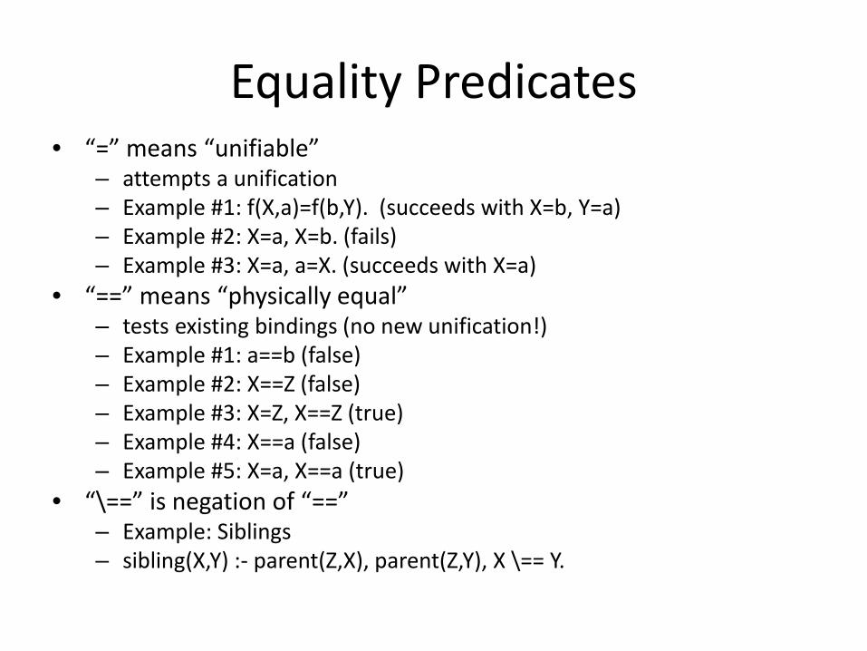
Equality Predicates• “=” means “unifiable”

– attempts a unification– Example #1: f(X,a)=f(b,Y). (succeeds with X=b, Y=a)– Example #2: X=a, X=b. (fails)– Example #3: X=a, a=X. (succeeds with X=a)

• “==” means “physically equal”– tests existing bindings (no new unification!)– Example #1: a==b (false)– Example #2: X==Z (false)– Example #3: X=Z, X==Z (true)– Example #4: X==a (false)– Example #5: X=a, X==a (true)

• “\==” is negation of “==”– Example: Siblings– sibling(X,Y) :- parent(Z,X), parent(Z,Y), X \== Y.

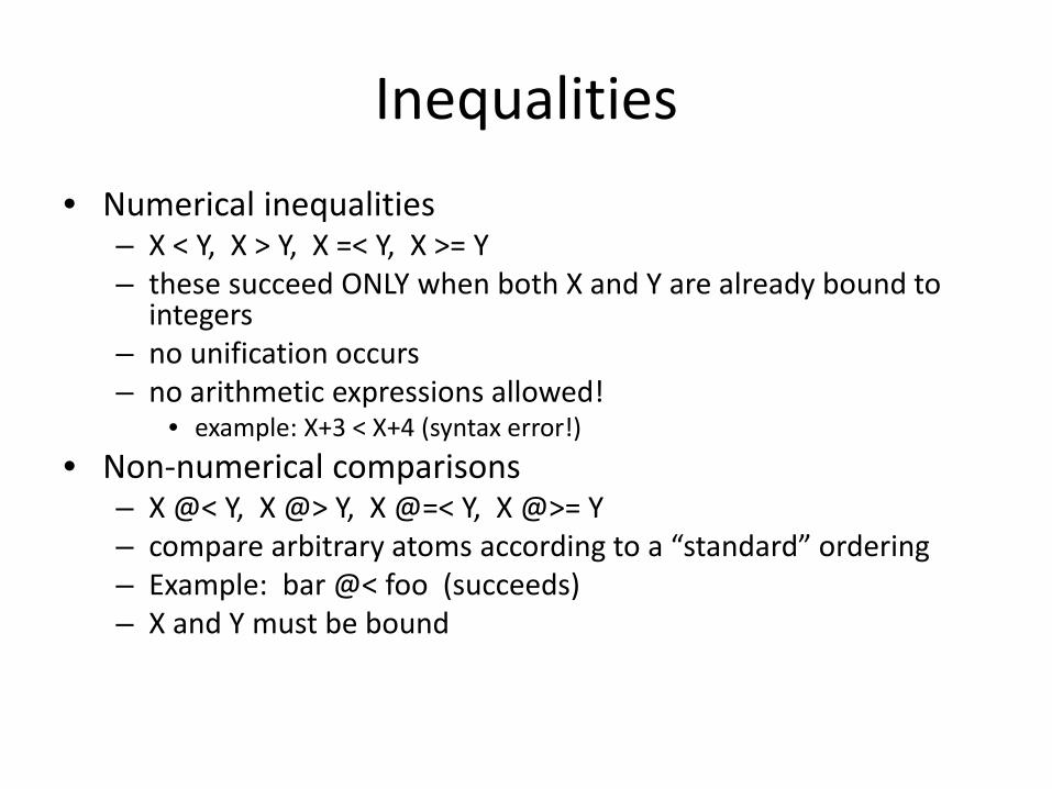
Inequalities• Numerical inequalities

– X < Y, X > Y, X =< Y, X >= Y– these succeed ONLY when both X and Y are already bound to

integers– no unification occurs– no arithmetic expressions allowed!

• example: X+3 < X+4 (syntax error!)• Non-numerical comparisons

– X @< Y, X @> Y, X @=< Y, X @>= Y– compare arbitrary atoms according to a “standard” ordering– Example: bar @< foo (succeeds)– X and Y must be bound

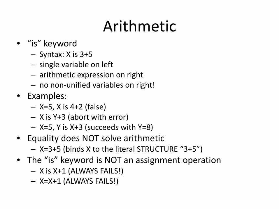
Arithmetic• “is” keyword

– Syntax: X is 3+5– single variable on left– arithmetic expression on right– no non-unified variables on right!

• Examples:– X=5, X is 4+2 (false)– X is Y+3 (abort with error)– X=5, Y is X+3 (succeeds with Y=8)

• Equality does NOT solve arithmetic– X=3+5 (binds X to the literal STRUCTURE “3+5”)

• The “is” keyword is NOT an assignment operation– X is X+1 (ALWAYS FAILS!)– X=X+1 (ALWAYS FAILS!)

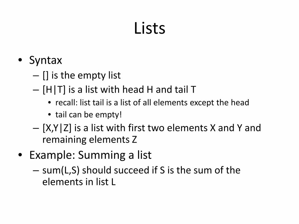
Lists

• Syntax– [] is the empty list– [H|T] is a list with head H and tail T

• recall: list tail is a list of all elements except the head• tail can be empty!

– [X,Y|Z] is a list with first two elements X and Y and remaining elements Z

• Example: Summing a list– sum(L,S) should succeed if S is the sum of the

elements in list L

Lists

• Syntax– [] is the empty list– [H|T] is a list with head H and tail T

• recall: list tail is a list of all elements except the head• tail can be empty!

– [X,Y|Z] is a list with first two elements X and Y and remaining elements Z

• Example: Summing a list– sum([],0).– sum([H|T],S) :- sum(T,S1), S is H+S1.

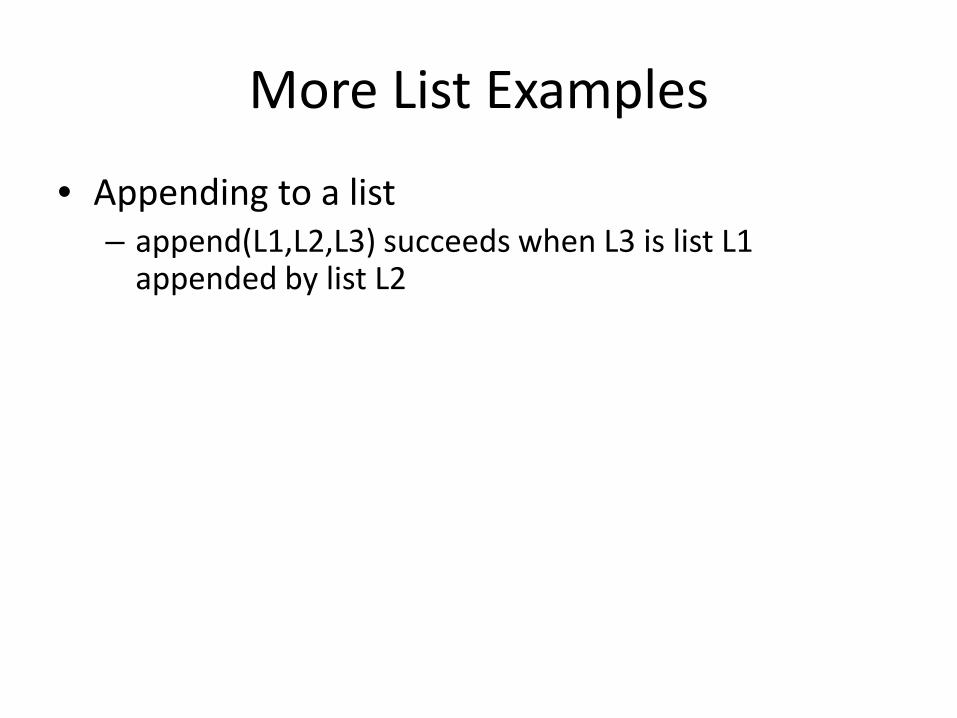
More List Examples

• Appending to a list– append(L1,L2,L3) succeeds when L3 is list L1

appended by list L2

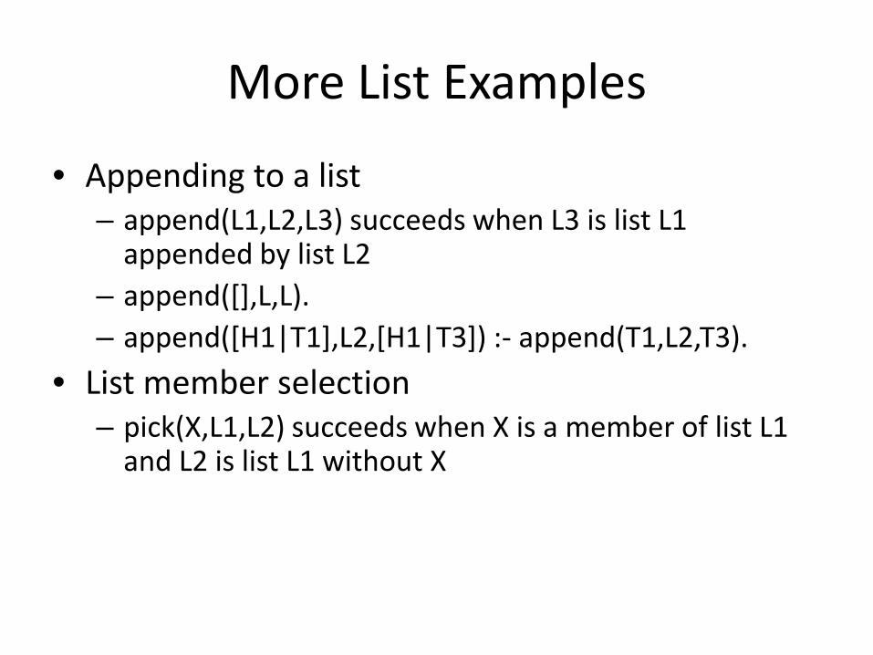
More List Examples

• Appending to a list– append(L1,L2,L3) succeeds when L3 is list L1

appended by list L2– append([],L,L).– append([H1|T1],L2,[H1|T3]) :- append(T1,L2,T3).

• List member selection– pick(X,L1,L2) succeeds when X is a member of list L1

and L2 is list L1 without X

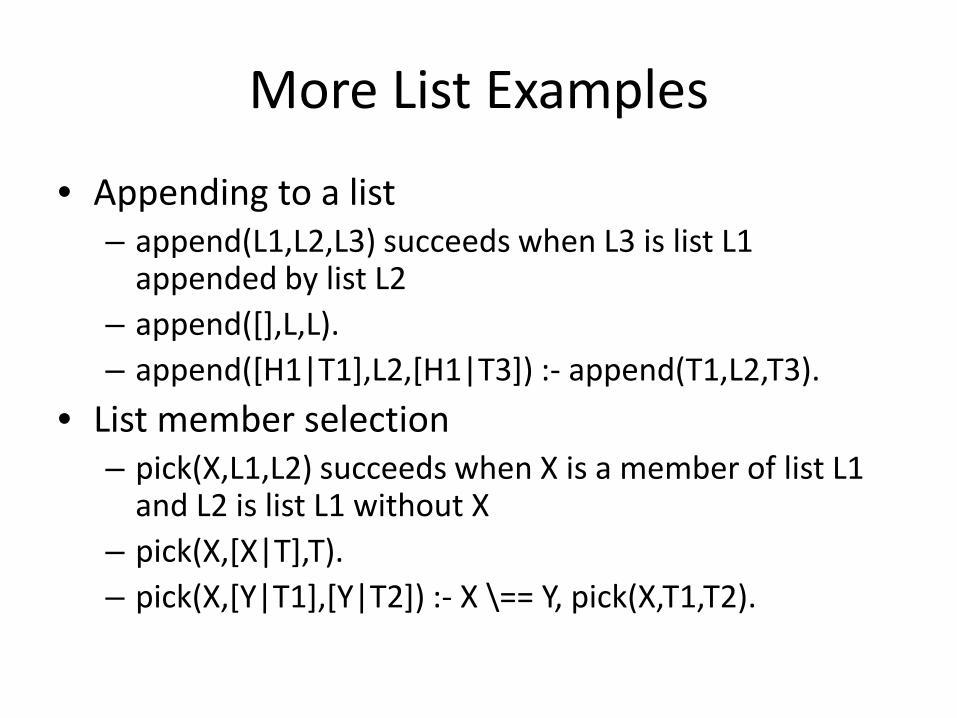
More List Examples

• Appending to a list– append(L1,L2,L3) succeeds when L3 is list L1

appended by list L2– append([],L,L).– append([H1|T1],L2,[H1|T3]) :- append(T1,L2,T3).

• List member selection– pick(X,L1,L2) succeeds when X is a member of list L1

and L2 is list L1 without X– pick(X,[X|T],T).– pick(X,[Y|T1],[Y|T2]) :- X \== Y, pick(X,T1,T2).

Logical Arithmetic

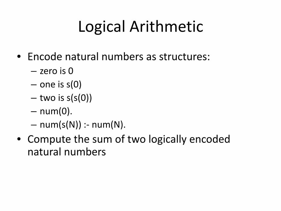
• Encode natural numbers as structures:– zero is 0– one is s(0)– two is s(s(0))– num(0).– num(s(N)) :- num(N).

• Compute the sum of two logically encoded natural numbers

Logical Arithmetic

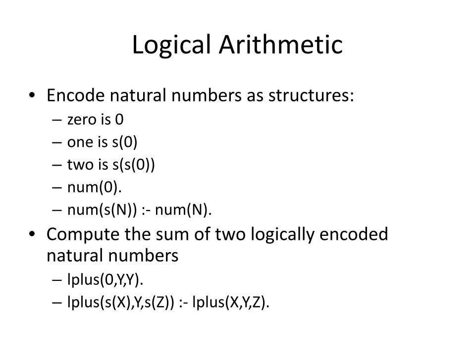
• Encode natural numbers as structures:– zero is 0– one is s(0)– two is s(s(0))– num(0).– num(s(N)) :- num(N).

• Compute the sum of two logically encoded natural numbers– lplus(0,Y,Y).– lplus(s(X),Y,s(Z)) :- lplus(X,Y,Z).

Logical Arithmetic

• Logical subtraction

Logical Arithmetic

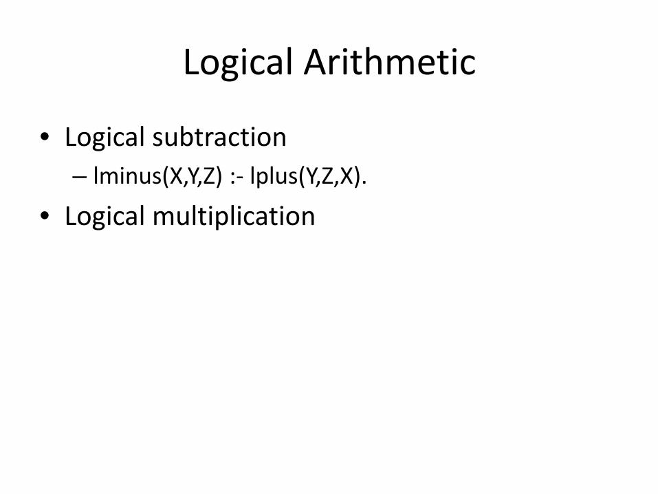
• Logical subtraction– lminus(X,Y,Z) :- lplus(Y,Z,X).

• Logical multiplication

Logical Arithmetic

• Logical subtraction– lminus(X,Y,Z) :- lplus(Y,Z,X).

• Logical multiplication– ltimes(0,Y,0).– ltimes(s(X),Y,Z) :- ltimes(X,Y,XY), lplus(XY,Y,Z).

Negation

• \+ P– succeeds when predicate P terminates with failure– NOT the same as logical negation!– think of it more like “P is disprovable”– loops when P loops– exacerbates order-sensitivity issues– avoid spurious uses

Misc. Operators• semicolon is “or”

– parent(X,Y) :- (father(X,Y); mother(X,Y)), X \== Y– never needed but can make rules shorter

• Underscore is a wildcard– len([],0).– len([_|T],X) :- len(T,Y), X is Y+1.– If you write “[H|T]” instead of “[_|T]”, you’ll get a warning

because H is defined but never used.– Warnings are to help you identify typos (e.g., mistyped variable

names).• Other operators available as well

– see online Prolog documentation (linked from website)– not needed for this class, but you can use them if you wish