lipn.univ-paris13.frgmanzonetto/papers/dmp13.pdflipn.univ-paris13.fr

Call-by-Value Non-determinismin a Linear Logic Type Discipline

Alejandro Dıaz-Caro1,?, Giulio Manzonetto1,2, and Michele Pagani1,2

1 Universite Paris 13, Sorbonne Paris Cite, LIPN, F-93430, Villetaneuse, France2 CNRS, UMR 7030, F-93430, Villetaneuse, France

Abstract. We consider the call-by-value λ-calculus extended with amay-convergent non-deterministic choice and a must-convergent parallelcomposition. Inspired by recent works on the relational semantics of lin-ear logic and non-idempotent intersection types, we endow this calculuswith a type system based on the so-called Girard’s second translation ofintuitionistic logic into linear logic. We prove that a term is typable ifand only if it is converging, and that its typing tree carries enough infor-mation to give a bound on the length of its lazy call-by-value reduction.Moreover, when the typing tree is minimal, such a bound becomes theexact length of the reduction.

1 Introduction

The intersection type discipline provides logical characterisations of operationalproperties of λ-terms, namely of various notions of termination, like head-, weak-and strong-normalisation (see [1, 2], and [3] as a reference). The basic idea is tolook at types as the set of terms having a given computational property — thetype α ∩ β being the set of those terms enjoying both properties α and β. Withthis intuition in mind, the intersection is naturally idempotent (α ∩ α = α).

Another way to understand the intersection type discipline is as a deductivesystem for presenting the compact elements of a specific reflexive Scott domain(see e.g. [4, §3.3]). The set of types assigned to a closed term captures the inter-pretation of such a term in the associated domain. Intersection types are thena powerful tool for enlightening the relations between denotational semantics,syntactical types and computational properties of programs.

Intersection types have been recently revisited in the setting of the relationalsemantics Rel of Linear Logic (LL). Rel is a semantics providing a more quanti-tative interpretation of the λ-calculus than Scott domains. Loosely speaking, therelational interpretation of a λ-term M not only tells us whether M convergeson an argument, but in case it does, it also provides information on the numberof times M needs to call3 its argument to converge. Just like the intersectiontype discipline captures Scott domains, non-idempotent intersection type sys-tems represent relational models. In this framework the type α1 ∩ · · · ∩ αk may

? Partially supported by grants from DIGITEO and Region Ile-de-France.3 The notion of calling an argument should be made precise by specifying an opera-

tional semantics, which is usually achieved through an evaluating machine.

2 Alejandro Dıaz-Caro, Giulio Manzonetto, and Michele Pagani

be more accurately represented as the finite multiset [α1, . . . , αk]. The lack ofidempotency is the key ingredient to model the resource sensitiveness of Rel —while in the usual systems M : α ∩ β stands for “M can be used either as dataof type α or as data of type β”, when the intersection is not idempotent themeaning of M : [α, β] becomes “M will be called once as data of type α andonce as data of type β”. Hence, types should no longer be understood as sets ofterms, but rather as sets of calls to terms.

The first intersection type system based on Rel has been presented in [5],where de Carvalho introduced system R, a type discipline capturing the re-lational version of Engeler’s model. More precisely, he proved that system R,beyond characterising converging terms, carries information on the evaluationsequence as well — the size of a derivation tree typing a term is a bound onthe number of steps needed to reach a normal form. Similar results are obtainedin [6] for a variant of system R characterising strong normalisation and giving abound to the longest β-reduction sequence. More recently, Ehrhard introduceda non-idempotent intersection type system characterising the convergence in thecall-by-value λ-calculus [7]. Also in this case, the size of a derivation tree boundsthe length of the lazy (i.e. no evaluation under λ’s) call-by-value β-reductionsequence. Our goal is to extend Ehrhard’s system with non-determinism.

Our starting point is [8], where it is shown that the relational model D of thecall-by-name λ-calculus provides a natural interpretation of both may and mustnon-determinism. Since Rel interprets λ-terms as relations, the may-convergentnon-deterministic choice can be expressed in the model as the set-theoreticalunion. The must-convergent parallel composition, instead, is interpreted by usingthe operation D⊗D( D obtained by combining the mix rule D⊗D( D`Dwith the contraction rule D`D( D, this latter holding since the call-by-namemodel D has shape ?A for A = DN (⊥. We will show that the same principle(may-convergence as union of interpretations and must-convergence as mix ruleplus contraction) still works in the call-by-value setting.

Ehrhard’s call-by-value type system is based on the so-called “second Girard’stranslation” of intuitionistic logic into LL [9, 10]. The translation of a type αis actually given by two mutually defined mappings (α 7→ αv and α 7→ αc)reflecting the two sorts (values and computations) at the basis of the call-by-value λ-calculus:

ιv = ι, (α→ β)v = αc ( βc, αc = !αv,

where ι is an atom. Hence, the relational model described by Ehrhard’s typingsystem yields a solution to the equation V ' !V ( !V in Rel. Since in thissemantics ( is interpreted by the cartesian product and ! by finite multisets,a functional type for a value in this system is a pair (p, q) of types for compu-tations, and a type for a computation is a multiset [α1, . . . , αn] of value types(representing n calls to a single value that must behave as α1, . . . , αn).

In order to deal with the must non-determinism, namely the parallel composi-tion, we must add to the translation considered by Ehrhard a further exponential

Call-by-Value Non-determinism in a Linear Logic Type Discipline 3

level, called here the parallel sort :

ιv = ι, (α→ β)v = αc ( β‖, αc = !αv, α‖ = ?αc. (1)

This translation enjoys the nice property of mapping the call-by-value λ-calculusinto the polarised fragment of LL, as described by Laurent in [11]. Then, our typ-ing system is describing an object in Rel satisfying the equation V ' !V ( ?!V,where the ? connective is interpreted by the finite multiset operator. In thissetting a value type is a pair (p, [q1, . . . , qn]) of a computational type p and aparallel type, that is a multiset of computations q1, . . . , qn. Intuitively, a valueof that type needs a computation of type p to create a parallel compositionof n computations of types q1, . . . , qn, respectively. Notice that, following [8],the composition of the mix rule and the contraction one yields an operation?!V ⊗ ?!V ( ?!V which is used to interpret the parallel composition.

To avoid a clumsy notation with multisets of multisets, we prefer to denotea !-multiset [α1, . . . , αm] (the type of a computation) with the linear logic multi-plicative conjunction α1⊗· · ·⊗αm, a ?-multiset [q1, . . . , qn] (the type of a parallelcomposition of computations) with the multiplicative disjunction q1 ` · · ·` qn,and finally a pair (p, [q1, . . . , qn]) with the linear implication p( (q1 ` · · ·` qn).Such a notation stresses the fact that the non-idempotent intersection type sys-tems issued from Rel are essentially contained in the multiplicative fragment ofLL (modulo the associativity, commutativity and neutrality equivalences).

Contents. Several non-deterministic extensions of the λ-calculus have beenproposed in the literature, both in the call-by-name (e.g. [8, 12]) and in the call-by-value setting (e.g. [13, 14]). In the present paper we focus on the call-by-valueλ-calculus, first introduced in [15], endowed with two binary operators + and ‖representing non-deterministic choice and parallel composition, respectively. Theresulting calculus, denoted here Λ+‖, is quite standard and its operational seman-tics is given in Section 2 through a machine performing lazy call-by-value reduc-tion. Following [8], we model non-deterministic choice as may non-determinismand parallel composition as must. This is reflected in our reduction and in ournotion of convergence. Indeed, every time the machine encounters M + N inactive position it actually performs a choice, while encountering M ‖ N it in-terleaves reductions in M and in N ; finally a term M converges when there is areduction of the machine from M to a normal form.

Section 3 is devoted to provide the type discipline for Λ+‖, based on themultiplicative fragment of LL (as discussed above), and to define a measure | · |associating a number with every type derivation. Such a measure “extracts” fromthe information present in the typing tree of a term, a bound on the length of itsevaluation. In Section 4 we show that our type system satisfies good propertieslike subject reduction and expansion. We also prove that the measure associatedwith the typing tree of a term decreases by 1 at every reduction step, giving thusa proof of weak normalisation in ω for typable terms. From these properties itensues directly that a term is typable if and only if it converges. Moreover, thanksto the resource consciousness of our type system, we are able to strengthen such aresult — we prove that, wheneverM converges, there is a type derivation `M : α


βv-reduction +-reductions ‖-reductions(λx.M)V →M [V/x] M +N →M

M +N → N(M ‖ N)P →MP ‖ NPV (M ‖ N)→ VM ‖ V N

Contextual rules

M →M ′

M ‖ N →M ′ ‖ N

N → N ′

M ‖ N →M ‖ N ′

M →M ′ (∗)

MN →M ′N

M →M ′ (∗)

VM → VM ′

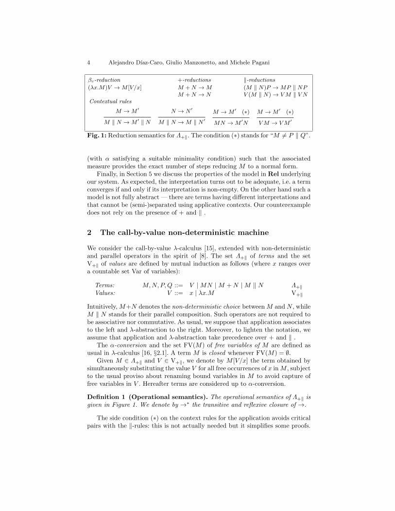
Fig. 1: Reduction semantics for Λ+‖. The condition (∗) stands for “M 6= P ‖ Q”.

(with α satisfying a suitable minimality condition) such that the associatedmeasure provides the exact number of steps reducing M to a normal form.

Finally, in Section 5 we discuss the properties of the model in Rel underlyingour system. As expected, the interpretation turns out to be adequate, i.e. a termconverges if and only if its interpretation is non-empty. On the other hand such amodel is not fully abstract — there are terms having different interpretations andthat cannot be (semi-)separated using applicative contexts. Our counterexampledoes not rely on the presence of + and ‖ .

2 The call-by-value non-deterministic machine

We consider the call-by-value λ-calculus [15], extended with non-deterministicand parallel operators in the spirit of [8]. The set Λ+‖ of terms and the setV+‖ of values are defined by mutual induction as follows (where x ranges overa countable set Var of variables):

Terms: M,N,P,Q ::= V |MN |M +N |M ‖ N Λ+‖Values: V ::= x | λx.M V+‖

Intuitively, M+N denotes the non-deterministic choice between M and N , whileM ‖ N stands for their parallel composition. Such operators are not required tobe associative nor commutative. As usual, we suppose that application associatesto the left and λ-abstraction to the right. Moreover, to lighten the notation, weassume that application and λ-abstraction take precedence over + and ‖ .

The α-conversion and the set FV(M) of free variables of M are defined asusual in λ-calculus [16, §2.1]. A term M is closed whenever FV(M) = ∅.

Given M ∈ Λ+‖ and V ∈ V+‖, we denote by M [V/x] the term obtained bysimultaneously substituting the value V for all free occurrences of x inM , subjectto the usual proviso about renaming bound variables in M to avoid capture offree variables in V . Hereafter terms are considered up to α-conversion.

Definition 1 (Operational semantics). The operational semantics of Λ+‖ isgiven in Figure 1. We denote by →∗ the transitive and reflexive closure of →.

The side condition (∗) on the context rules for the application avoids criticalpairs with the ‖-rules: this is not actually needed but it simplifies some proofs.


A term M is called a normal form if there is no N ∈ Λ+‖ such that M → N .In particular, all (parallel compositions of) values are normal forms. Note thatwhen M is closed then either it is a parallel composition of values or it reduces.

Definition 2. A closed term M ∈ Λ+‖ converges if and only if there exists areduction M →∗ V1 ‖ · · · ‖ Vn for some Vi ∈ V+‖.

The intuitive idea underlying the above notion of convergence is the following:

– The non-deterministic choice M +N is treated as may-convergent, either ofthe alternatives may be chosen during the reduction and the sum convergesif either M or N does.

– The parallel composition M ‖ N is modelled as must-convergent, the reduc-tion forks and the parallel composition converges if both M and N do.

Let us provide some examples. We set I = λx.x, ∆ = λx.xx and we denoteby Ω the paradigmatic non-converging term ∆∆, which reduces to itself as∆ is a value. The reduction is lazy, i.e. it does not reduce under abstractions,so for example λy.Ω is a normal form. In fact, when considering closed terms,the parallel compositions of values are exactly the normal forms, thus justifyingDefinition 2. We would like to stress that our system is designed in such away that a parallel composition of values is not a value. As a consequence,the term P = λk.∆ ‖ ∆ is not a value, so the term (λx.xIx)P is converging.Indeed, it reduces to (λx.xIx)(λk.∆) ‖ (λx.xIx)∆ →∗ ∆ ‖ ∆. Notice that, ifwe consider P as a value, then (λx.xIx)P would diverge since it would reduceto P IP →∗ (∆ ‖ I)P →∗ ∆P ‖ P and one can check easily that ∆P diverges.

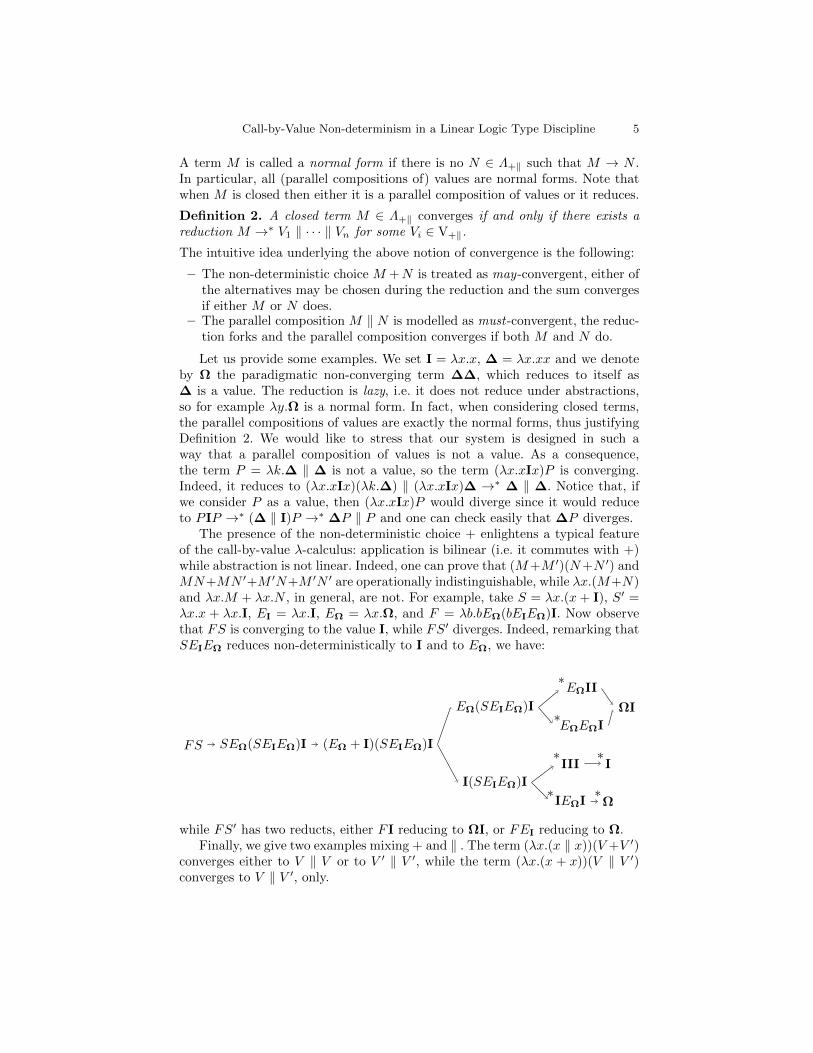
The presence of the non-deterministic choice + enlightens a typical featureof the call-by-value λ-calculus: application is bilinear (i.e. it commutes with +)while abstraction is not linear. Indeed, one can prove that (M+M ′)(N+N ′) andMN+MN ′+M ′N+M ′N ′ are operationally indistinguishable, while λx.(M+N)and λx.M + λx.N , in general, are not. For example, take S = λx.(x+ I), S′ =λx.x + λx.I, EI = λx.I, EΩ = λx.Ω, and F = λb.bEΩ(bEIEΩ)I. Now observethat FS is converging to the value I, while FS′ diverges. Indeed, remarking thatSEIEΩ reduces non-deterministically to I and to EΩ, we have:

FS SEΩ(SEIEΩ)I (EΩ + I)(SEIEΩ)I

EΩ(SEIEΩ)I

EΩII

EΩEΩI

ΩI

I(SEIEΩ)I

III I

IEΩI Ω

∗

∗

∗ ∗

∗ ∗

while FS′ has two reducts, either F I reducing to ΩI, or FEI reducing to Ω.Finally, we give two examples mixing + and ‖ . The term (λx.(x ‖ x))(V +V ′)

converges either to V ‖ V or to V ′ ‖ V ′, while the term (λx.(x + x))(V ‖ V ′)converges to V ‖ V ′, only.


axx : τ ` x : τ

∆i, x : τi `M : αi 1 ≤ i ≤ n(I n ≥ 0

n⊗i=1

∆i ` λx.M :

n⊗i=1

(τi ( αi)

∆ `M :k

i=1

ni⊗j=1

(τij ( αij) Γi ` N :ni

j=1

τij 1 ≤ i ≤ k

(Ek ≥ 1ni ≥ 1

∆⊗k⊗

i=1

Γi `MN :k

i=1

ni

j=1

αij

∆ `M : α+`

∆ `M +N : α

∆ ` N : α+r

∆ `M +N : α

∆ `M : α1 Γ ` N : α2

‖I∆⊗ Γ `M ‖ N : α1 ` α2

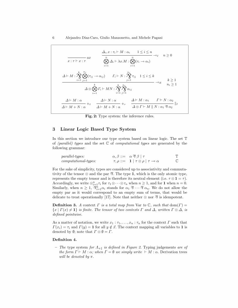
Fig. 2: Type system: the inference rules.

3 Linear Logic Based Type System

In this section we introduce our type system based on linear logic. The set Tof (parallel) types and the set C of computational types are generated by thefollowing grammar:

parallel-types: α, β ::= α` β | τ Tcomputational-types: τ, ρ ::= 1 | τ ⊗ ρ | τ ( α C

For the sake of simplicity, types are considered up to associativity and commuta-tivity of the tensor ⊗ and the par `. The type 1, which is the only atomic type,represents the empty tensor and is therefore its neutral element (i.e. τ ⊗ 1 = τ).Accordingly, we write ⊗n

i=1τi for τ1⊗· · ·⊗τn when n ≥ 1, and for 1 when n = 0.Similarly, when n ≥ 1, `n

i=1αi stands for α1 ` · · · ` αn. We do not allow theempty par as it would correspond to an empty sum of terms, that would bedelicate to treat operationally [17]. Note that neither ⊗ nor ` is idempotent.

Definition 3. A context Γ is a total map from Var to C, such that dom(Γ ) =x | Γ (x) 6= 1 is finite. The tensor of two contexts Γ and ∆, written Γ ⊗∆, isdefined pointwise.

As a matter of notation, we write x1 : τ1, . . . , xn : τn for the context Γ such thatΓ (xi) = τi and Γ (y) = 1 for all y /∈ ~x. The context mapping all variables to 1 isdenoted by ∅; note that Γ ⊗ ∅ = Γ .

Definition 4.

– The type system for Λ+‖ is defined in Figure 2. Typing judgements are ofthe form Γ `M : α; when Γ = ∅ we simply write `M : α. Derivation treeswill be denoted by π.


– A term M ∈ Λ+‖ is typable if there exist α ∈ T and a context Γ such thatΓ `M : α.

The rules for typing non-deterministic choice and parallel composition reflecttheir operational behaviour. Non-deterministic choice is may-convergent, thus itis enough to ask that one of the terms in a sum is typable; on the other handparallel composition is must-convergent, we therefore require that all its compo-nents are typable. Intuitively, when dealing with closed terms, the ` operatorcan be only introduced to type a parallel composition, and gives an accountof the number of its components. In fact, for closed regular λ-terms, the typesystem looses the `-level and collapses to the one presented in [7].

The (E rule reflects the distribution of the parallel operator over the appli-cation. For example, takeM = x ‖ x′ andN = y ‖ y′ in the premises of (E , thenwe have k = 2 and n1 = n2 = 2 so that the type of the term MN is a ` of fourtypes, which is in accordance with (x ‖ x′)(y ‖ y′)→∗ (xy ‖ xy′) ‖ (x′y ‖ x′y′).

Remark 5 For every V ∈ V+‖ we can derive ` V : 1. Indeed, if V is a variable,then the derivation follows by ax; if V is an abstraction, then it follows by (I

using n = 0. As a simple consequence we get ` V1 ‖ · · · ‖ Vk : 1 ` · · · ` 1(k times) for all V1, . . . , Vk ∈ V+‖.

Concerning the possible types of values, the next more general lemma holds.

Lemma 6. Let V ∈ V+‖. If ∆ ` V : α then α ∈ C.

Proof. A proof of ∆ ` V : α ends in either a ax or a (I rule. In both cases αis a computational-type. ut

To help the reader to get familiar with the type system, we provide someexamples of typable and untypable terms.

Example 7. Recall that I = λx.x, ∆ = λx.xx and Ω = ∆∆.

1. ` I :⊗n

i=1(τi ( τi) and ` λx.I :⊗n

i=1(1 (⊗ki

j=1(τij ( τij)).

2. `∆ :⊗n

i=1((τi ( αi)⊗ τi) ( αi.3. Ω is not typable. By contradiction, suppose ` Ω : α. By ((E) and (2) there

is a type τ such that ` ∆ : τ ( α and ` ∆ : τ . Let us choose such a τwith minimal size. Applying (2) to `∆ : τ ( α, we get τ = (τ ′ ( α)⊗ τ ′,from which one can deduce (see Lemma 9, below) that ` ∆ : τ ′ ( α and`∆ : τ ′, thus contradicting the minimality of τ .

4. However, ` λx.Ω : 1, so ` λx.Ω + Ω : 1, but λx.Ω ‖ Ω is not typable.5. From (1) and (4) we get: ` I ‖ λx.Ω : (

⊗ni=1(τi ( τi)) ` 1.

We now define a measure associating a natural number with every derivationtree. In Section 4.1 we prove that such a measure decreases along the reduction.In the next definition we follow the notation of Figure 2, in particular in the(E-case the parameter ni refers to the arity of the

˙in the conclusion of πi.


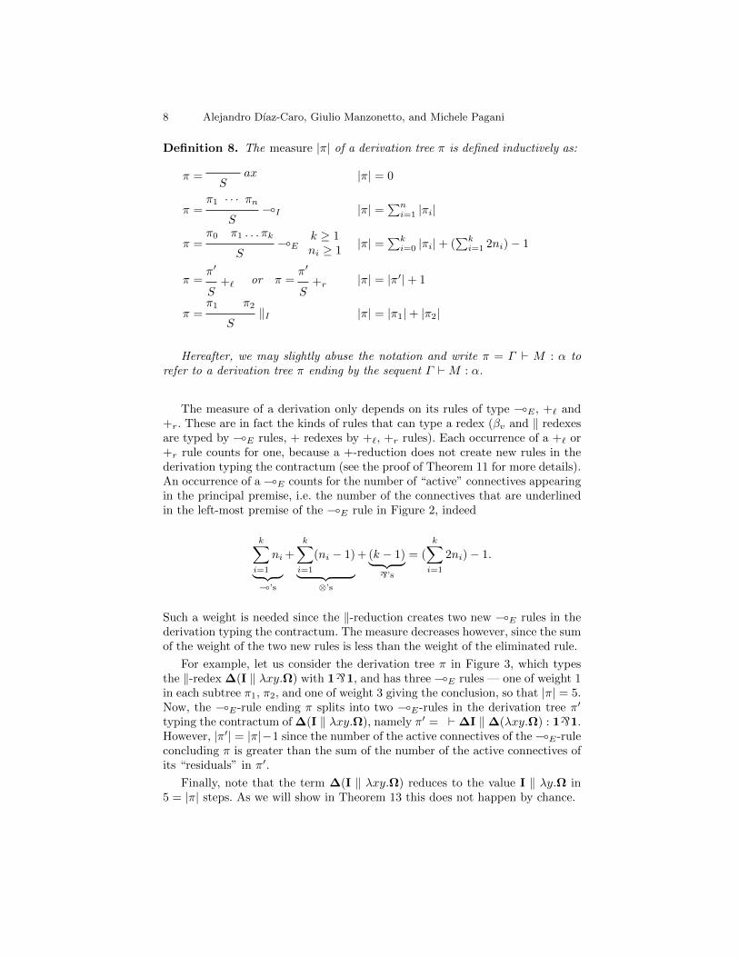
Definition 8. The measure |π| of a derivation tree π is defined inductively as:

π = axS

|π| = 0

π =π1 · · · πn

(IS

|π| =∑n

i=1 |πi|

π =π0 π1 . . . πk

(Ek ≥ 1ni ≥ 1S

|π| =∑k

i=0 |πi|+ (∑k

i=1 2ni)− 1

π =π′

+`S

or π =π′

+rS

|π| = |π′|+ 1

π =π1 π2

‖IS

|π| = |π1|+ |π2|

Hereafter, we may slightly abuse the notation and write π = Γ ` M : α torefer to a derivation tree π ending by the sequent Γ `M : α.

The measure of a derivation only depends on its rules of type (E , +` and+r. These are in fact the kinds of rules that can type a redex (βv and ‖ redexesare typed by (E rules, + redexes by +`, +r rules). Each occurrence of a +` or+r rule counts for one, because a +-reduction does not create new rules in thederivation typing the contractum (see the proof of Theorem 11 for more details).An occurrence of a (E counts for the number of “active” connectives appearingin the principal premise, i.e. the number of the connectives that are underlinedin the left-most premise of the (E rule in Figure 2, indeed

k∑i=1

ni︸︷︷︸(’s

+

k∑i=1

(ni − 1)︸︷︷︸⊗’s

+ (k − 1)︸︷︷︸`’s

= (

k∑i=1

2ni)− 1.

Such a weight is needed since the ‖-reduction creates two new (E rules in thederivation typing the contractum. The measure decreases however, since the sumof the weight of the two new rules is less than the weight of the eliminated rule.

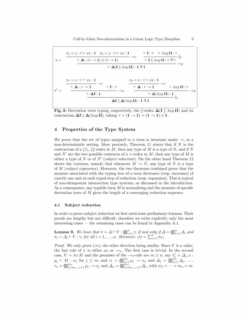
For example, let us consider the derivation tree π in Figure 3, which typesthe ‖-redex ∆(I ‖ λxy.Ω) with 1`1, and has three (E rules — one of weight 1in each subtree π1, π2, and one of weight 3 giving the conclusion, so that |π| = 5.Now, the (E-rule ending π splits into two (E-rules in the derivation tree π′

typing the contractum of ∆(I ‖ λxy.Ω), namely π′ = `∆I ‖∆(λxy.Ω) : 1`1.However, |π′| = |π|−1 since the number of the active connectives of the (E-ruleconcluding π is greater than the sum of the number of the active connectives ofits “residuals” in π′.

Finally, note that the term ∆(I ‖ λxy.Ω) reduces to the value I ‖ λy.Ω in5 = |π| steps. As we will show in Theorem 13 this does not happen by chance.


π =

π1 = x : τ ` xx : 1 π2 = x : τ ` xx : 1(I

`∆ : (τ ( 1)⊗ (τ ( 1)

` I : τ ` λxy.Ω : τ‖I

` I ‖ λxy.Ω : τ ` τ(E

`∆(I ‖ λxy.Ω) : 1 ` 1

π′ =

π1 = x : τ ` xx : 1(I

`∆ : τ ( 1 ` I : τ(E

`∆I : 1

π2 = x : τ ` xx : 1(I

`∆ : τ ( 1 ` λxy.Ω : τ(E

`∆(λxy.Ω) : 1‖I

∆I ‖∆(λxy.Ω) : 1 ` 1

Fig. 3: Derivation trees typing, respectively, the ‖-redex ∆(I ‖ λxy.Ω) and itscontractum ∆I ‖∆(λxy.Ω), taking τ = (1 ( 1) = (1 ( 1)⊗ 1.

4 Properties of the Type System

We prove that the set of types assigned to a term is invariant under →, in anon-deterministic setting. More precisely, Theorem 11 states that if N is thecontractum of a βv, ‖-redex in M , then any type of M is a type of N , and if Nand N ′ are the two possible contracta of a +-redex in M , then any type of M iseither a type of N or of N ′ (subject reduction). On the other hand Theorem 12shows the converse, namely that whenever M → N , any type of N is a typeof M (subject expansion). Moreover, the two theorems combined prove that themeasure associated with the typing tree of a term decreases (resp. increases) ofexactly one unit at each typed step of reduction (resp. expansion). This is typicalof non-idempotent intersection type systems, as discussed in the introduction.As a consequence, any typable term M is normalising and the measure of specificderivation trees of M gives the length of a converging reduction sequence.

4.1 Subject reduction

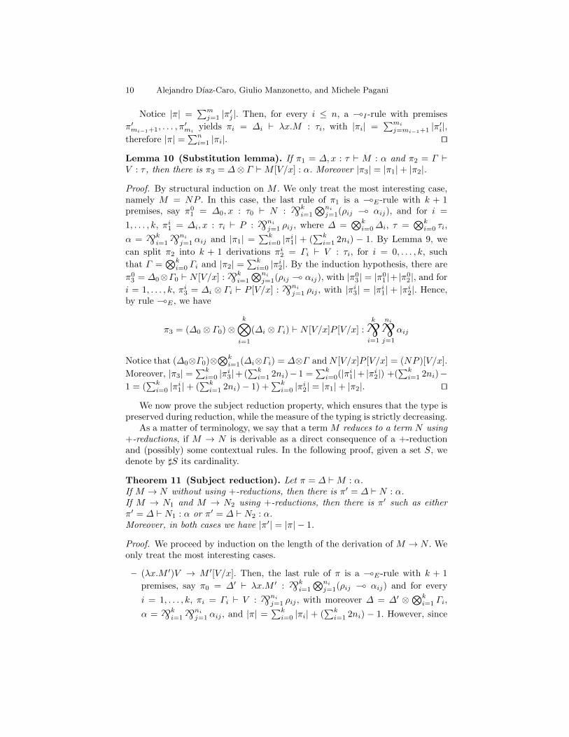
In order to prove subject reduction we first need some preliminary lemmas. Theirproofs are lengthy but not difficult, therefore we write explicitly only the mostinteresting cases — the remaining cases can be found in Appendix A.1.

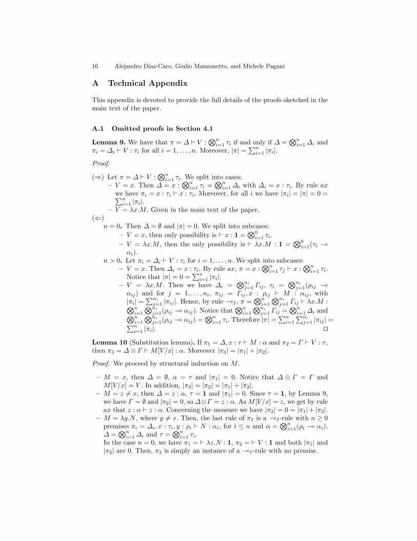
Lemma 9. We have that π = ∆ ` V :⊗n

i=1 τi if and only if ∆ =⊗n

i=1∆i andπi = ∆i ` V : τi for all i = 1, . . . , n. Moreover, |π| =

∑ni=1 |πi|.

Proof. We only prove (⇒), the other direction being similar. Since V is a value,the last rule of π is either ax or (I . The first case is trivial. In the secondcase, V = λx.M and the premises of the (I -rule are m ≥ n, say π′j = ∆j , x :

ρj ` M : αj for j ≤ m, and τ1 =⊗m1

j=1 ρj ( αj and ∆1 =⊗m1

j=1∆j , . . . ,

τn =⊗mn

j=mn−1+1 ρj ( αj and ∆n =⊗mn

j=mn−1+1∆j , with m1 + · · ·+mn = m.


Notice |π| =∑m

j=1 |π′j |. Then, for every i ≤ n, a (I -rule with premises

π′mi−1+1, . . . , π′mi

yields πi = ∆i ` λx.M : τi, with |πi| =∑mi

j=mi−1+1 |π′i|,therefore |π| =

∑ni=1 |πi|. ut

Lemma 10 (Substitution lemma). If π1 = ∆,x : τ ` M : α and π2 = Γ `V : τ , then there is π3 = ∆⊗ Γ `M [V/x] : α. Moreover |π3| = |π1|+ |π2|.

Proof. By structural induction on M . We only treat the most interesting case,namely M = NP . In this case, the last rule of π1 is a (E-rule with k + 1premises, say π0

1 = ∆0, x : τ0 ` N :˙k

i=1

⊗ni

j=1(ρij ( αij), and for i =

1, . . . , k, πi1 = ∆i, x : τi ` P :

˙ni

j=1 ρij , where ∆ =⊗k

i=0∆i, τ =⊗k

i=0 τi,

α =˙k

i=1

˙ni

j=1 αij and |π1| =∑k

i=0 |πi1| + (

∑ki=1 2ni) − 1. By Lemma 9, we

can split π2 into k + 1 derivations πi2 = Γi ` V : τi, for i = 0, . . . , k, such

that Γ =⊗k

i=0 Γi and |π2| =∑k

i=0 |πi2|. By the induction hypothesis, there are

π03 = ∆0⊗Γ0 ` N [V/x] :

˙ki=1

⊗ni

j=1(ρij ( αij), with |π03 | = |π0

1 |+ |π02 |, and for

i = 1, . . . , k, πi3 = ∆i ⊗ Γi ` P [V/x] :

˙ni

j=1 ρij , with |πi3| = |πi

1| + |πi2|. Hence,

by rule (E , we have

π3 = (∆0 ⊗ Γ0)⊗k⊗

i=1

(∆i ⊗ Γi) ` N [V/x]P [V/x] :k

i=1

ni

j=1

αij

Notice that (∆0⊗Γ0)⊗⊗k

i=1(∆i⊗Γi) = ∆⊗Γ and N [V/x]P [V/x] = (NP )[V/x].

Moreover, |π3| =∑k

i=0 |πi3|+ (

∑ki=1 2ni)− 1 =

∑ki=0(|πi

1|+ |πi2|) +(

∑ki=1 2ni)−

1 = (∑k

i=0 |πi1|+ (

∑ki=1 2ni)− 1) +

∑ki=0 |πi

2| = |π1|+ |π2|. ut

We now prove the subject reduction property, which ensures that the type ispreserved during reduction, while the measure of the typing is strictly decreasing.

As a matter of terminology, we say that a term M reduces to a term N using+-reductions, if M → N is derivable as a direct consequence of a +-reductionand (possibly) some contextual rules. In the following proof, given a set S, wedenote by ]S its cardinality.

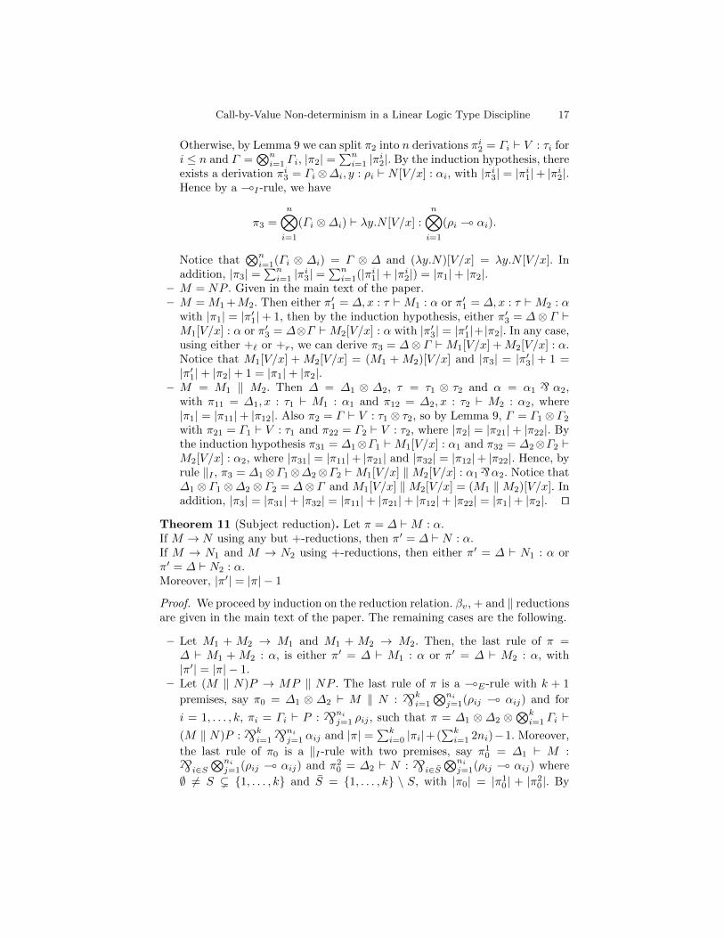
Theorem 11 (Subject reduction). Let π = ∆ `M : α.If M → N without using +-reductions, then there is π′ = ∆ ` N : α.If M → N1 and M → N2 using +-reductions, then there is π′ such as eitherπ′ = ∆ ` N1 : α or π′ = ∆ ` N2 : α.Moreover, in both cases we have |π′| = |π| − 1.

Proof. We proceed by induction on the length of the derivation of M → N . Weonly treat the most interesting cases.

– (λx.M ′)V → M ′[V/x]. Then, the last rule of π is a (E-rule with k + 1

premises, say π0 = ∆′ ` λx.M ′ :˙k

i=1

⊗ni

j=1(ρij ( αij) and for every

i = 1, . . . , k, πi = Γi ` V :˙ni

j=1 ρij , with moreover ∆ = ∆′ ⊗⊗k

i=1 Γi,

α =˙k

i=1

˙ni

j=1 αij , and |π| =∑k

i=0 |πi| + (∑k

i=1 2ni) − 1. However, since


Lemma 6 entails that k = n1 = 1 we get |π| = |π0| + |π1| + 1. In addition,the only possibility for π0 is to come from π′0 = ∆′, x : ρ ` M ′ : α, where|π0| = |π′0|. By Lemma 10, π′ = ∆′ ⊗ Γ ` M ′[V/x] : α, where |π′| =|π′0|+ |π1| = |π0|+ |π1| = |π| − 1. We conclude since ∆′ ⊗ Γ = ∆.

– Let V (M ‖ N) → VM ‖ V N . Then π = ∆ ⊗⊗k

i=1 Γi ` V (M ‖ N) :˙ki=1

˙ni

j=1 αij ends in a (E rule having as premises π0 = ∆ ` V :˙ki=1

⊗ni

j=1(ρij ( αij) and, for i = 1, . . . , k, πi = Γj ` M ‖ N :˙ni

j=1 ρij .

Thus, we have |π| =∑k

j=0 |πi|+(∑k

i=1 2ni)−1. However, by Lemma 6, k = 1,so we omit the index i where it is not needed, and |π| = |π0|+ |π1|+ 2n− 1.Then π1

1 = Γ1 ` M :˙

j∈S ρj and π21 = Γ2 ` N :

˙j∈S ρj , where

Γ = Γ1⊗Γ2, ∅ 6= S ( 1, . . . , k and S = 1, . . . , k\S with |π1| = |π11 |+|π2

1 |.By Lemma 9, we can split π0 into two derivations, πS

0 =⊗

j∈S ∆j ` V :⊗j∈S(ρj ( αj) and πS

0 =⊗

j∈S ∆j ` V :⊗

j∈S(ρj ( αj), with |πS0 | +

|πS0 | = |π0|. By rule (E , we have π1 =

⊗j∈S ∆j ⊗Γ1 ` VM :

˙j∈S αj and

π2 =⊗

j∈S ∆j⊗Γ2 ` V N :˙

j∈S αj , where |π1| = |πS0 |+ |π1

1 |+2]S−1, and

|π2| = |πS0 | + |π2

1 | + 2]S − 1. By rule ‖I , π′ =⊗n

j=1∆i ⊗ Γ1 ⊗ Γ2 ` VM ‖V N :

˙nj=1 αj , where |π′| = |π1| + |π2| = (|πS

0 | + |π11 | + 2]S − 1) + (|πS

0 | +|π2

1 |+2]S−1) = |π0|+ |π1|+2]S+2]S−2 = |π0|+ |π1|+2n−2 = |π|−1. ut

4.2 Subject Expansion

The proof of the fact that our system enjoys subject expansion follows bystraightforward induction, once one has proved the commutation of abstractionwith abstraction, application, non-deterministic choice and parallel composition.

We refer to Appendix A.2 for a detailed proof.

Theorem 12 (Subject expansion). If M → N and π = ∆ ` N : α, thenthere is π′ = ∆ `M : α, such that |π′| = |π|+ 1.

Proof. By induction on the length of the derivation of M → N , splitting intocases depending on its last rule. We only consider the most interesting case,i.e. (λx.M ′)V → M ′[V/x] where M ′ = PQ. One first needs to establish, byinduction on π, a claim about the commutation of abstraction with application.

Claim. If π = ∆ ` ((λx.P )V )((λx.Q)V ) : α, where the last rule of π is a (E

rule having k + 1 premises, then there exists π′ = ∆ ` (λx.PQ)V : α such that|π′| = |π| − k.

By definition we have N = (PQ)[V/x] = P [V/x]Q[V/x]. So, π = ∆ ` N : α

ends in a (E-rule with k+1 premises π0 = ∆′ ` P [V/x] :˙k

i=1

⊗ni

j=1 (τij ( αij)

and πi = Γi ` Q[V/x] :˙ni

j=1 τij for i = 1, . . . , k, with ∆ = ∆′ ⊗⊗k

i=1 Γi,

α =˙k

i=1

˙ni

j=1 αij and |π| =∑k

i=0 πi + (∑k

i=1 2ni) − 1. Then, by the in-

duction hypothesis, we get π′0 = ∆′ ` (λx.P )V :˙k

i=1

⊗ni

j=1(τij ( αij),

and π′i = Γi ` (λx.Q)V :˙ni

j=1 τij , with |π′i| = |πi| + 1. Hence by rule (E


we obtain π′′ = ∆′ ⊗⊗k

i=1 Γi ` ((λx.P )V )((λx.Q)V ) :˙k

i=1

˙ni

j=1 αij , with

|π′′| =∑k

i=0 |π′i|+(∑k

i=1 2ni)−1. By the above claim, we get π′ = ∆′⊗⊗k

i=1 Γi `(λx.PQ)V :

˙ki=1

˙ni

j=1 αij such that |π′| = |π′′| − k = |π|+ 1. ut

4.3 Convergence

From our “quantitative” versions of subject reduction and subject expansionone easily obtains that our type system captures exactly the weakly normalisingterms, and that the size |π| of a derivation tree π = ` M : α decreases alongthe reduction of M . However, when α satisfies in addition a suitable minimalitycondition (namely the fact that α is of shape 1` · · ·` 1), then we can be moreprecise and say that there exists a reduction from M to a normal form, havinglength exactly |π|.

In the following `k1, with k > 0, stands for 1 ` · · ·` 1 (k times).

Theorem 13. Let M be a closed term, and k > 0. There is a typing tree π for` M : `k1 iff there are values V1, . . . , Vk and a reduction M →∗ V1 ‖ · · · ‖ Vkof length |π|.

Proof. (⇒) Suppose π = ` M : `k1. We proceed by induction on |π|. IfM = V1 ‖ · · · ‖ Vk′ , then π must start with a tree of k′ − 1 rules ‖, and then k′

rules (I with conclusion, respectively, ` V1 : 1, . . . , ` Vk′ : 1. We then havek = k′, and M trivially converges to V1 ‖ · · · ‖ Vk′ in |π| = 0 steps.

Otherwise, since M is closed, there exists N such that M → N . By The-orem 11, such an N can be chosen in such a way π′ = ` N : `k1, with|π′| = |π| − 1. From the induction hypothesis we know that N converges in|π′| steps to V1 ‖ · · · ‖ Vk. Therefore, M converges in |π′| + 1 = |π| steps toV1 ‖ · · · ‖ Vk.

(⇐) Suppose that M →∗ V1 ‖ · · · ‖ Vk. By Remark 5, there is π = ` V1 ‖· · · ‖ Vk : `k1 and |π| = 0. Therefore, by the subject expansion (Theorem 12)there is π′ = ` M : `k1 and |π′| is equal to the length of the reduction M →∗V1 ‖ · · · ‖ Vk. ut

Corollary 14. Let M be closed, then M is typable if and only if M converges.

5 Adequacy and (Lack of) Full Abstraction

The choice of presenting a model through a type discipline or a reflexive objectis more a matter of taste rather than a technical decision. (Compare for instancethe type system of [18] and the interpretation of [8]). The model V associatedwith our type system lives in the category Rel of sets and relations (refer to [7]for more details) and is defined by V =

⋃n∈N Vn, with

V0 = ∅, Vn+1 =Mf(Vn)×Mf(Mf(Vn)),

where Mf(X) denotes the set of finite multisets over a set X. In fact, Mf(X)interprets in Rel the exponentials !X and ?X, whilst the cartesian product is


the linear implication (, so that V is the minimal solution of the equation V '!V ( ?!V. Recalling Equation 1 in the introduction, this means that the objectV represents “value types”, while computational types C will be represented byelements of C = !V = Mf(V) and parallel-types T as elements of T = ?C =Mf(C). This intuition can be formalized by defining two injections (·) : T→ Tand (·)• : C→ C by mutual induction, as follows: τ = [τ•], (α` β) = α ] β,1• = [], (τ ⊗ ρ)• = τ• ] ρ• and (τ ( α)• = [(τ•, α)].

It is beyond the scope of the present paper to give the explicit inductivedefinition of the interpretation of terms. For our purpose it is enough to knowthat such an interpretation can be characterised (up to isomorphism) as follows.

Definition 15. The interpretation of a closed term M is defined by [M ] = α |`M : α ⊆ T.

The interpretations of terms are naturally ordered by set-theoretical inclu-sion; an interesting problem is to determine whether there is a relationship be-tween this ordering and the following observational preorder on terms.

Definition 16 (Observational preorder). Let M,N ∈ Λ+‖ be closed. We set

M v N iff for all closed terms ~P , M ~P converges implies that N ~P converges.

A model is called adequate if [M ] ⊆ [N ] entails M v N ; it is called fullyabstract if in addition the converse holds.

The adequacy of the model V follows easily from Theorem 13 and the mono-tonicity of the interpretation.

Corollary 17 (Adequacy). For all M,N closed, if [M ] ⊆ [N ] then M v N .

On the contrary, V is not fully abstract. This is due to the fact that the call-by-value λ-calculus admits the creation of an ‘ogre’ that is able to ‘eat’ any finitesequence of arguments and converge, constituting then a top of the call-by-valueobservational preorder. Following [13], we define the ogre as Y? = ∆?∆? where∆? = λxy.xx. The ogre Y? converges since Y? → λy.Y? and remains convergentwhen applied to every sequence of values, by discarding them one at time.

Lemma 18. For all closed terms M we have M v Y?.

Proof. Given a term M and a sequence ~P = P1 · · ·Pk of closed terms it is easyto check that M ~P can converge only when ~P converges. In that case we haveY? ~P →∗ (λy.Y?)(V1 ‖ · · · ‖ Vn)P2 · · ·Pk →∗ Y?P2 · · ·Pk ‖ · · · ‖ Y?P2 · · ·Pk →∗λy.Y? ‖ · · · ‖ λy.Y?. Therefore Y? is maximal with respect to v. ut

On the other hand, we have the following characterisation of [Y?].

Lemma 19. α ∈ [Y?] iff α =⊗n

i=0(1 ( αi) with n ≥ 0 and αi ∈ [Y?] for alli ≤ n. In particular, we have that [I] 6⊆ [Y?].


Proof. The crucial point is to remark that Y? → λy.Y?, so by Theorem 11 and 12,we get [Y?] = [λy.Y?]. Therefore we have the following chain of equivalences:

α ∈ [Y?] iff α ∈ [λy.Y?]

iff α = ⊗ni=0(τi ( αi) ∈ [λy.Y?] by Lemma 6, n ≥ 0

iff α = ⊗ni=0(τi ( αi) and ∀i, τi ( αi ∈ [λy.Y?] by Lemma 9

iff α = ⊗ni=0(τi ( αi) and ∀i, τi = 1 and αi ∈ [Y?] since y /∈ FV(Y?).

We have that [I] 6⊆ [Y?] as, for instance, (1 ( 1) ( (1 ( 1) ∈ [I] \ [Y?]. ut

Summing up, get that I v Y?, while [I] 6⊆ [Y?].

6 Conclusion and future work

We introduced a call-by-value non-deterministic λ-calculus with a type systemensuring convergence. We proved that such a type system gives a bound on thelength of the lazy call-by-value reduction sequences, which is the exact lengthwhen the typing is minimal. Finally, we show that the relational model V cap-turing our type system is adequate, but not fully abstract.

As our counterexample to full abstraction contains no non-deterministic op-erators, it also holds for the standard call-by-value λ-calculus and the relationalmodel described in [7]. This is a notable difference with the call-by-name case,where the relational model is proven to be fully abstract for the pure call-by-nameλ-calculus [19], while other counterexamples (see [8, 20]) break full abstractionin presence of may or must non-deterministic operators. An open problem is tofind a relational model fully abstract for the call-by-value λ-calculus.

Various fully abstract models of may and must non-determinism are known inthe setting of Scott domain based semantics and idempotent intersection types.In particular, for the call-by-value case we mention [13, 14]. Comparing thesemodels and type systems with the ones issued from the relational semantics is aresearch direction started in [7] with some notable results. It would be interestingto reach a better understanding of the role played by intersection idempotencyin the question of full abstraction.

Another axis of research is to generalize our approach to study the conver-gence in (call-by-name and call-by-value) λ-calculi with richer algebraic struc-tures than simply may/must non-deterministic operators, such as [21, 17]. Inthese calculi the choice operator is enriched with a weight, i.e. sums of terms areof the form α.M + β.N , where α, β are scalars from a given semiring, ponder-ing the choice. We would like to design type systems characterizing convergenceproperties in these systems. First steps have been done in [22, 23].

Acknowledgements. We wish to thank Thomas Ehrhard and Simona RonchiDella Rocca for interesting discussions.


References

1. Coppo, M., Dezani-Ciancaglini, M.: A new type-assignment for λ-terms. Archivfur Math. Logik 19 (1978) 139–156

2. Salle, P.: Une generalisation de la theorie de types en λ-calcul. RAIRO: Informa-tique Theorique 14(2) (1980) 143–167

3. Krivine, J.L.: Lambda-calcul: types et modeles. Etudes et recherches en informa-tique. Masson (1990)

4. Amadio, R., Curien, P.L.: Domains and Lambda-Calculi. Number 46 in CambridgeTracts in Theoretical Computer Science. Cambridge University Press (1998)

5. de Carvalho, D.: Execution time of lambda-terms via denotational semantics andintersection types. To appear in Math. Struct. in Comp. Sci. (2008)

6. Bernadet, A., Lengrand, S.: Complexity of strongly normalising λ-terms via non-idempotent intersection types. In: FOSSACS 2011. (2011) 88–107

7. Ehrhard, T.: Collapsing non-idempotent intersection types. In: CSL’12. Volume 16of LIPIcs. (2012) 259–273

8. Bucciarelli, A., Ehrhard, T., Manzonetto, G.: A relational semantics for parallelismand non-determinism in a functional setting. APAL 163(7) (2012) 918–934

9. Girard, J.Y.: Linear logic. Theoretical Computer Science 50 (1987) 1–10210. Maraist, J., Odersky, M., Turner, D.N., Wadler, P.: Call-by-name, call-by-value,

call-by-need and the linear λ-calculus. Theor. Comp. Sci. 228(1-2) (1999) 175–21011. Laurent, O.: Etude de la polarisation en logique. PhD thesis, Universite de Aix-

Marseille II, France (2002)12. Dezani-Ciancaglini, M., de’Liguoro, U., Piperno, A.: Filter models for conjunctive-

disjunctive lambda-calculi. Theor. Comp. Sci. 170(1-2) (1996) 83–12813. Boudol, G.: Lambda-calculi for (strict) parallel functions. Information and Com-

putation 108(1) (1994) 51–12714. Dezani-Ciancaglini, M., de’Liguoro, U., Piperno, A.: A filter model for concurrent

lambda-calculus. SIAM J. Comput. 27(5) (1998) 1376–141915. Plotkin, G.D.: Call-by-name, call-by-value and the λ-calculus. Theor. Comp. Sci.

1(2) (1975) 125–15916. Barendregt, H.: The lambda calculus: its syntax and semantics. North-Holland,

Amsterdam (1984)17. Arrighi, P., Dowek, G.: Linear-algebraic lambda-calculus: higher-order, encodings,

and confluence. In: RTA’08. Volume 5117 of LNCS., Springer (2008) 17–3118. Pagani, M., Ronchi Della Rocca, S.: Linearity, non-determinism and solvability.

Fundam. Inform. 103(1-4) (2010) 173–20219. Manzonetto, G.: A general class of models of H?. In: MFCS’09. Volume 5734 of

LNCS., Springer (2009) 574–58620. Breuvart, F.: On the discriminating power of tests in the resource λ-calculus

Submitted. Draft available at http://hal.archives-ouvertes.fr/hal-00698609.21. Vaux, L.: The algebraic lambda calculus. Math. Struct. in Comp. Sci. 19(5) (2009)

1029–105922. Arrighi, P., Dıaz-Caro, A.: A System F accounting for scalars. Logical Methods

in Computer Science 8(1) (2012)23. Arrighi, P., Dıaz-Caro, A., Valiron, B.: A type system for the vectorial aspects of

the linear-algebraic λ-calculus. In: DCM’11. Volume 88 of EPTCS. (2012) 1–15


A Technical Appendix

This appendix is devoted to provide the full details of the proofs sketched in themain text of the paper.

A.1 Omitted proofs in Section 4.1

Lemma 9. We have that π = ∆ ` V :⊗n

i=1 τi if and only if ∆ =⊗n

i=1∆i andπi = ∆i ` V : τi for all i = 1, . . . , n. Moreover, |π| =

∑ni=1 |πi|.

Proof.

(⇒) Let π = ∆ ` V :⊗n

i=1 τi. We split into cases:– V = x. Then ∆ = x :

⊗ni=1 τi =

⊗ni=1∆i with ∆i = x : τi. By rule ax

we have πi = x : τi ` x : τi. Moreover, for all i we have |πi| = |π| = 0 =∑ni=1 |πi|.

– V = λx.M . Given in the main text of the paper.(⇐)

n = 0. Then ∆ = ∅ and |π| = 0. We split into subcases:

– V = x, then only possibility is ` x : 1 =⊗0

i=1 τi.

– V = λx.M , then the only possibility is ` λx.M : 1 =⊗0

i=1(τi (αi).

n > 0. Let πi = ∆i ` V : τi for i = 1, . . . , n. We split into subcases:– V = x. Then ∆i = x : τi. By rule ax, π = x :

⊗ni=1 τj ` x :

⊗ni=1 τi.

Notice that |π| = 0 =∑n

i=1 |πi|.– V = λx.M . Then we have ∆i =

⊗ni

j=1 Γij , τi =⊗ni

j=1(ρij (αij) and for j = 1, . . . , ni, πij = Γij , x : ρij ` M : αij , with|πi| =

∑ni

j=1 |πij |. Hence, by rule (I , π =⊗n

i=1

⊗ni

j=1 Γij ` λx.M :⊗ni=1

⊗ni

j=1(ρij ( αij). Notice that⊗n

i=1

⊗ni

j=1 Γij =⊗n

i=1∆i and⊗ni=1

⊗ni

j=1(ρij ( αij) =⊗n

i=1 τi. Therefore |π| =∑n

i=1

∑ni

j=1 |πij | =∑ni=1 |πi|. ut

Lemma 10 (Substitution lemma). If π1 = ∆,x : τ `M : α and π2 = Γ ` V : τ ,then π3 = ∆⊗ Γ `M [V/x] : α. Moreover |π3| = |π1|+ |π2|.

Proof. We proceed by structural induction on M .

– M = x, then ∆ = ∅, α = τ and |π1| = 0. Notice that ∆ ⊗ Γ = Γ andM [V/x] = V . In addition, |π3| = |π2| = |π1|+ |π2|.

– M = z 6= x, then ∆ = z : α, τ = 1 and |π1| = 0. Since τ = 1, by Lemma 9,we have Γ = ∅ and |π2| = 0, so ∆⊗Γ = z : α. As M [V/x] = z, we get by ruleax that z : α ` z : α. Concerning the measure we have |π3| = 0 = |π1|+ |π2|.

– M = λy.N , where y 6= x. Then, the last rule of π1 is a (I -rule with n ≥ 0premises πi = ∆i, x : τi, y : ρi ` N : αi, for i ≤ n and α =

⊗ni=1(ρi ( αi),

∆ =⊗n

i=1∆i and τ =⊗n

i=1 τi.In the case n = 0, we have π1 = ` λz.N : 1, π2 = ` V : 1 and both |π1| and|π2| are 0. Then, π3 is simply an instance of a (I -rule with no premise.


Otherwise, by Lemma 9 we can split π2 into n derivations πi2 = Γi ` V : τi for

i ≤ n and Γ =⊗n

i=1 Γi, |π2| =∑n

i=1 |πi2|. By the induction hypothesis, there

exists a derivation πi3 = Γi⊗∆i, y : ρi ` N [V/x] : αi, with |πi

3| = |πi1|+ |πi

2|.Hence by a (I -rule, we have

π3 =

n⊗i=1

(Γi ⊗∆i) ` λy.N [V/x] :

n⊗i=1

(ρi ( αi).

Notice that⊗n

i=1(Γi ⊗ ∆i) = Γ ⊗ ∆ and (λy.N)[V/x] = λy.N [V/x]. Inaddition, |π3| =

∑ni=1 |πi

3| =∑n

i=1(|πi1|+ |πi

2|) = |π1|+ |π2|.– M = NP . Given in the main text of the paper.– M = M1 +M2. Then either π′1 = ∆,x : τ `M1 : α or π′1 = ∆,x : τ `M2 : α

with |π1| = |π′1|+ 1, then by the induction hypothesis, either π′3 = ∆⊗ Γ `M1[V/x] : α or π′3 = ∆⊗Γ `M2[V/x] : α with |π′3| = |π′1|+ |π2|. In any case,using either +` or +r, we can derive π3 = ∆⊗ Γ `M1[V/x] +M2[V/x] : α.Notice that M1[V/x] + M2[V/x] = (M1 + M2)[V/x] and |π3| = |π′3| + 1 =|π′1|+ |π2|+ 1 = |π1|+ |π2|.

– M = M1 ‖ M2. Then ∆ = ∆1 ⊗ ∆2, τ = τ1 ⊗ τ2 and α = α1 ` α2,with π11 = ∆1, x : τ1 ` M1 : α1 and π12 = ∆2, x : τ2 ` M2 : α2, where|π1| = |π11|+ |π12|. Also π2 = Γ ` V : τ1 ⊗ τ2, so by Lemma 9, Γ = Γ1 ⊗ Γ2

with π21 = Γ1 ` V : τ1 and π22 = Γ2 ` V : τ2, where |π2| = |π21|+ |π22|. Bythe induction hypothesis π31 = ∆1⊗Γ1 `M1[V/x] : α1 and π32 = ∆2⊗Γ2 `M2[V/x] : α2, where |π31| = |π11|+ |π21| and |π32| = |π12|+ |π22|. Hence, byrule ‖I , π3 = ∆1⊗Γ1⊗∆2⊗Γ2 `M1[V/x] ‖M2[V/x] : α1 `α2. Notice that∆1 ⊗ Γ1 ⊗∆2 ⊗ Γ2 = ∆⊗ Γ and M1[V/x] ‖M2[V/x] = (M1 ‖M2)[V/x]. Inaddition, |π3| = |π31|+ |π32| = |π11|+ |π21|+ |π12|+ |π22| = |π1|+ |π2|. ut

Theorem 11 (Subject reduction). Let π = ∆ `M : α.If M → N using any but +-reductions, then π′ = ∆ ` N : α.If M → N1 and M → N2 using +-reductions, then either π′ = ∆ ` N1 : α orπ′ = ∆ ` N2 : α.Moreover, |π′| = |π| − 1

Proof. We proceed by induction on the reduction relation. βv, + and ‖ reductionsare given in the main text of the paper. The remaining cases are the following.

– Let M1 + M2 → M1 and M1 + M2 → M2. Then, the last rule of π =∆ ` M1 + M2 : α, is either π′ = ∆ ` M1 : α or π′ = ∆ ` M2 : α, with|π′| = |π| − 1.

– Let (M ‖ N)P → MP ‖ NP . The last rule of π is a (E-rule with k + 1

premises, say π0 = ∆1 ⊗ ∆2 ` M ‖ N :˙k

i=1

⊗ni

j=1(ρij ( αij) and for

i = 1, . . . , k, πi = Γi ` P :˙ni

j=1 ρij , such that π = ∆1 ⊗ ∆2 ⊗⊗k

i=1 Γi `(M ‖ N)P :

˙ki=1

˙ni

j=1 αij and |π| =∑k

i=0 |πi|+(∑k

i=1 2ni)−1. Moreover,

the last rule of π0 is a ‖I -rule with two premises, say π10 = ∆1 ` M :˙

i∈S⊗ni

j=1(ρij ( αij) and π20 = ∆2 ` N :

˙i∈S

⊗ni

j=1(ρij ( αij) where

∅ 6= S ( 1, . . . , k and S = 1, . . . , k \ S, with |π0| = |π10 | + |π2

0 |. By


rule (E , we have π1 = ∆1 ⊗⊗

i∈S Γi ` MP :˙

i∈S˙ni

j=1 αij and π2 =

∆2 ⊗⊗

i∈S Γi ` NP :˙

i∈S˙ni

j=1 αij , where |π1| = |π10 | +

∑i∈S |πi| +

(∑

i∈S 2ni) − 1 and |π2| = |π20 | +

∑i∈S |πi| + (

∑i∈S 2ni) − 1. Then by rule

‖I , π′ = ∆1⊗∆2⊗⊗k

i=1 Γi `MP ‖ NP :˙k

i=1

˙ni

j=1 αij , with |π′| = |π1|+|π2| = |π1

0 |+∑

i∈S |πi|+(∑

i∈S 2ni)−1+ |π20 |+

∑i∈S |πi|+(

∑i∈S 2ni)−1 =∑k

i=0 |πi|+ (∑k

i=1 2ni)− 2 = |π| − 1.

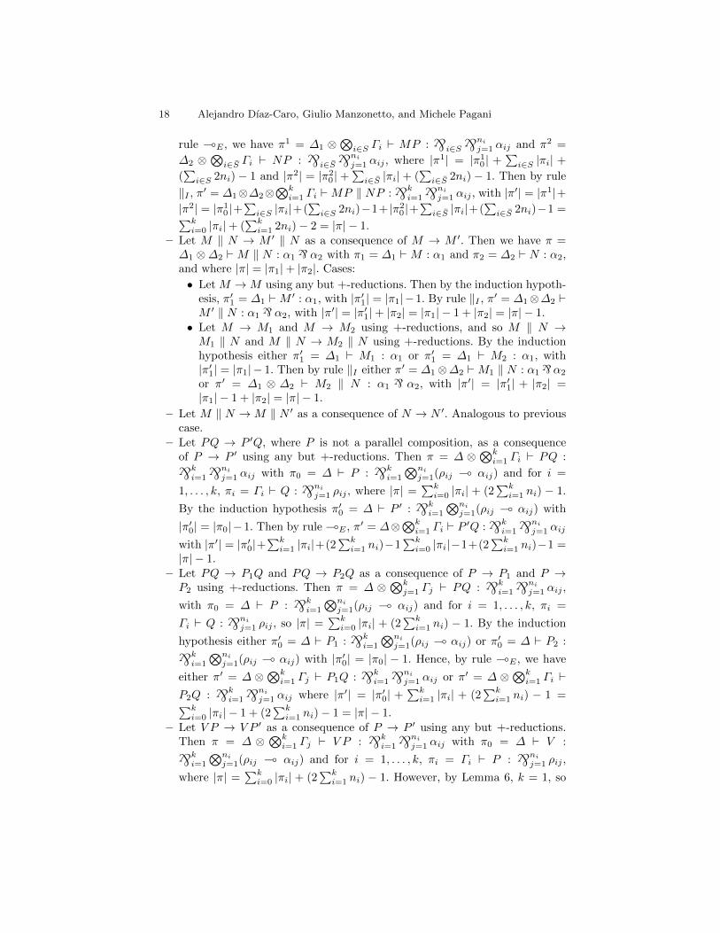
– Let M ‖ N → M ′ ‖ N as a consequence of M → M ′. Then we have π =∆1 ⊗∆2 `M ‖ N : α1 ` α2 with π1 = ∆1 `M : α1 and π2 = ∆2 ` N : α2,and where |π| = |π1|+ |π2|. Cases:

• Let M →M using any but +-reductions. Then by the induction hypoth-esis, π′1 = ∆1 `M ′ : α1, with |π′1| = |π1|−1. By rule ‖I , π′ = ∆1⊗∆2 `M ′ ‖ N : α1 ` α2, with |π′| = |π′1|+ |π2| = |π1| − 1 + |π2| = |π| − 1.

• Let M → M1 and M → M2 using +-reductions, and so M ‖ N →M1 ‖ N and M ‖ N → M2 ‖ N using +-reductions. By the inductionhypothesis either π′1 = ∆1 ` M1 : α1 or π′1 = ∆1 ` M2 : α1, with|π′1| = |π1| − 1. Then by rule ‖I either π′ = ∆1⊗∆2 `M1 ‖ N : α1 `α2

or π′ = ∆1 ⊗ ∆2 ` M2 ‖ N : α1 ` α2, with |π′| = |π′1| + |π2| =|π1| − 1 + |π2| = |π| − 1.

– Let M ‖ N →M ‖ N ′ as a consequence of N → N ′. Analogous to previouscase.

– Let PQ → P ′Q, where P is not a parallel composition, as a consequenceof P → P ′ using any but +-reductions. Then π = ∆ ⊗

⊗ki=1 Γi ` PQ :˙k

i=1

˙ni

j=1 αij with π0 = ∆ ` P :˙k

i=1

⊗ni

j=1(ρij ( αij) and for i =

1, . . . , k, πi = Γi ` Q :˙ni

j=1 ρij , where |π| =∑k

i=0 |πi| + (2∑k

i=1 ni) − 1.

By the induction hypothesis π′0 = ∆ ` P ′ :˙k

i=1

⊗ni

j=1(ρij ( αij) with

|π′0| = |π0|−1. Then by rule (E , π′ = ∆⊗⊗k

i=1 Γi ` P ′Q :˙k

i=1

˙ni

j=1 αij

with |π′| = |π′0|+∑k

i=1 |πi|+(2∑k

i=1 ni)−1∑k

i=0 |πi|−1+(2∑k

i=1 ni)−1 =|π| − 1.

– Let PQ → P1Q and PQ → P2Q as a consequence of P → P1 and P →P2 using +-reductions. Then π = ∆ ⊗

⊗kj=1 Γj ` PQ :

˙ki=1

˙ni

j=1 αij ,

with π0 = ∆ ` P :˙k

i=1

⊗ni

j=1(ρij ( αij) and for i = 1, . . . , k, πi =

Γi ` Q :˙ni

j=1 ρij , so |π| =∑k

i=0 |πi| + (2∑k

i=1 ni) − 1. By the induction

hypothesis either π′0 = ∆ ` P1 :˙k

i=1

⊗ni

j=1(ρij ( αij) or π′0 = ∆ ` P2 :˙ki=1

⊗ni

j=1(ρij ( αij) with |π′0| = |π0| − 1. Hence, by rule (E , we have

either π′ = ∆ ⊗⊗k

i=1 Γj ` P1Q :˙k

i=1

˙ni

j=1 αij or π′ = ∆ ⊗⊗k

i=1 Γi `P2Q :

˙ki=1

˙ni

j=1 αij where |π′| = |π′0| +∑k

i=1 |πi| + (2∑k

i=1 ni) − 1 =∑ki=0 |πi| − 1 + (2

∑ki=1 ni)− 1 = |π| − 1.

– Let V P → V P ′ as a consequence of P → P ′ using any but +-reductions.Then π = ∆ ⊗

⊗ki=1 Γj ` V P :

˙ki=1

˙ni

j=1 αij with π0 = ∆ ` V :˙ki=1

⊗ni

j=1(ρij ( αij) and for i = 1, . . . , k, πi = Γi ` P :˙ni

j=1 ρij ,

where |π| =∑k

i=0 |πi| + (2∑k

i=1 ni) − 1. However, by Lemma 6, k = 1, so


we omit the index i when not needed, and |π| = |π0|+ |π1|+ 2n− 1. By theinduction hypothesis, π′1 = Γ ` P ′ :

˙nj=1 ρj , with |π′1| = |π1| − 1. Then by

rule (E , π′ = ∆ ⊗ Γ ` V P ′ :˙n

j=1 αj where |π′| = |π0| + |π′1| + 2n − 1 =|π0|+ |π1| − 1 + 2n− 1 = |π| − 1.

– Let V P → V P1 and V P → V P2 as a consequence of P → P1 and P → P2

using +-reductions. Then π = ∆ ⊗⊗k

i=1 Γi ` V P :˙k

i=1

˙ni

j=1 αij , with

π0 = ∆ ` V :˙k

i=1

⊗ni

j=1(ρij ( αij) and for i = 1, . . . , k πi = Γi `P :

˙ni

j=1 ρij . So, |π| =∑k

i=0 |πi|+ (2∑k

i=1 ni)− 1. However, by Lemma 6,k = 1, so we omit the index i when not needed, and |π| = |π0|+ |π1|+2n−1.By the induction hypothesis, either π′1 = Γ ` P1 :

˙nj=1 ρj or π′1 = Γ `

P2 :˙n

j=1 ρj , with |π′1| = |π1| − 1. Hence by rule (E , we have either

π′ = ∆ ⊗ Γ ` V P1 :˙n

j=1 αj or π′ = ∆ ⊗ Γ ` V P2 :˙n

j=1 αj , where|π′| = |π0|+ |π′1|+ 2n− 1 = |π0|+ |π1| − 1 + 2n− 1 = |π| − 1. ut

A.2 The Proof of Subject Expansion

As mentioned in Section 4.2, to prove that the subject expansion holds, wefirst need some technical lemmas stating the commutation of abstraction withabstraction, application, non-deterministic choice and parallel composition.

In the following proofs we silently use the fact that the type of a value mustbe a computational-type (Lemma 6) to simplify our derivation trees.

Lemma 20 (Abstraction commutation). If π = ∆ ` λy.(λx.M)V :⊗n

i=1(ρi (αi) and y /∈ FV(V ), then there exists π′ = ∆ ` (λx.λy.M)V :

⊗ni=1(ρi ( αi)

such that |π′| = |π| − n+ 1.

Proof. If ∆ ` λy.(λx.M)V :⊗n

i=1(ρi ( αi), then we have ∆ =⊗n

i=1(∆i ⊗ Γi),with the following π derivation (since y /∈ FV(V )):

πi = ∆i, y : τi, x : ρi `M : αi(I

∆i, y : τi ` λx.M : ρi ( αi π′i = Γi ` V : ρi(E

∆i ⊗ Γi, y : τi ` (λx.M)V : αi i = 1, . . . , n(In⊗

i=1

(∆i ⊗ Γi) ` λy.(λx.M)V :

n⊗i=1

(τi ( αi)

So |π| =∑n

i=1(|πi|+ |π′i|+ 1) =∑n

i=1 |πi|+∑n

i=1 |π′i|+ n.


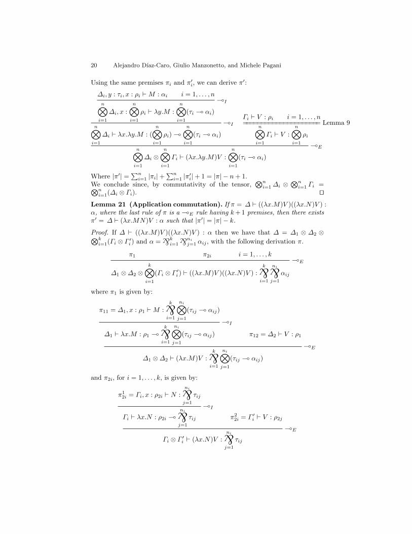
Using the same premises πi and π′i, we can derive π′:

∆i, y : τi, x : ρi `M : αi i = 1, . . . , n(In⊗

i=1

∆i, x :

n⊗i=1

ρi ` λy.M :

n⊗i=1

(τi ( αi)

(In⊗i=1

∆i ` λx.λy.M : (

n⊗i=1

ρi) (n⊗

i=1

(τi ( αi)

Γi ` V : ρi i = 1, . . . , n===================== Lemma 9

n⊗i=1

Γi ` V :

n⊗i=1

ρi

(En⊗i=1

∆i ⊗n⊗

i=1

Γi ` (λx.λy.M)V :

n⊗i=1

(τi ( αi)

Where |π′| =∑n

i=1 |πi|+∑n

i=1 |π′i|+ 1 = |π| − n+ 1.We conclude since, by commutativity of the tensor,

⊗ni=1∆i ⊗

⊗ni=1 Γi =⊗n

i=1(∆i ⊗ Γi). ut

Lemma 21 (Application commutation). If π = ∆ ` ((λx.M)V )((λx.N)V ) :α, where the last rule of π is a (E rule having k+ 1 premises, then there existsπ′ = ∆ ` (λx.MN)V : α such that |π′| = |π| − k.

Proof. If ∆ ` ((λx.M)V )((λx.N)V ) : α then we have that ∆ = ∆1 ⊗ ∆2 ⊗⊗ki=1(Γi ⊗ Γ ′i ) and α =

˙ki=1

˙ni

j=1 αij , with the following derivation π.

π1 π2i i = 1, . . . , k(E

∆1 ⊗∆2 ⊗k⊗

i=1

(Γi ⊗ Γ ′i ) ` ((λx.M)V )((λx.N)V ) :k

i=1

ni

j=1

αij

where π1 is given by:

π11 = ∆1, x : ρ1 `M :k

i=1

ni⊗j=1

(τij ( αij)

(I

∆1 ` λx.M : ρ1 (k

i=1

ni⊗j=1

(τij ( αij) π12 = ∆2 ` V : ρ1

(E

∆1 ⊗∆2 ` (λx.M)V :k

i=1

ni⊗j=1

(τij ( αij)

and π2i, for i = 1, . . . , k, is given by:

π12i = Γi, x : ρ2i ` N :

ni

j=1

τij

(I

Γi ` λx.N : ρ2i (ni

j=1

τij π22i = Γ ′i ` V : ρ2j

(E

Γi ⊗ Γ ′i ` (λx.N)V :ni

j=1

τij


So, |π| = |π1| +∑k

i=1 |π2i| + (∑k

i=1 2ni) − 1 = |π11| + |π12| + 1 +∑k

i=1(|π12i| +

|π22i|+ 1) + (

∑ki=1 2ni)− 1.

Using the same premises, we can derive, first π′1:

π11 π12i i = 1, . . . , k

(E

∆1 ⊗k⊗

i=1

Γi, x : ρ1 ⊗k⊗

i=1

ρ2i `MN :k

i=1

ni

j=1

αij

(I

∆1 ⊗k⊗

i=1

Γi ` λx.MN : (ρ1 ⊗k⊗

i=1

ρ2i) (k

i=1

ni

j=1

αij

Second, by Lemma 9, we have π′2 = ∆2 ⊗⊗k

i=1 Γ′i ` V : ρ1 ⊗

⊗ki=1 ρ2i. So, we

get:

π′ =

π′1 π′2(E

∆1 ⊗k⊗

i=1

Γi ⊗∆2 ⊗k⊗

i=1

Γ ′i ` (λx.MN)V :k

i=1

ni

j=1

αij

Hence |π′| = |π′1|+ |π′2|+ 1 = |π11|+∑k

i=1 |π12i|+ (

∑ki=1 2ni)− 1 +

∑ki=1 |π2

2i|+|π12| = |π| − k.

We conclude since ∆1⊗⊗k

i=1 Γi⊗∆2⊗⊗k

i=1 Γ′i = ∆1⊗∆2⊗

⊗ki=1(Γi⊗Γ ′i ). ut

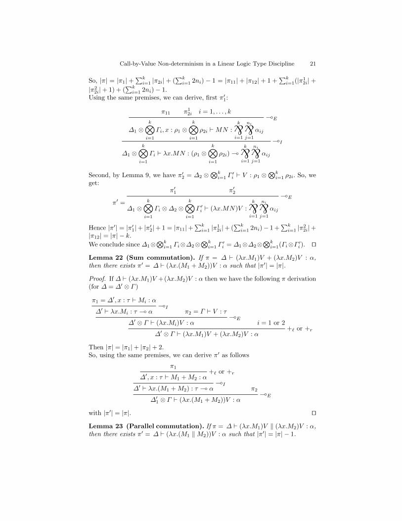
Lemma 22 (Sum commutation). If π = ∆ ` (λx.M1)V + (λx.M2)V : α,then there exists π′ = ∆ ` (λx.(M1 +M2))V : α such that |π′| = |π|.

Proof. If ∆ ` (λx.M1)V +(λx.M2)V : α then we have the following π derivation(for ∆ = ∆′ ⊗ Γ )

π1 = ∆′, x : τ `Mi : α(I

∆′ ` λx.Mi : τ ( α π2 = Γ ` V : τ(E

∆′ ⊗ Γ ` (λx.Mi)V : α i = 1 or 2+` or +r

∆′ ⊗ Γ ` (λx.M1)V + (λx.M2)V : α

Then |π| = |π1|+ |π2|+ 2.So, using the same premises, we can derive π′ as follows

π1+` or +r

∆′, x : τ `M1 +M2 : α(I

∆′ ` λx.(M1 +M2) : τ ( α π2(E

∆′1 ⊗ Γ ` (λx.(M1 +M2))V : α

with |π′| = |π|. ut

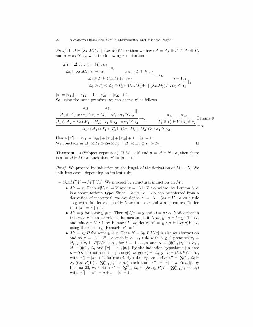
Lemma 23 (Parallel commutation). If π = ∆ ` (λx.M1)V ‖ (λx.M2)V : α,then there exists π′ = ∆ ` (λx.(M1 ‖M2))V : α such that |π′| = |π| − 1.


Proof. If ∆ ` (λx.M1)V ‖ (λx.M2)V : α then we have ∆ = ∆1 ⊗ Γ1 ⊗∆2 ⊗ Γ2

and α = α1 ` α2, with the following π derivation.

πi1 = ∆i, x : τi `Mi : αi(I

∆h ` λx.Mi : τi ( αi πi2 = Γi ` V : τi(E

∆i ⊗ Γi ` (λx.Mi)V : αi i = 1, 2‖I

∆1 ⊗ Γ1 ⊗∆2 ⊗ Γ2 ` (λx.M1)V ‖ (λx.M2)V : α1 ` α2

|π| = |π11|+ |π12|+ 1 + |π21|+ |π22|+ 1

So, using the same premises, we can derive π′ as follows

π11 π21‖I

∆1 ⊗∆2, x : τ1 ⊗ τ2 `M1 ‖M2 : α1 ` α2(I

∆1 ⊗∆2 ` λx.(M1 ‖M2) : τ1 ⊗ τ2 ( α1 ` α2

π12 π22================ Lemma 9Γ1 ⊗ Γ2 ` V : τ1 ⊗ τ2

(E∆1 ⊗∆2 ⊗ Γ1 ⊗ Γ2 ` (λx.(M1 ‖M2))V : α1 ` α2

Hence |π′| = |π11|+ |π21|+ |π12|+ |π22|+ 1 = |π| − 1.

We conclude as ∆1 ⊗ Γ1 ⊗∆2 ⊗ Γ2 = ∆1 ⊗∆2 ⊗ Γ1 ⊗ Γ2. ut

Theorem 12 (Subject expansion). If M → N and π = ∆ ` N : α, then thereis π′ = ∆ `M : α, such that |π′| = |π|+ 1.

Proof. We proceed by induction on the length of the derivation of M → N . Wesplit into cases, depending on its last rule.

– (λx.M ′)V →M ′[V/x]. We proceed by structural induction on M ′.

• M ′ = x. Then x[V/x] = V and π = ∆ ` V : α where, by Lemma 6, αis a computational-type. Since ` λx.x : α ( α can be inferred from aderivation of measure 0, we can define π′ = ∆ ` (λx.x)V : α as a rule(E with the derivation of ` λx.x : α ( α and π as premises. Noticethat |π′| = |π|+ 1.

• M ′ = y for some y 6= x. Then y[V/x] = y and ∆ = y : α. Notice that inthis case π is an ax rule, so its measure is 0. Now, y : α ` λx.y : 1 ( αand, since ` V : 1 by Remark 5, we derive π′ = y : α ` (λx.y)V : αusing the rule (E . Remark |π′| = 1.

• M ′ = λy.P for some y 6= x. Then N = λy.P [V/x] is also an abstractionand so π = ∆ ` N : α ends in a (I -rule with n ≥ 0 premises πi =∆i, y : τi ` P [V/x] : αi, for i = 1, . . . , n and α =

⊗ni=1(τi ( αi),

∆ =⊗n

i=1∆i and |π| =∑

i |πi|. By the induction hypothesis (in casen = 0 we do not need this passage), we get π′i = ∆i, y : τi ` (λx.P )V : αi,with |π′i| = |πi|+ 1, for each i. By rule (I , we derive π′′ =

⊗ni=1∆i `

λy.((λx.P )V ) :⊗n

i=1(τi ( αi), such that |π′′| = |π| + n Finally, byLemma 20, we obtain π′ =

⊗ni=1∆i ` (λx.λy.P )V :

⊗ni=1(τi ( αi)

with |π′| = |π′′| − n+ 1 = |π|+ 1.


• M ′ = PQ. By definition we have N = (PQ)[V/x] = P [V/x]Q[V/x]. So,π = ∆ ` N : α ends in a (E-rule with k + 1 premises π0 = ∆′ `P [V/x] :

˙ki=1

⊗ni

j=1(τij ( αij) and πi = Γi ` Q[V/x] :˙ni

j=1 τij

for i = 1, . . . , k, with ∆ = ∆′ ⊗⊗k

i=1 Γi, α =˙k

i=1

˙ni

j=1 αij and

|π| =∑k

i=0 πi + (∑k

i=1 2ni) − 1. Then, by the induction hypothesis,

we get π′0 = ∆′ ` (λx.P )V :˙k

i=1

⊗ni

j=1(τij ( αij), and π′i = Γi `(λx.Q)V :

˙ni

j=1 τij , with |π′i| = |πi| + 1. Hence by rule (E we obtain

π′′ = ∆′⊗⊗k

i=1 Γi ` ((λx.P )V )((λx.Q)V ) :˙k

i=1

˙ni

j=1 αij , with |π′′| =∑ki=0 |π′i|+ (

∑ki=1 2ni)− 1. By Lemma 21, we get π′ = ∆′ ⊗

⊗ki=1 Γi `

(λx.PQ)V :˙k

i=1

˙ni

j=1 αij such that |π′| = |π′′| − k = |π|+ 1.• M ′ = P +Q. Now, by definition we have N = (P +Q)[V/x] = P [V/x] +Q[V/x]. Then either π1 = ∆ ` P [V/x] : α or π1 = ∆ ` Q[V/x] : α, with|π1| = |π| − 1. Hence by the induction hypothesis, there exists eitherπ′1 = ∆ ` (λx.P )V : α or π′1 = ∆ ` (λx.Q)V : α with |π′1| = |π1| + 1.In both cases, either by rule +` or +r, we get π2 = ∆ ` (λx.P )V +(λx.Q)V : α, which entails, by Lemma 22, π′ = ∆ ` (λx.(P +Q))V : αwith |π′| = |π|+ 1.

• M ′ = P ‖ Q. By definition N = (P ‖ Q)[V/x] = P [V/x] ‖ Q[V/x], soπ = ∆ ` N : α ends in a ‖I rule with premises π1 = ∆1 ` P [V/x] : α1

and π2 = ∆2 ` Q[V/x] : α2, with ∆ = ∆1 ⊗∆2, α = α1 ` α2 and |π| =|π1|+ |π2|. By the induction hypothesis, we get π′1 = ∆1 ` (λx.P )V : α1

and π′2 = ∆2 ` (λx.Q)V : α2. Therefore, by applying the rule ‖I to π′1and π′2, we derive π3 = ∆1 ⊗∆2 ` (λx.P )V ‖ (λx.Q)V : α1 ` α2 suchthat |π3| = |π′1| + |π′2| = |π1| + 1 + |π2| + 1 = |π| + 2. From Lemma 23,we get π′ = ∆1 ⊗∆2 ` (λx.(P ‖ Q))V : α1 ` α2 with |π′| = |π|+ 1.

– P+Q→ P , with ∆ ` P : α. Then, by rule +` we get ∆ ` P+Q : α. Checkingthe measure is trivial. Symmetrically we deduce the case P +Q→ Q

– (Q1 ‖ Q2)P → Q1P ‖ Q2P . Then, π = ∆ ` N : α ends in a rule ‖Iwith two premises π1 = ∆1 ` Q1P : α1 and π2 = ∆2 ` Q2P : α2, suchthat ∆ = ∆1 ⊗ ∆2, α = α1 ` α2 and |π| = |π1| + |π2|. Moreover, the lastrule of πh, for h = 1, 2, is a (E rule with kh + 1 premises, say πh0 =Γh0 ` Qh :

˙kh

i=1

⊗nh1

j=1(τhij ( αhij), for every i = 1, . . . , kh, πhi = Γhi `P :

˙nhi

j=1 τhij , where ∆h =⊗kh

i=0 Γhi, αh =˙kh

i=1

˙nhi

j=1 αhij . Notice that

|πh| =∑kh

i=0 |πhi|+ (∑kh

i=1 2nhi)− 1.By applying the rule ‖I to π10 and π20, we get a derivation π30 = Γ10 ⊗Γ20 ` Q1 ‖ Q2 : (

˙k1

i=1

⊗n1i

j=1(τ1ij ( α1ij)) ` (˙k2

i=1

⊗n2i

j=1(τ2ij ( α2ij)).

Therefore, by rule (E , we have the derivation π′ = Γ10⊗Γ20⊗ (⊗k1

i=1 Γ1i⊗⊗k2

i=1 Γ2i) ` (Q1 ‖ Q2)P : (˙k1

i=1

˙n1i

j=1 α1ij) ` (˙k2

i=1

˙n2i

j=1 α2ij). Notice

that |π′| =∑k1

i=0 |π1i|+∑k2

i=0 |π2i|+ (∑k1

i=0 2ni +∑k2

i=0 2ni)− 1 = |π| − 1.– V (P1 ‖ P2) → V P1 ‖ V P2. Then, π = ∆ ` N : α ends in a rule ‖I with

two premises π1 = ∆1 ` V P1 : α1 and π2 = ∆2 ` V P2 : α2, such that ∆ =∆1⊗∆2, α = α1`α2 and |π| = |π1|+|π2|. As in the previous case, for h = 1, 2,πh ends is a (E rule. Since V is a value, it can have only a computational


type (Lemma 6), and so the last (E rule of πh has exactly two premises,say πh0 = Γh0 ` V :

⊗nh

j=1(τhj ( αhj) and πh1 = Γh1 ` Ph :˙nh

j=1 τhj ,

where ∆h = Γh0 ⊗ Γh1, αh =˙nh

j=1 αhj , and |πh| = |πh0|+ |πh1|+ 2nh − 1.The derivation π′ is obtained in three steps. First, we apply the rule ‖I toπ11 and π21, getting a derivation of Γ11 ⊗ Γ21 ` P1 ‖ P2 : (

˙n1

j=1 τ1j) `(˙n2

j=1 τ2j). Then, by Lemma 9, we get Γ10 ⊗ Γ20 ` V : (⊗n1

j=1(τ1j (α1j))⊗ (

⊗n2

j=1(τ2j ( α2j)). Finally, we achieve π′ by applying a rule (E tothe previous two. Notice that |π′| = |π10|+|π20|+|π11|+|π22|+2(n1+n2)−1 =|π|+ 1.

– P ‖ Q → P ′ ‖ Q as a consequence of P → P ′. Then, ∆ = ∆1 ⊗ ∆2 andα = α1 ` α2, with π1 = ∆1 ` P ′ : α1 and π2 = ∆2 ` Q : α2, where|π| = |π1|+ |π2|. By the induction hypothesis we get π′1 = ∆1 ` P : α1, with|π′1| = |π1| + 1 and by rule ‖I we derive π′ = ∆1 ⊗ ∆2 ` P ‖ Q : α1 ` α2

with |π′| = |π′1|+ |π2| = |π1|+ 1 + |π2| = |π|+ 1. The case P ‖ Q→ P ‖ Q′is obtained by a symmetrical reasoning.

– PQ → P ′Q, where P is not a parallel composition, as a consequence ofP → P ′. Then ∆ = ∆′ ⊗

⊗ki=1 Γi and α =

˙ki=1

˙ni

j=1 αij , where π0 =

∆′ ` P ′ :˙k

i=1

⊗ni

j=1(τij ( αij), and for i = 1, . . . , k we have π1 = Γi ` Q :˙ni

j=1 τij , where |π| =∑k

i=0 |πi|+(∑k

i=1 2ni)−1. By the induction hypothesis

we get π′0 = ∆′ ` P :˙k

i=1

⊗ni

j=1(τij ( αij) with |π′0| = |π0| + 1. Hence

by rule (E we conclude π′ = ∆′ ⊗⊗k

i=1 Γi ` PQ :˙k

i=1

˙ni

j=1 αij , with

|π′| = |π′0|+∑k

i=1 |πi|+ (∑k

i=1 2ni)− 1 =∑k

i=0 |πi|+ (∑k

i=1 2ni) = |π|+ 1.– V P → V P ′, where P is not a parallel composition, as a consequence ofP → P ′. Then we have ∆ = ∆′⊗Γ and α =

˙ni=1 αi, where (using Lemma 6)

π0 = ∆′ ` V :⊗n

i=1(τi ( αi) and π1 = Γ ` P ′ :˙n

i=1 τi, with |π| = |π0|+|π1|+2n−1. Now, by the induction hypothesis, we get π′1 = Γ ` P :

˙ni=1 τi

with |π′1| = |π1|+1, and hence by rule (E , we conclude π′ = ∆′⊗Γ ` V P :˙ni=1 αi, where |π′| = |π0|+ |π′1|+ 2n− 1 = |π0|+ |π1|+ 2n = |π|+ 1. ut

lipn.univ-paris13.frgmanzonetto/papers/dmp13.pdflipn.univ-paris13.fr

Documents

Transcript of lipn.univ-paris13.frgmanzonetto/papers/dmp13.pdflipn.univ-paris13.fr