Linearly independent functions
37
Linearly independent functions Definition The set of functions {φ 1 ,...,φ n } is called linearly independent on [a, b ] if c 1 φ 1 (x )+ c 2 φ 2 (x )+ ··· + c n φ n (x )=0, for all x ∈ [a, b ] implies that c 1 = c 2 = ··· = c n = 0. Otherwise the set of functions is called linearly dependent. Numerical Analysis I – Xiaojing Ye, Math & Stat, Georgia State University 203
Transcript of Linearly independent functions
Linearly independent functions
DefinitionThe set of functions {φ1, . . . , φn} is called linearly independenton [a, b] if
c1φ1(x) + c2φ2(x) + · · ·+ cnφn(x) = 0, for all x ∈ [a, b]
implies that c1 = c2 = · · · = cn = 0.
Otherwise the set of functions is called linearly dependent.
Numerical Analysis I – Xiaojing Ye, Math & Stat, Georgia State University 203
Linearly independent functions
Example
Suppose φj(x) is a polynomial of degree j for j = 0, 1, . . . , n, then{φ0, . . . , φn} is linearly independent on any interval [a, b].
Proof.Suppose there exist c0, . . . , cn such that
c0φ0(x) + · · ·+ cnφn(x) = 0
for all x ∈ [a, b]. If cn 6= 0, then this is a polynomial of degree nand can have at most n roots, contradiction. Hence cn = 0.Repeat this to show that c0 = · · · = cn = 0.
Numerical Analysis I – Xiaojing Ye, Math & Stat, Georgia State University 204
Linearly independent functions
Example
Suppose φ0(x) = 2, φ1(x) = x − 3, φ2(x) = x2 + 2x + 7, andQ(x) = a0 + a1x + a2x2. Show that there exist constants c0, c1, c2
such that Q(x) = c0φ0(x) + c1φ1(x) + c2φ2(x).
Solution. Substitute φj into Q(x), and solve for c0, c1, c2.
Numerical Analysis I – Xiaojing Ye, Math & Stat, Georgia State University 205
Linearly independent functions
We denote Πn = {a0 + a1x + · · ·+ anxn | a0, a1, . . . , an ∈ R}, i.e.,Πn is the set of polynomials of degree ≤ n.
TheoremSuppose {φ0, . . . , φn} is a collection of linearly independentpolynomials in Πn, then any polynomial in Πn can be writtenuniquely as a linear combination of φ0(x), . . . , φn(x).
{φ0, . . . , φn} is called a basis of Πn.
Numerical Analysis I – Xiaojing Ye, Math & Stat, Georgia State University 206
Orthogonal functions
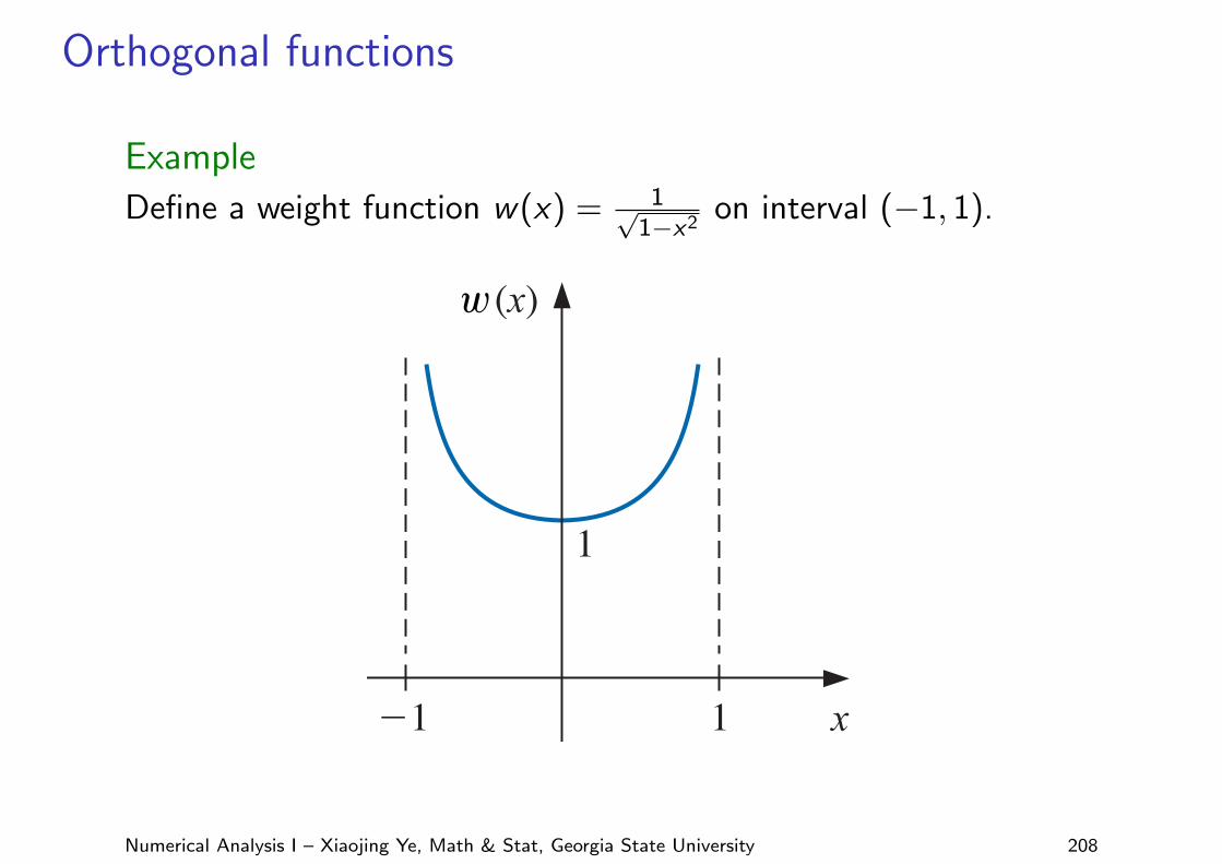
DefinitionAn integrable function w is called a weight function on theinterval I if w(x) ≥ 0, for all x ∈ I , but w(x) 6≡ 0 on anysubinterval of I .
Numerical Analysis I – Xiaojing Ye, Math & Stat, Georgia State University 207
Orthogonal functions
Example
Define a weight function w(x) = 1√1−x2
on interval (−1, 1).
514 C H A P T E R 8 Approximation Theory
Orthogonal Functions
To discuss general function approximation requires the introduction of the notions of weightfunctions and orthogonality.
Definition 8.4 An integrable function w is called a weight function on the interval I if w(x) ≥ 0, for allx in I , but w(x) ̸≡ 0 on any subinterval of I .
The purpose of a weight function is to assign varying degrees of importance to approx-imations on certain portions of the interval. For example, the weight function
w(x) = 1√1− x2
places less emphasis near the center of the interval (−1, 1) and more emphasis when |x| isnear 1 (see Figure 8.8). This weight function is used in the next section.
Suppose {φ0,φ1, . . . ,φn} is a set of linearly independent functions on [a, b] and w is aweight function for [a, b]. Given f ∈ C[a, b], we seek a linear combination
P(x) =n∑
k=0
akφk(x)
to minimize the error
E = E(a0, . . . , an) =∫ b
aw(x)
[f (x)−
n∑
k=0
akφk(x)]2
dx.
This problem reduces to the situation considered at the beginning of this section in the
Figure 8.8(x)
1!1
1
x
special case when w(x) ≡ 1 and φk(x) = xk , for each k = 0, 1, . . . , n.The normal equations associated with this problem are derived from the fact that for
each j = 0, 1, . . . , n,
0 = ∂E∂aj
= 2∫ b
aw(x)
[f (x)−
n∑
k=0
akφk(x)]φj(x) dx.
The system of normal equations can be written∫ b
aw(x)f (x)φj(x) dx =
n∑
k=0
ak
∫ b
aw(x)φk(x)φj(x) dx, for j = 0, 1, . . . , n.
If the functions φ0,φ1, . . . ,φn can be chosen so that∫ b
aw(x)φk(x)φj(x) dx =
{0, when j ̸= k,αj > 0, when j = k,
(8.7)
then the normal equations will reduce to∫ b
aw(x)f (x)φj(x) dx = aj
∫ b
aw(x)[φj(x)]2 dx = ajαj,
for each j = 0, 1, . . . , n. These are easily solved to give
aj = 1αj
∫ b
aw(x)f (x)φj(x) dx.
Hence the least squares approximation problem is greatly simplified when the functionsφ0,φ1, . . . ,φn are chosen to satisfy the orthogonality condition in Eq. (8.7). The remainderof this section is devoted to studying collections of this type.
The word orthogonal meansright-angled. So in a sense,orthogonal functions areperpendicular to one another.
Copyright 2010 Cengage Learning. All Rights Reserved. May not be copied, scanned, or duplicated, in whole or in part. Due to electronic rights, some third party content may be suppressed from the eBook and/or eChapter(s).Editorial review has deemed that any suppressed content does not materially affect the overall learning experience. Cengage Learning reserves the right to remove additional content at any time if subsequent rights restrictions require it.
Numerical Analysis I – Xiaojing Ye, Math & Stat, Georgia State University 208
Orthogonal functions
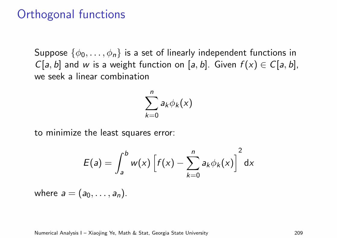
Suppose {φ0, . . . , φn} is a set of linearly independent functions inC [a, b] and w is a weight function on [a, b]. Given f (x) ∈ C [a, b],we seek a linear combination
n∑
k=0
akφk(x)
to minimize the least squares error:
E (a) =
∫ b
aw(x)
[f (x)−
n∑
k=0
akφk(x)]2
dx
where a = (a0, . . . , an).
Numerical Analysis I – Xiaojing Ye, Math & Stat, Georgia State University 209
Orthogonal functions
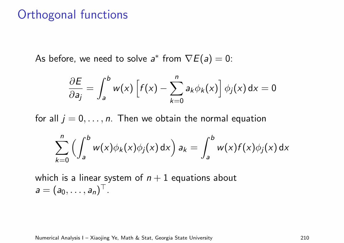
As before, we need to solve a∗ from ∇E (a) = 0:
∂E
∂aj=
∫ b
aw(x)
[f (x)−
n∑
k=0
akφk(x)]φj(x) dx = 0
for all j = 0, . . . , n. Then we obtain the normal equation
n∑
k=0
(∫ b
aw(x)φk(x)φj(x) dx
)ak =
∫ b
aw(x)f (x)φj(x) dx
which is a linear system of n + 1 equations abouta = (a0, . . . , an)>.
Numerical Analysis I – Xiaojing Ye, Math & Stat, Georgia State University 210
Orthogonal functions
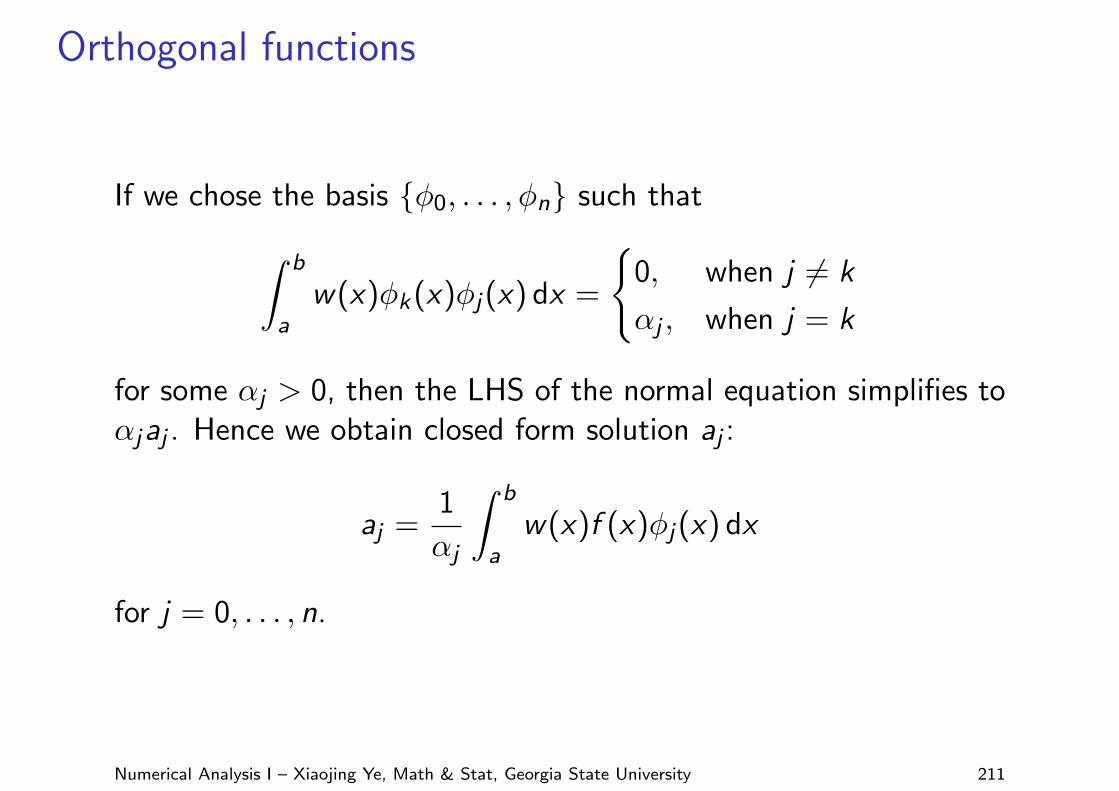
If we chose the basis {φ0, . . . , φn} such that
∫ b
aw(x)φk(x)φj(x) dx =
{0, when j 6= k
αj , when j = k
for some αj > 0, then the LHS of the normal equation simplifies toαjaj . Hence we obtain closed form solution aj :
aj =1
αj
∫ b
aw(x)f (x)φj(x) dx
for j = 0, . . . , n.
Numerical Analysis I – Xiaojing Ye, Math & Stat, Georgia State University 211
Orthogonal functions
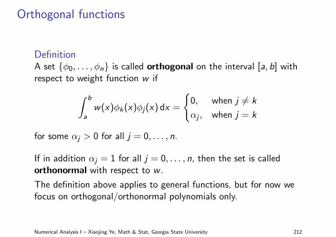
DefinitionA set {φ0, . . . , φn} is called orthogonal on the interval [a, b] withrespect to weight function w if
∫ b
aw(x)φk(x)φj(x) dx =
{0, when j 6= k
αj , when j = k
for some αj > 0 for all j = 0, . . . , n.
If in addition αj = 1 for all j = 0, . . . , n, then the set is calledorthonormal with respect to w .
The definition above applies to general functions, but for now wefocus on orthogonal/orthonormal polynomials only.
Numerical Analysis I – Xiaojing Ye, Math & Stat, Georgia State University 212
Gram-Schmidt process
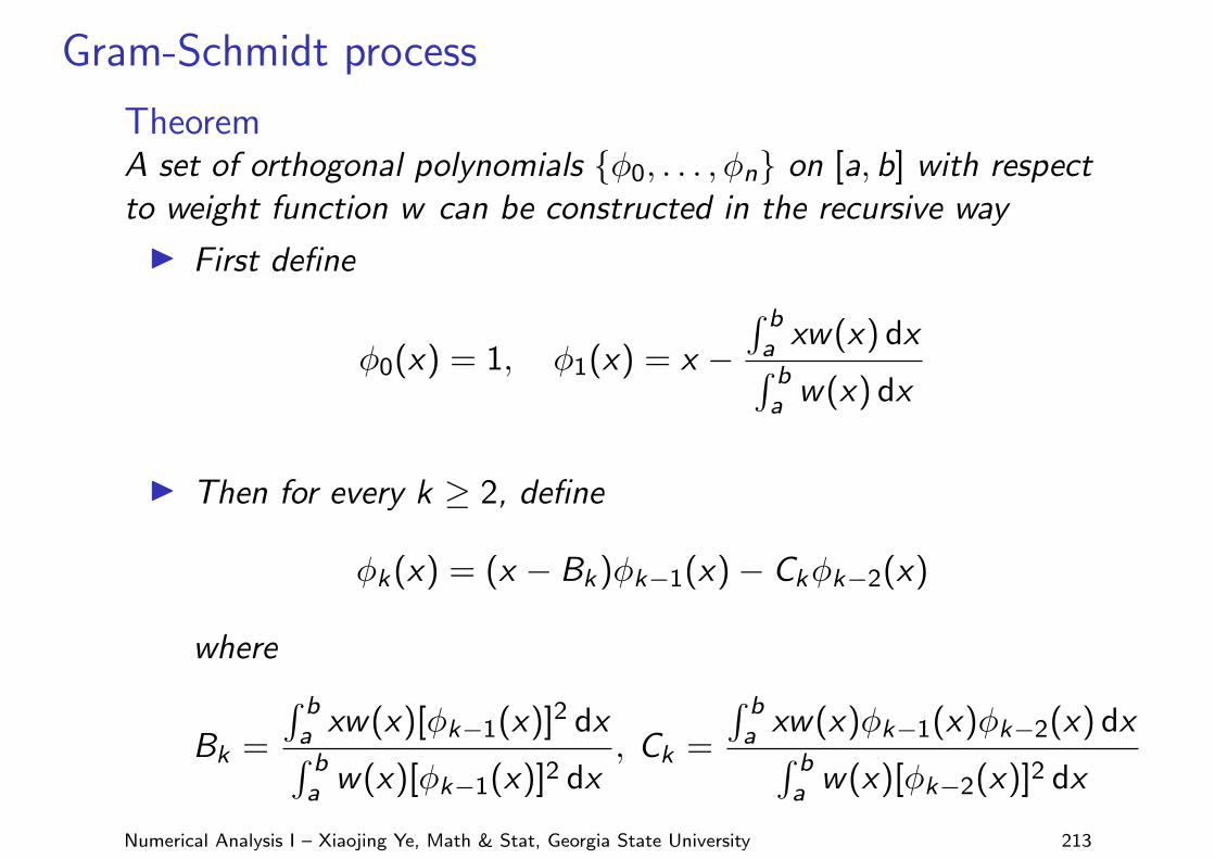
TheoremA set of orthogonal polynomials {φ0, . . . , φn} on [a, b] with respectto weight function w can be constructed in the recursive way
I First define
φ0(x) = 1, φ1(x) = x −∫ ba xw(x) dx∫ ba w(x) dx
I Then for every k ≥ 2, define
φk(x) = (x − Bk)φk−1(x)− Ckφk−2(x)
where
Bk =
∫ ba xw(x)[φk−1(x)]2 dx∫ ba w(x)[φk−1(x)]2 dx
, Ck =
∫ ba xw(x)φk−1(x)φk−2(x) dx∫ ba w(x)[φk−2(x)]2 dx
Numerical Analysis I – Xiaojing Ye, Math & Stat, Georgia State University 213
Orthogonal polynomials
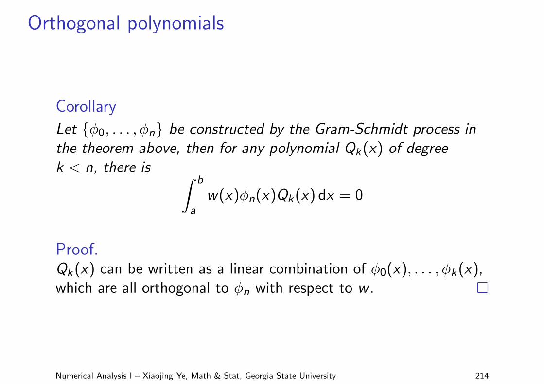
Corollary
Let {φ0, . . . , φn} be constructed by the Gram-Schmidt process inthe theorem above, then for any polynomial Qk(x) of degreek < n, there is ∫ b
aw(x)φn(x)Qk(x) dx = 0
Proof.Qk(x) can be written as a linear combination of φ0(x), . . . , φk(x),which are all orthogonal to φn with respect to w .
Numerical Analysis I – Xiaojing Ye, Math & Stat, Georgia State University 214
Legendre polynomials
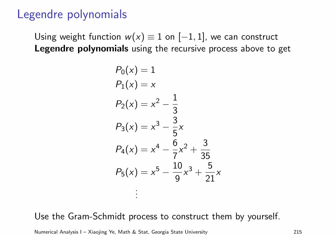
Using weight function w(x) ≡ 1 on [−1, 1], we can constructLegendre polynomials using the recursive process above to get
P0(x) = 1
P1(x) = x
P2(x) = x2 − 1
3
P3(x) = x3 − 3
5x
P4(x) = x4 − 6
7x2 +
3
35
P5(x) = x5 − 10
9x3 +
5
21x
...
Use the Gram-Schmidt process to construct them by yourself.
Numerical Analysis I – Xiaojing Ye, Math & Stat, Georgia State University 215
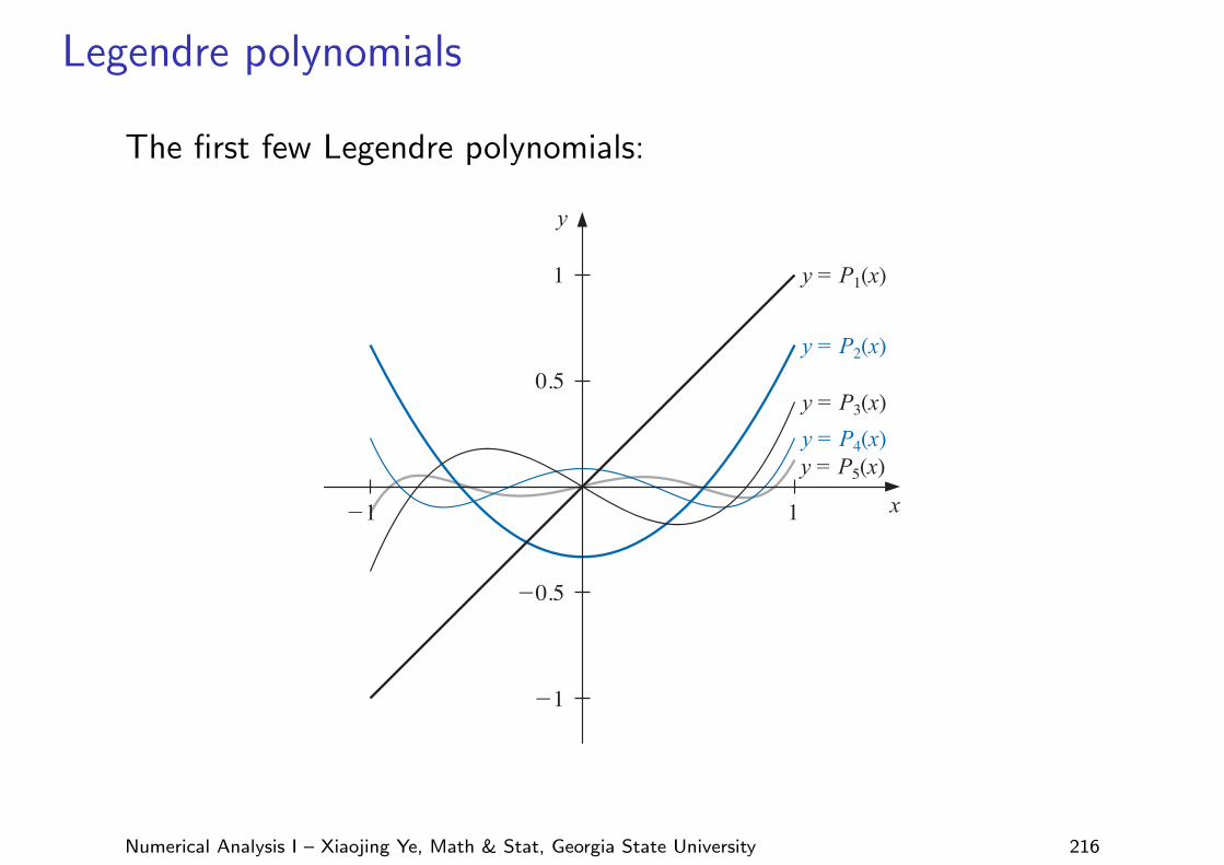
Legendre polynomials
The first few Legendre polynomials:8.2 Orthogonal Polynomials and Least Squares Approximation 517
Figure 8.9y
x
y = P1(x)
y = P2(x)
y = P3(x)y = P4(x)y = P5(x)
1
!1
!1
!0.5
0.5
1
For example, the Maple command int is used to compute the integrals B3 and C3:
B3 :=int(
x(x2 − 1
3
)2, x = −1..1
)
int((
x2 − 13
)2, x = −1..1
) ; C3 := int(x(x2 − 1
3
), x = −1..1
)
int(x2, x = −1..1)
0
415
Thus
P3(x) = xP2(x)−415
P1(x) = x3 − 13
x − 415
x = x3 − 35
x.
The next two Legendre polynomials are
P4(x) = x4 − 67
x2 + 335
and P5(x) = x5 − 109
x3 + 521
x. !
The Legendre polynomials were introduced in Section 4.7, where their roots, given onpage 232, were used as the nodes in Gaussian quadrature.
Copyright 2010 Cengage Learning. All Rights Reserved. May not be copied, scanned, or duplicated, in whole or in part. Due to electronic rights, some third party content may be suppressed from the eBook and/or eChapter(s).Editorial review has deemed that any suppressed content does not materially affect the overall learning experience. Cengage Learning reserves the right to remove additional content at any time if subsequent rights restrictions require it.
Numerical Analysis I – Xiaojing Ye, Math & Stat, Georgia State University 216
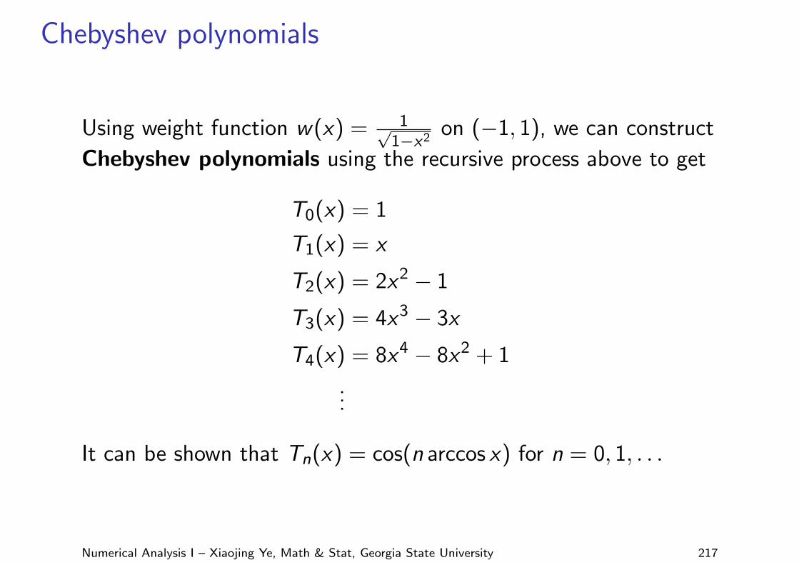
Chebyshev polynomials
Using weight function w(x) = 1√1−x2
on (−1, 1), we can construct
Chebyshev polynomials using the recursive process above to get
T0(x) = 1
T1(x) = x
T2(x) = 2x2 − 1
T3(x) = 4x3 − 3x
T4(x) = 8x4 − 8x2 + 1
...
It can be shown that Tn(x) = cos(n arccos x) for n = 0, 1, . . .
Numerical Analysis I – Xiaojing Ye, Math & Stat, Georgia State University 217
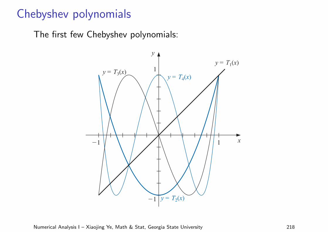
Chebyshev polynomials
The first few Chebyshev polynomials:
520 C H A P T E R 8 Approximation Theory
Figure 8.10
x
y = T1(x)
y = T2(x)
y = T3(x) y = T4(x)1
1
!1
!1
y
To show the orthogonality of the Chebyshev polynomials with respect to the weightfunction w(x) = (1− x2)−1/2, consider
∫ 1
−1
Tn(x)Tm(x)√1− x2
dx =∫ 1
−1
cos(n arccos x) cos(m arccos x)√1− x2
dx.
Reintroducing the substitution θ = arccos x gives
dθ = − 1√1− x2
dx
and∫ 1
−1
Tn(x)Tm(x)√1− x2
dx = −∫ 0
π
cos(nθ) cos(mθ) dθ =∫ π
0cos(nθ) cos(mθ) dθ .
Suppose n ̸= m. Since
cos(nθ) cos(mθ) = 12[cos(n + m)θ + cos(n− m)θ ],
we have∫ 1
−1
Tn(x)Tm(x)√1− x2
dx = 12
∫ π
0cos((n + m)θ) dθ + 1
2
∫ π
0cos((n− m)θ) dθ
=[
12(n + m)
sin((n + m)θ) + 12(n− m)
sin((n− m)θ)
]π
0= 0.
By a similar technique (see Exercise 9), we also have∫ 1
−1
[Tn(x)]2
√1− x2
dx = π
2, for each n ≥ 1. (8.10)
The Chebyshev polynomials are used to minimize approximation error. We will seehow they are used to solve two problems of this type:
Copyright 2010 Cengage Learning. All Rights Reserved. May not be copied, scanned, or duplicated, in whole or in part. Due to electronic rights, some third party content may be suppressed from the eBook and/or eChapter(s).Editorial review has deemed that any suppressed content does not materially affect the overall learning experience. Cengage Learning reserves the right to remove additional content at any time if subsequent rights restrictions require it.
Numerical Analysis I – Xiaojing Ye, Math & Stat, Georgia State University 218
Chebyshev polynomials
The Chebyshev polynomials Tn(x) of degree n ≥ 1 has n simplezeros in [−1, 1] (from right to left) at
x̄k = cos(2k − 1
2nπ), for each k = 1, 2, . . . , n
Moreover, Tn has maximum/minimum (from right to left) at
x̄ ′k = cos(kπ
n
)where Tn(x̄ ′k) = (−1)k for each k = 0, 1, 2, . . . , n
Therefore Tn(x) has n distinct roots and n + 1 extreme points on[−1, 1]. These 2n + 1 points, from right to left, are max, zero,min, zero, max ...
Numerical Analysis I – Xiaojing Ye, Math & Stat, Georgia State University 219
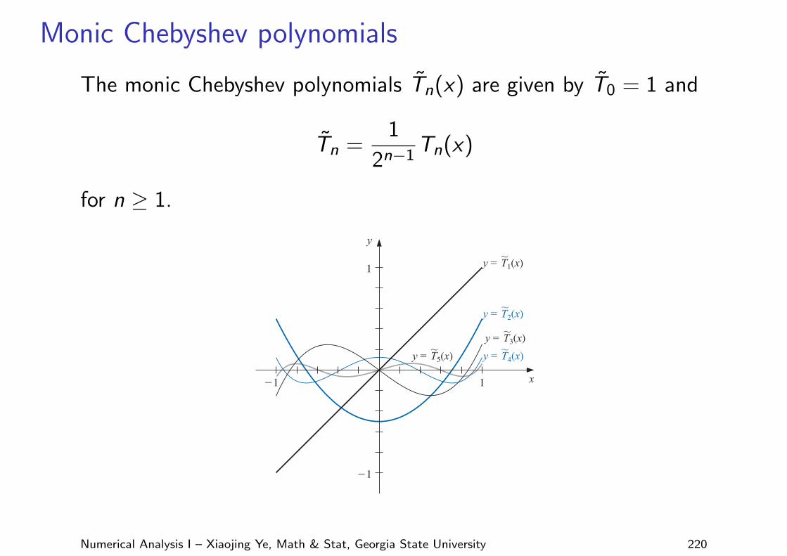
Monic Chebyshev polynomials
The monic Chebyshev polynomials T̃n(x) are given by T̃0 = 1 and
T̃n =1
2n−1Tn(x)
for n ≥ 1.
522 C H A P T E R 8 Approximation Theory
The recurrence relationship satisfied by the Chebyshev polynomials implies that
T̃2(x) = xT̃1(x)−12
T̃0(x) and (8.12)
T̃n+1(x) = xT̃n(x)−14
T̃n−1(x), for each n ≥ 2.
The graphs of T̃1, T̃2, T̃3, T̃4, and T̃5 are shown in Figure 8.11.
Figure 8.11
x1
1
!1
!1
y
y = T2(x)!
y = T1(x)!
y = T3(x)!
y = T4(x)!y = T5(x)
!
Because T̃n(x) is just a multiple of Tn(x), Theorem 8.9 implies that the zeros of T̃n(x)also occur at
x̄k = cos(
2k − 12n
π
), for each k = 1, 2, . . . , n,
and the extreme values of T̃n(x), for n ≥ 1, occur at
x̄′k = cos(
kπn
), with T̃n(x̄′k) = (−1)k
2n−1, for each k = 0, 1, 2, . . . , n. (8.13)
Let∏̃
n denote the set of all monic polynomials of degree n. The relation expressedin Eq. (8.13) leads to an important minimization property that distinguishes T̃n(x) from theother members of
∏̃n.
Theorem 8.10 The polynomials of the form T̃n(x), when n ≥ 1, have the property that
12n−1
= maxx∈[−1,1]
|T̃n(x)| ≤ maxx∈[−1, 1]
|Pn(x)|, for all Pn(x) ∈∏̃
n.
Moreover, equality occurs only if Pn ≡ T̃n.
Copyright 2010 Cengage Learning. All Rights Reserved. May not be copied, scanned, or duplicated, in whole or in part. Due to electronic rights, some third party content may be suppressed from the eBook and/or eChapter(s).Editorial review has deemed that any suppressed content does not materially affect the overall learning experience. Cengage Learning reserves the right to remove additional content at any time if subsequent rights restrictions require it.
Numerical Analysis I – Xiaojing Ye, Math & Stat, Georgia State University 220
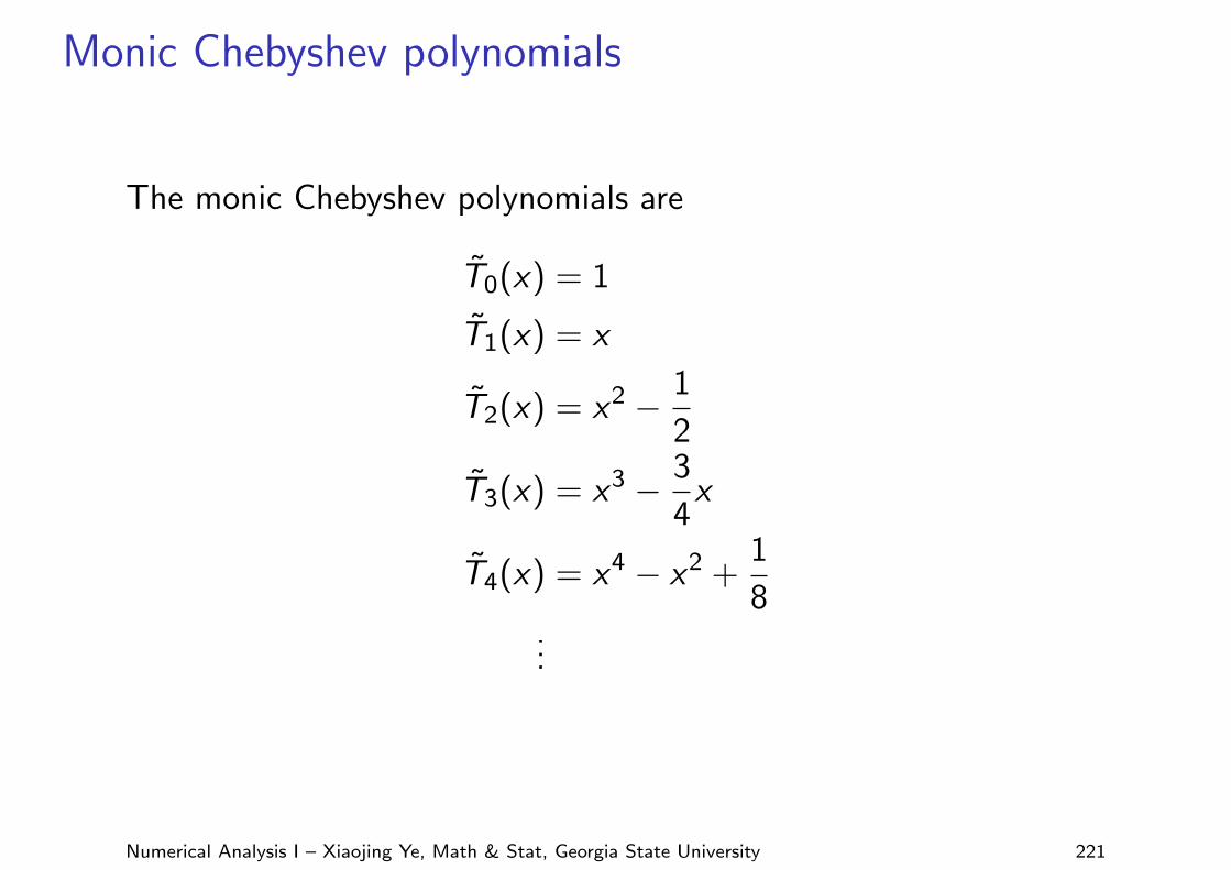
Monic Chebyshev polynomials
The monic Chebyshev polynomials are
T̃0(x) = 1
T̃1(x) = x
T̃2(x) = x2 − 1
2
T̃3(x) = x3 − 3
4x
T̃4(x) = x4 − x2 +1
8...
Numerical Analysis I – Xiaojing Ye, Math & Stat, Georgia State University 221
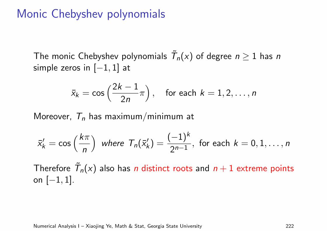
Monic Chebyshev polynomials
The monic Chebyshev polynomials T̃n(x) of degree n ≥ 1 has nsimple zeros in [−1, 1] at
x̄k = cos(2k − 1
2nπ), for each k = 1, 2, . . . , n
Moreover, Tn has maximum/minimum at
x̄ ′k = cos(kπ
n
)where Tn(x̄ ′k) =
(−1)k
2n−1, for each k = 0, 1, . . . , n
Therefore T̃n(x) also has n distinct roots and n + 1 extreme pointson [−1, 1].
Numerical Analysis I – Xiaojing Ye, Math & Stat, Georgia State University 222
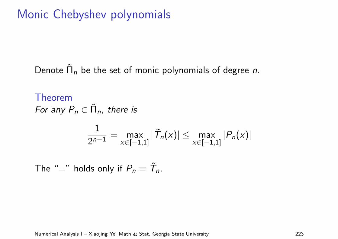
Monic Chebyshev polynomials
Denote Π̃n be the set of monic polynomials of degree n.
TheoremFor any Pn ∈ Π̃n, there is
1
2n−1= max
x∈[−1,1]|T̃n(x)| ≤ max
x∈[−1,1]|Pn(x)|
The “=” holds only if Pn ≡ T̃n.
Numerical Analysis I – Xiaojing Ye, Math & Stat, Georgia State University 223
Monic Chebyshev polynomials
Proof.Assume not, then ∃Pn(x) ∈ Π̃n, s.t. maxx∈[−1,1] |Pn(x)| < 1
2n−1 .
Let Q(x) := T̃n(x)− Pn(x). Since T̃n,Pn ∈ Π̃n, we know Q(x) isa ploynomial of degree at most n − 1. At the n + 1 extreme pointsx̄ ′k = cos
(kπn
)for k = 0, 1, . . . , n, there are
Q(x̄ ′k) = T̃n(x̄ ′k)− Pn(x̄ ′k) =(−1)k
2n−1− Pn(x̄ ′k)
Hence Q(x̄ ′k) > 0 when k is even and < 0 when k odd. Byintermediate value theorem, Q has at least n distinct roots,contradiction to deg(Q) ≤ n − 1.
Numerical Analysis I – Xiaojing Ye, Math & Stat, Georgia State University 224
Minimizing Lagrange interpolation error
Let x0, . . . , xn be n + 1 distinct points on [−1, 1] andf (x) ∈ Cn+1[−1, 1], recall that the Lagrange interpolatingpolynomial P(x) =
∑ni=0 f (xi )Li (x) satisfies
f (x)− P(x) =f (n+1)(ξ(x))
(n + 1)!(x − x0)(x − x1) · · · (x − xn)
for some ξ(x) ∈ (−1, 1) at every x ∈ [−1, 1].
We can control the size of (x − x0)(x − x1) · · · (x − xn) since itbelongs to Π̃n+1: set (x − x0)(x − x1) · · · (x − xn) = T̃n+1(x).
That is, set xk = cos(
2k−12n π
), the kth root of T̃n+1(x) for
k = 1, . . . , n + 1. This results in the minimalmaxx∈[−1,1] |(x − x0)(x − x1) · · · (x − xn)| = 1
2n .
Numerical Analysis I – Xiaojing Ye, Math & Stat, Georgia State University 225
Minimizing Lagrange interpolation error
Corollary
Let P(x) be the Lagrange interpolating polynomial with n + 1points chosen as the roots of T̃n+1(x), there is
maxx∈[−1,1]
|f (x)− P(x)| ≤ 1
2n(n + 1)!max
x∈[−1,1]|f (n+1)(x)|
Numerical Analysis I – Xiaojing Ye, Math & Stat, Georgia State University 226
Minimizing Lagrange interpolation error
If the interval of apporximation is on [a, b] instead of [−1, 1], wecan apply change of variable
x̃ =1
2[(b − a)x + (a + b)]
Hence, we can convert the roots x̄k on [−1, 1] to x̃k on [a, b],
Numerical Analysis I – Xiaojing Ye, Math & Stat, Georgia State University 227
Minimizing Lagrange interpolation error
Example
Let f (x) = xex on [0, 1.5]. Find the Lagrange interpolatingpolynomial using
1. the 4 equally spaced points 0, 0.5, 1, 1.5.
2. the 4 points transformed from roots of T̃4.
Numerical Analysis I – Xiaojing Ye, Math & Stat, Georgia State University 228

Minimizing Lagrange interpolation error
Solution. For each of the four points
x0 = 0, x1 = 0.5, x2 = 1, x3 = 1.5, we obtain Li (x) =∏
j 6=i (x−xj )∏j 6=i (xi−xj )
for
i = 0, 1, 2, 3:
L0(x) = −1.3333x3 + 4.0000x2 − 3.6667x + 1,
L1(x) = 4.0000x3 − 10.000x2 + 6.0000x ,
L2(x) = −4.0000x3 + 8.0000x2 − 3.0000x ,
L3(x) = 1.3333x3 − 2.000x2 + 0.66667x
so the Lagrange interpolating polynomial is
P3(x) =3∑
i=0
f (xi )Li (x) = 1.3875x3 + 0.057570x2 + 1.2730x .
Numerical Analysis I – Xiaojing Ye, Math & Stat, Georgia State University 229
Minimizing Lagrange interpolation error
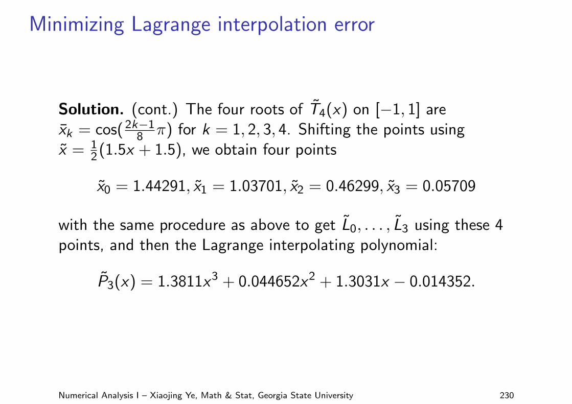
Solution. (cont.) The four roots of T̃4(x) on [−1, 1] arex̄k = cos( 2k−1
8 π) for k = 1, 2, 3, 4. Shifting the points usingx̃ = 1
2 (1.5x + 1.5), we obtain four points
x̃0 = 1.44291, x̃1 = 1.03701, x̃2 = 0.46299, x̃3 = 0.05709
with the same procedure as above to get L̃0, . . . , L̃3 using these 4points, and then the Lagrange interpolating polynomial:
P̃3(x) = 1.3811x3 + 0.044652x2 + 1.3031x − 0.014352.
Numerical Analysis I – Xiaojing Ye, Math & Stat, Georgia State University 230
Minimizing Lagrange interpolation error
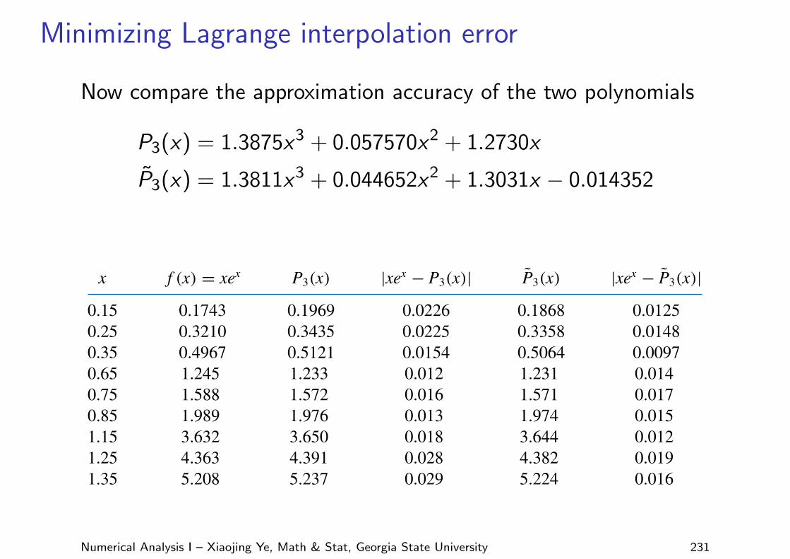
Now compare the approximation accuracy of the two polynomials
P3(x) = 1.3875x3 + 0.057570x2 + 1.2730x
P̃3(x) = 1.3811x3 + 0.044652x2 + 1.3031x − 0.014352
8.3 Chebyshev Polynomials and Economization of Power Series 525
The functional values required for these polynomials are given in the last two columnsof Table 8.7. The interpolation polynomial of degree at most 3 is
P̃3(x) = 1.3811x3 + 0.044652x2 + 1.3031x−0.014352.
Table 8.7 x f (x) = xex x̃ f (x̃) = xex
x0 = 0.0 0.00000 x̃0 = 1.44291 6.10783x1 = 0.5 0.824361 x̃1 = 1.03701 2.92517x2 = 1.0 2.71828 x̃2 = 0.46299 0.73560x3 = 1.5 6.72253 x̃3 = 0.05709 0.060444
For comparison, Table 8.8 lists various values of x, together with the values off (x), P3(x), and P̃3(x). It can be seen from this table that, although the error using P3(x) isless than using P̃3(x) near the middle of the table, the maximum error involved with usingP̃3(x), 0.0180, is considerably less than when using P3(x), which gives the error 0.0290.(See Figure 8.12.)
Table 8.8 x f (x) = xex P3(x) |xex−P3(x)| P̃3(x) |xex−P̃3(x)|0.15 0.1743 0.1969 0.0226 0.1868 0.01250.25 0.3210 0.3435 0.0225 0.3358 0.01480.35 0.4967 0.5121 0.0154 0.5064 0.00970.65 1.245 1.233 0.012 1.231 0.0140.75 1.588 1.572 0.016 1.571 0.0170.85 1.989 1.976 0.013 1.974 0.0151.15 3.632 3.650 0.018 3.644 0.0121.25 4.363 4.391 0.028 4.382 0.0191.35 5.208 5.237 0.029 5.224 0.016
Figure 8.12
y = P3(x)!
y ! xex
0.5 1.0 1.5
6
5
4
3
2
1
y
x
Copyright 2010 Cengage Learning. All Rights Reserved. May not be copied, scanned, or duplicated, in whole or in part. Due to electronic rights, some third party content may be suppressed from the eBook and/or eChapter(s).Editorial review has deemed that any suppressed content does not materially affect the overall learning experience. Cengage Learning reserves the right to remove additional content at any time if subsequent rights restrictions require it.
Numerical Analysis I – Xiaojing Ye, Math & Stat, Georgia State University 231
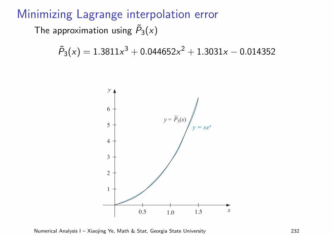
Minimizing Lagrange interpolation errorThe approximation using P̃3(x)
P̃3(x) = 1.3811x3 + 0.044652x2 + 1.3031x − 0.014352
8.3 Chebyshev Polynomials and Economization of Power Series 525
The functional values required for these polynomials are given in the last two columnsof Table 8.7. The interpolation polynomial of degree at most 3 is
P̃3(x) = 1.3811x3 + 0.044652x2 + 1.3031x − 0.014352.
Table 8.7 x f (x) = xex x̃ f (x̃) = xex
x0 = 0.0 0.00000 x̃0 = 1.44291 6.10783x1 = 0.5 0.824361 x̃1 = 1.03701 2.92517x2 = 1.0 2.71828 x̃2 = 0.46299 0.73560x3 = 1.5 6.72253 x̃3 = 0.05709 0.060444
For comparison, Table 8.8 lists various values of x, together with the values off (x), P3(x), and P̃3(x). It can be seen from this table that, although the error using P3(x) isless than using P̃3(x) near the middle of the table, the maximum error involved with usingP̃3(x), 0.0180, is considerably less than when using P3(x), which gives the error 0.0290.(See Figure 8.12.)
Table 8.8 x f (x) = xex P3(x) |xex − P3(x)| P̃3(x) |xex − P̃3(x)|0.15 0.1743 0.1969 0.0226 0.1868 0.01250.25 0.3210 0.3435 0.0225 0.3358 0.01480.35 0.4967 0.5121 0.0154 0.5064 0.00970.65 1.245 1.233 0.012 1.231 0.0140.75 1.588 1.572 0.016 1.571 0.0170.85 1.989 1.976 0.013 1.974 0.0151.15 3.632 3.650 0.018 3.644 0.0121.25 4.363 4.391 0.028 4.382 0.0191.35 5.208 5.237 0.029 5.224 0.016
Figure 8.12
y = P3(x)!
y ! xex
0.5 1.0 1.5
6
5
4
3
2
1
y
x
Copyright 2010 Cengage Learning. All Rights Reserved. May not be copied, scanned, or duplicated, in whole or in part. Due to electronic rights, some third party content may be suppressed from the eBook and/or eChapter(s).Editorial review has deemed that any suppressed content does not materially affect the overall learning experience. Cengage Learning reserves the right to remove additional content at any time if subsequent rights restrictions require it.
Numerical Analysis I – Xiaojing Ye, Math & Stat, Georgia State University 232
Reducing the degree of approximating polynomials
As Chebyshev polynomials are efficient in approximating functions,we may use approximating polynomials of smaller degree for agiven error tolerance.
For example, let Qn(x) = a0 + · · ·+ anxn be a polynomial ofdegree n on [−1, 1]. Can we find a polynomial of degree n − 1 toapproximate Qn?
Numerical Analysis I – Xiaojing Ye, Math & Stat, Georgia State University 233
Reducing the degree of approximating polynomials
So our goal is to find Pn−1(x) ∈ Πn−1 such that
maxx∈[−1,1]
|Qn(x)− Pn−1(x)|
is minimized. Note that 1an
(Qn(x)− Pn−1(x)) ∈ Π̃n, we know the
best choice is 1an
(Qn(x)− Pn−1(x)) = T̃n(x), i.e.,
Pn−1 = Qn − anT̃n. In this case, we have approximation error
maxx∈[−1,1]
|Qn(x)− Pn−1(x)| = maxx∈[−1,1]
|anT̃n| =|an|2n−1
Numerical Analysis I – Xiaojing Ye, Math & Stat, Georgia State University 234
Reducing the degree of approximating polynomials
Example
Recall that Q4(x) be the 4th Maclaurin polynomial of f (x) = ex
about 0 on [−1, 1]. That is
Q4(x) = 1 + x +x2
2+
x3
6+
x4
24
which has a4 = 124 and truncation error
|R4(x)| = | f(5)(ξ(x))x5
5!| = |e
ξ(x)x5
5!| ≤ e
5!≈ 0.023
for x ∈ (−1, 1). Given error tolerance 0.05, find the polynomial ofsmall degree to approximate f (x).
Numerical Analysis I – Xiaojing Ye, Math & Stat, Georgia State University 235
Reducing the degree of approximating polynomials
Solution. Let’s first try Π3. Note that T̃4(x) = x4 − x2 + 18 , so we
can set
P3(x) = Q4(x)− a4T̃4(x)
=(
1 + x +x2
2+
x3
6+
x4
24
)− 1
24
(x4 − x2 +
1
8
)
=191
192+ x +
13
24x2 +
1
6x3 ∈ Π3
Therefore, the approximating error is bounded by
|f (x)− P3(x)| ≤ |f (x)− Q4(x)|+ |Q4(x)− P3(x)|
≤ 0.023 +|a4|23
= 0.023 +1
192≤ 0.0283.
Numerical Analysis I – Xiaojing Ye, Math & Stat, Georgia State University 236
Reducing the degree of approximating polynomials
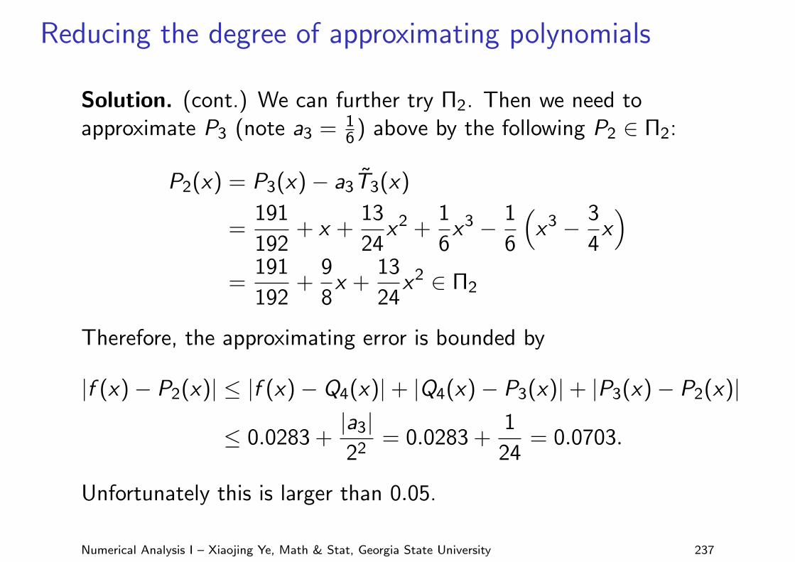
Solution. (cont.) We can further try Π2. Then we need toapproximate P3 (note a3 = 1
6 ) above by the following P2 ∈ Π2:
P2(x) = P3(x)− a3T̃3(x)
=191
192+ x +
13
24x2 +
1
6x3 − 1
6
(x3 − 3
4x)
=191
192+
9
8x +
13
24x2 ∈ Π2
Therefore, the approximating error is bounded by
|f (x)− P2(x)| ≤ |f (x)− Q4(x)|+ |Q4(x)− P3(x)|+ |P3(x)− P2(x)|
≤ 0.0283 +|a3|22
= 0.0283 +1
24= 0.0703.
Unfortunately this is larger than 0.05.
Numerical Analysis I – Xiaojing Ye, Math & Stat, Georgia State University 237
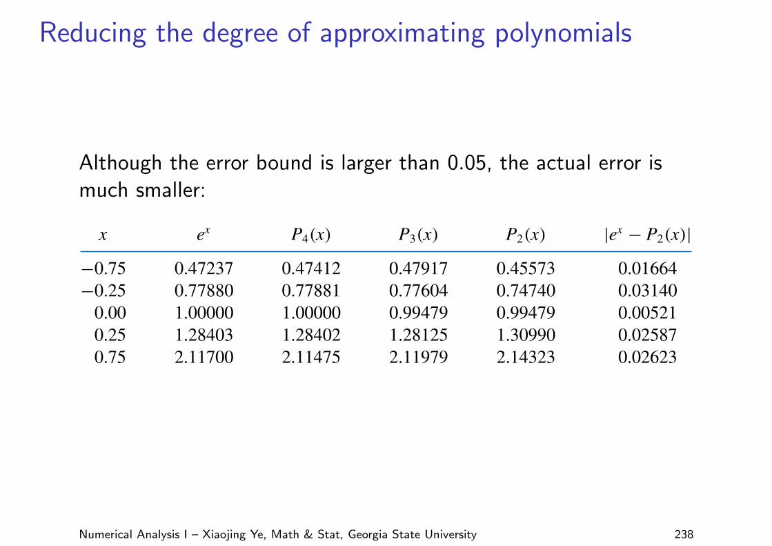
Reducing the degree of approximating polynomials
Although the error bound is larger than 0.05, the actual error ismuch smaller:
8.3 Chebyshev Polynomials and Economization of Power Series 527
With this choice, we have
|P4(x)− P3(x)| = |a4T̃4(x)| ≤1
24· 1
23= 1
192≤ 0.0053.
Adding this error bound to the bound for the Maclaurin truncation error gives
0.023 + 0.0053 = 0.0283,
which is within the permissible error of 0.05.
The polynomial of degree 2 or less that best uniformly approximates P3(x) on [−1, 1] is
P2(x) = P3(x)−16
T̃3(x)
= 191192
+ x + 1324
x2 + 16
x3 − 16(x3 − 3
4x) = 191
192+ 9
8x + 13
24x2.
However,
|P3(x)− P2(x)| =∣∣∣∣16
T̃3(x)∣∣∣∣ = 1
6
(12
)2
= 124≈ 0.042,
which—when added to the already accumulated error bound of 0.0283—exceeds the tol-erance of 0.05. Consequently, the polynomial of least degree that best approximates ex on[−1, 1] with an error bound of less than 0.05 is
P3(x) = 191192
+ x + 1324
x2 + 16
x3.
Table 8.9 lists the function and the approximating polynomials at various points in [−1, 1].Note that the tabulated entries for P2 are well within the tolerance of 0.05, even though theerror bound for P2(x) exceeded the tolerance. !
Table 8.9 x ex P4(x) P3(x) P2(x) |ex − P2(x)|−0.75 0.47237 0.47412 0.47917 0.45573 0.01664−0.25 0.77880 0.77881 0.77604 0.74740 0.03140
0.00 1.00000 1.00000 0.99479 0.99479 0.005210.25 1.28403 1.28402 1.28125 1.30990 0.025870.75 2.11700 2.11475 2.11979 2.14323 0.02623
E X E R C I S E S E T 8.3
1. Use the zeros of T̃3 to construct an interpolating polynomial of degree 2 for the following functionson the interval [−1, 1].a. f (x) = ex b. f (x) = sin x c. f (x) = ln(x + 2) d. f (x) = x4
2. Use the zeros of T̃4 to construct an interpolating polynomial of degree 3 for the functions in Exercise 1.3. Find a bound for the maximum error of the approximation in Exercise 1 on the interval [−1, 1].4. Repeat Exercise 3 for the approximations computed in Exercise 3.
Copyright 2010 Cengage Learning. All Rights Reserved. May not be copied, scanned, or duplicated, in whole or in part. Due to electronic rights, some third party content may be suppressed from the eBook and/or eChapter(s).Editorial review has deemed that any suppressed content does not materially affect the overall learning experience. Cengage Learning reserves the right to remove additional content at any time if subsequent rights restrictions require it.
Numerical Analysis I – Xiaojing Ye, Math & Stat, Georgia State University 238
Pros and cons of polynomial approxiamtion
Advantages:
I Polynomials can approximate continuous function to arbitraryaccuracy;
I Polynomials are easy to evaluate;
I Derivatives and integrals are easy to compute.
Disadvantages:
I Significant oscillations;
I Large max absolute error in approximating;
I Not accurate when approximating discontinuous functions.
Numerical Analysis I – Xiaojing Ye, Math & Stat, Georgia State University 239