Linear Regression with varying noise - Penn … › ~cis520 › lectures › more...Title...
16
Slide 33 Copyright © 2001, 2003, Andrew W. Moore Linear Regression with varying noise Heteroscedasticity...
Transcript of Linear Regression with varying noise - Penn … › ~cis520 › lectures › more...Title...
Slide 33 Copyright © 2001, 2003, Andrew W. Moore
Linear Regression with varying noise
Heteroscedasticity...
Slide 34 Copyright © 2001, 2003, Andrew W. Moore
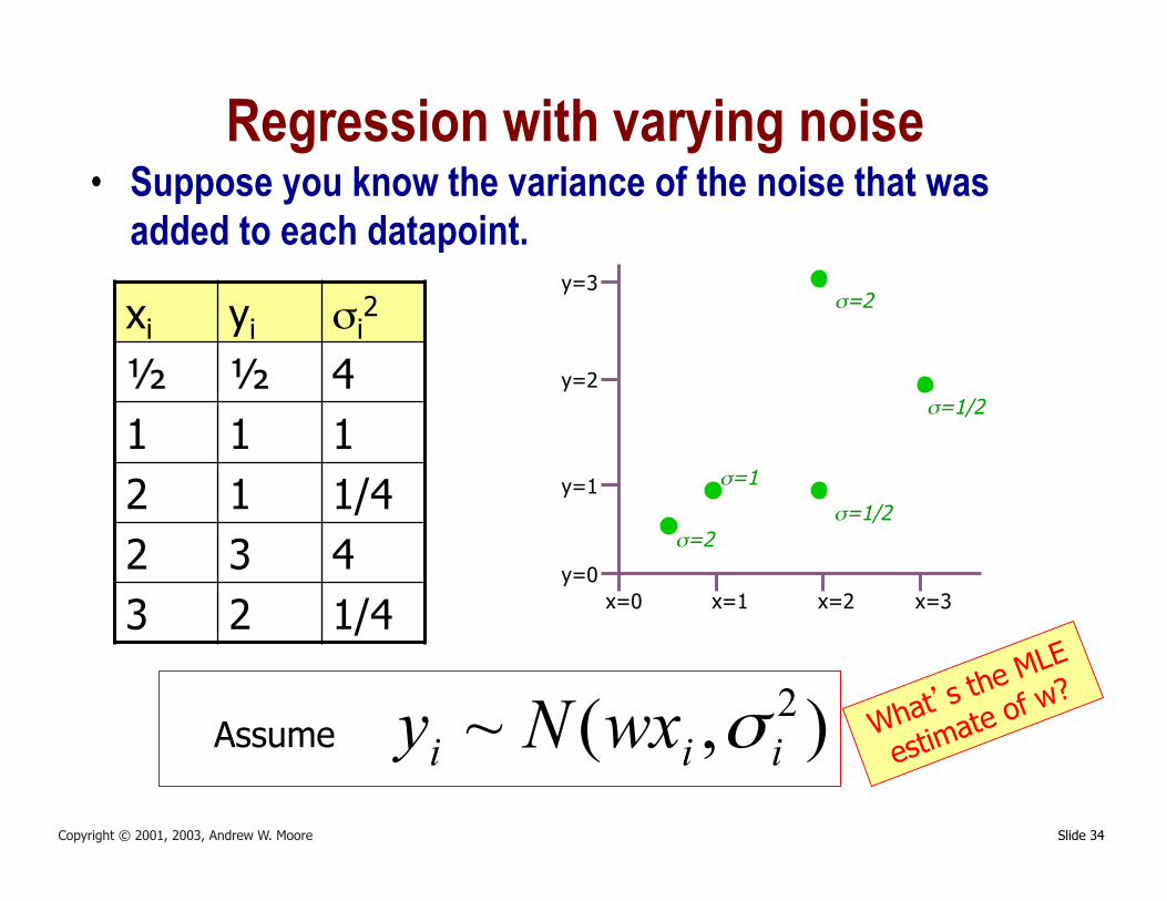
Regression with varying noise • Suppose you know the variance of the noise that was
added to each datapoint.
x=0 x=3 x=2 x=1 y=0
y=3
y=2
y=1
σ=1/2
σ=2
σ=1
σ=1/2
σ=2 xi yi σi2
½ ½ 4
1 1 1
2 1 1/4
2 3 4
3 2 1/4
),(~ 2iii wxNy σAssume
Slide 35 Copyright © 2001, 2003, Andrew W. Moore
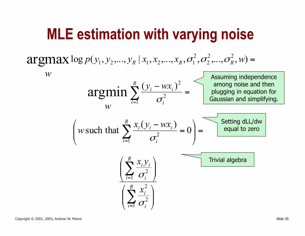
MLE estimation with varying noise =),,...,,,,...,,|,...,,(log 22
2212121argmax wxxxyyyp
wRRR σσσ
=−
∑=
R
i i
ii wxy
w 12
2)(argminσ
=⎟⎟⎠
⎞⎜⎜⎝
⎛=
−∑=
0)(such that 1
2
R
i i
iii wxyxwσ
⎟⎟⎠
⎞⎜⎜⎝
⎛
⎟⎟⎠
⎞⎜⎜⎝
⎛
∑
∑
=
=
R
i i
i
R
i i
ii
x
yx
12
21
2
σ
σ
Assuming independence among noise and then
plugging in equation for Gaussian and simplifying.
Setting dLL/dw equal to zero
Trivial algebra
Slide 36 Copyright © 2001, 2003, Andrew W. Moore
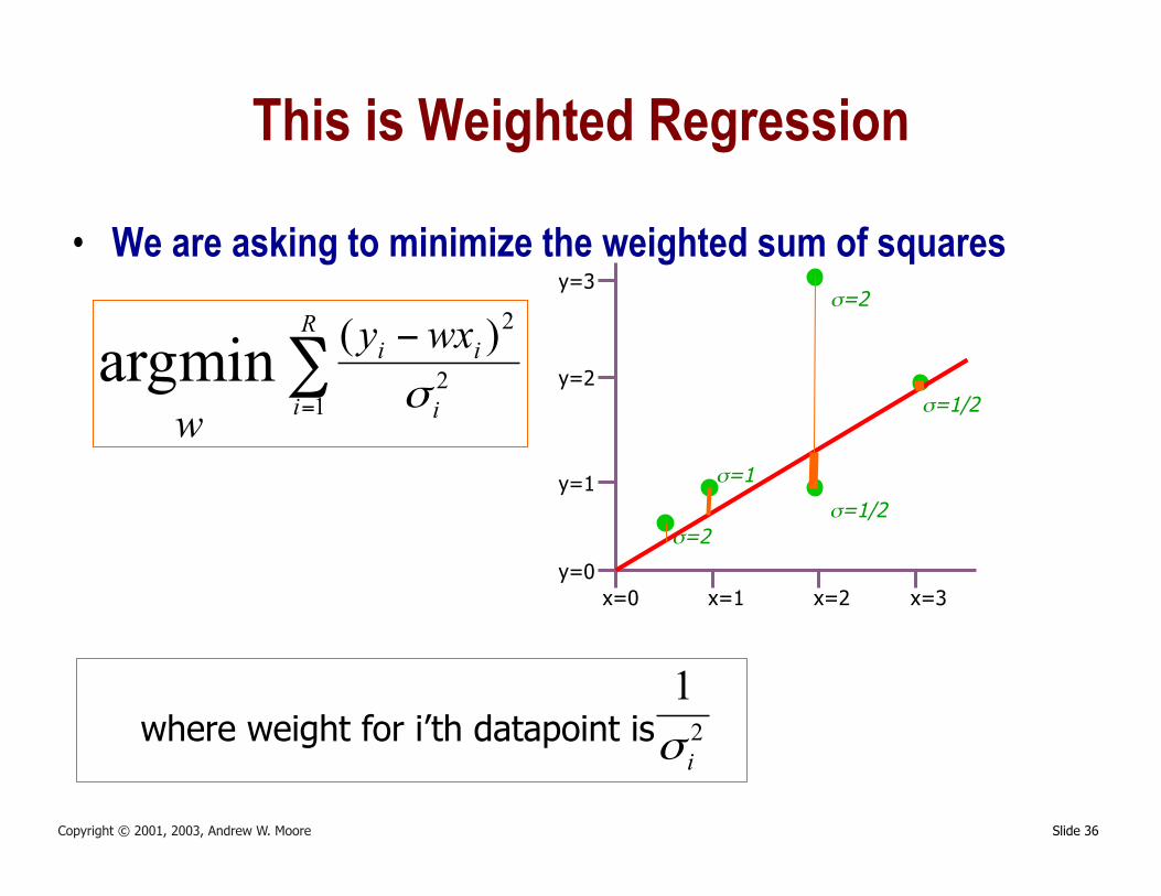
This is Weighted Regression
• We are asking to minimize the weighted sum of squares
x=0 x=3 x=2 x=1 y=0
y=3
y=2
y=1
σ=1/2
σ=2
σ=1
σ=1/2
σ=2
∑=
−R
i i
ii wxy
w 12
2)(argminσ
2
1
iσwhere weight for i’th datapoint is
Slide 37 Copyright © 2001, 2003, Andrew W. Moore
Non-linear Regression
Slide 38 Copyright © 2001, 2003, Andrew W. Moore
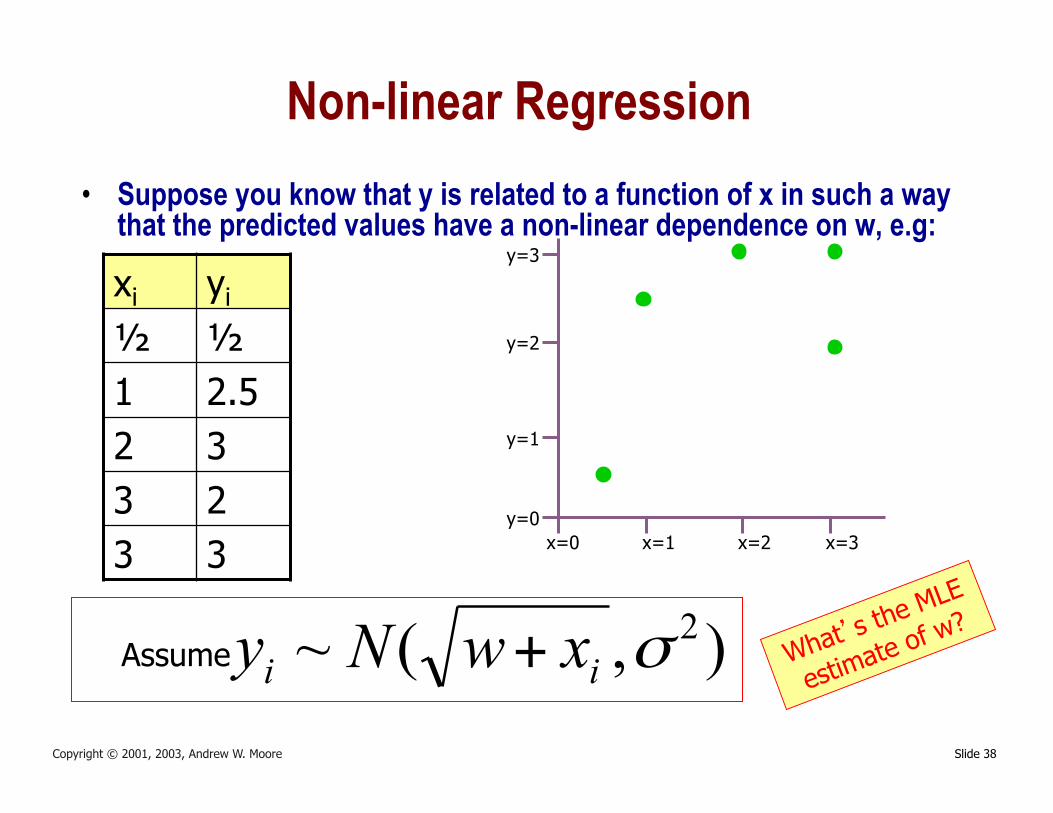
Non-linear Regression • Suppose you know that y is related to a function of x in such a way
that the predicted values have a non-linear dependence on w, e.g:
x=0 x=3 x=2 x=1 y=0
y=3
y=2
y=1
xi yi
½ ½ 1 2.5 2 3 3 2 3 3
),(~ 2σii xwNy +Assume
Slide 39 Copyright © 2001, 2003, Andrew W. Moore
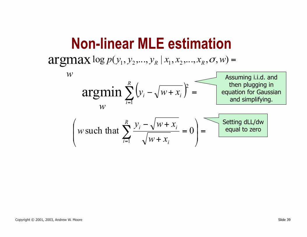
Non-linear MLE estimation =),,,...,,|,...,,(log 2121argmax wxxxyyyp
wRR σ
( ) =+−∑=
R
iii xwy
w 1
2argmin
=⎟⎟⎠
⎞⎜⎜⎝
⎛=
+
+−∑=
0such that 1
R
i i
ii
xwxwy
w
Assuming i.i.d. and then plugging in
equation for Gaussian and simplifying.
Setting dLL/dw equal to zero
Slide 40 Copyright © 2001, 2003, Andrew W. Moore
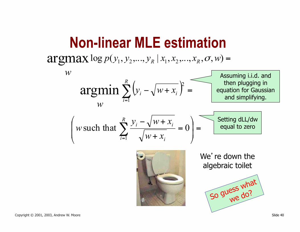
Non-linear MLE estimation =),,,...,,|,...,,(log 2121argmax wxxxyyyp
wRR σ
( ) =+−∑=
R
iii xwy
w 1
2argmin
=⎟⎟⎠
⎞⎜⎜⎝
⎛=
+
+−∑=
0such that 1
R
i i
ii
xwxwy
w
Assuming i.i.d. and then plugging in
equation for Gaussian and simplifying.
Setting dLL/dw equal to zero
We’re down the algebraic toilet
So guess what
we do?
Slide 41 Copyright © 2001, 2003, Andrew W. Moore
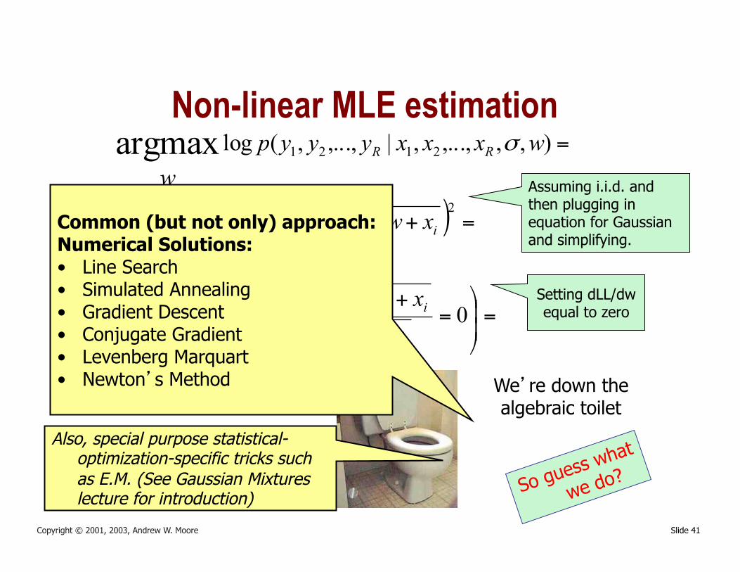
Non-linear MLE estimation =),,,...,,|,...,,(log 2121argmax wxxxyyyp
wRR σ
( ) =+−∑=
R
iii xwy
w 1
2argmin
=⎟⎟⎠
⎞⎜⎜⎝
⎛=
+
+−∑=
0such that 1
R
i i
ii
xwxwy
w
Assuming i.i.d. and then plugging in equation for Gaussian and simplifying.
Setting dLL/dw equal to zero
We’re down the algebraic toilet
So guess what
we do?
Common (but not only) approach: Numerical Solutions: • Line Search • Simulated Annealing • Gradient Descent • Conjugate Gradient • Levenberg Marquart • Newton’s Method
Also, special purpose statistical-optimization-specific tricks such as E.M. (See Gaussian Mixtures lecture for introduction)
Slide 42 Copyright © 2001, 2003, Andrew W. Moore
Polynomial Regression
Slide 43 Copyright © 2001, 2003, Andrew W. Moore
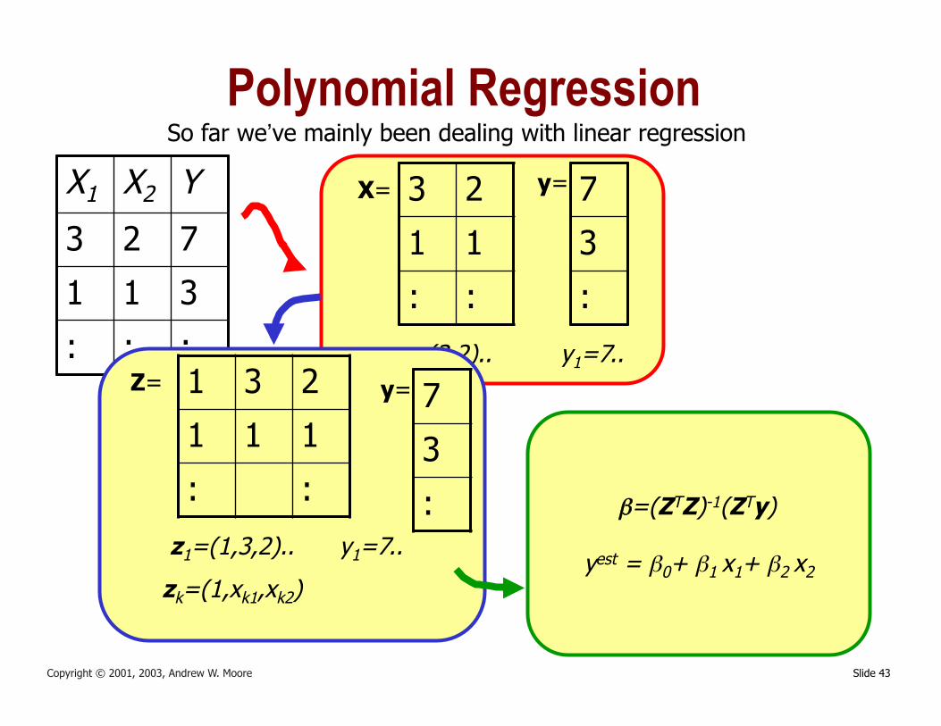
Polynomial Regression So far we’ve mainly been dealing with linear regression
X1 X2 Y
3 2 7
1 1 3
: : :
3 2
1 1
: :
7
3
:
X= y=
x1=(3,2).. y1=7.. 1 3 2
1 1 1
: :
7
3
:
Z= y=
z1=(1,3,2)..
zk=(1,xk1,xk2)
y1=7..
β=(ZTZ)-1(ZTy)
yest = β0+ β1 x1+ β2 x2
Slide 44 Copyright © 2001, 2003, Andrew W. Moore
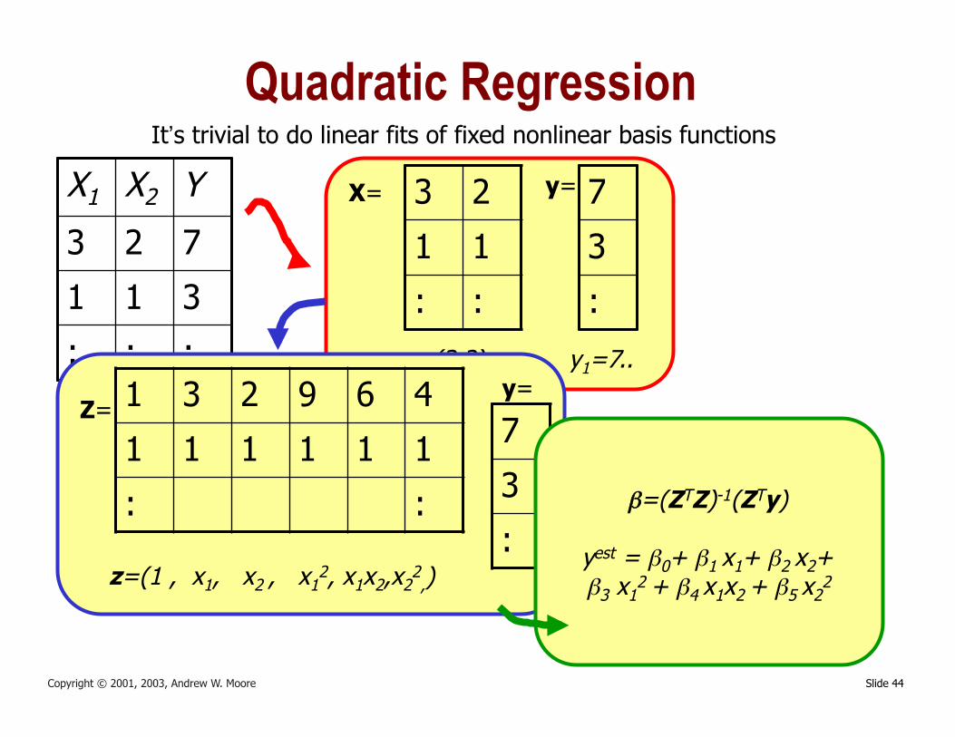
Quadratic Regression It’s trivial to do linear fits of fixed nonlinear basis functions
X1 X2 Y
3 2 7
1 1 3
: : :
3 2
1 1
: :
7
3
:
X= y=
x1=(3,2).. y1=7.. 1 3 2 9 6 4
1 1 1 1 1 1
: :
7
3
:
Z= y=
z=(1 , x1, x2 , x12, x1x2,x2
2,)
β=(ZTZ)-1(ZTy)
yest = β0+ β1 x1+ β2 x2+ β3 x1
2 + β4 x1x2 + β5 x22
Slide 45 Copyright © 2001, 2003, Andrew W. Moore
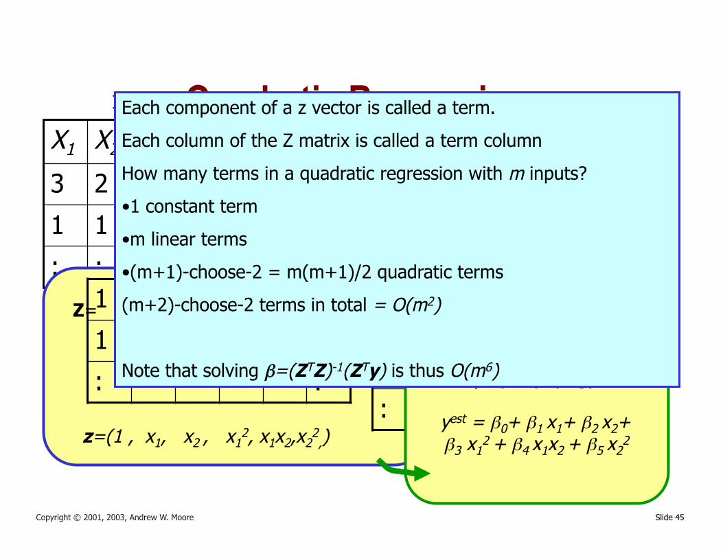
Quadratic Regression It’s trivial to do linear fits of fixed nonlinear basis functions
X1 X2 Y
3 2 7
1 1 3
: : :
3 2
1 1
: :
7
3
:
X= y=
x1=(3,2).. y1=7.. 1 3 2 9 6 4
1 1 1 1 1 1
: :
7
3
:
Z= y=
z=(1 , x1, x2 , x12, x1x2,x2
2,)
β=(ZTZ)-1(ZTy)
yest = β0+ β1 x1+ β2 x2+ β3 x1
2 + β4 x1x2 + β5 x22
Each component of a z vector is called a term.
Each column of the Z matrix is called a term column
How many terms in a quadratic regression with m inputs?
• 1 constant term
• m linear terms
• (m+1)-choose-2 = m(m+1)/2 quadratic terms
(m+2)-choose-2 terms in total = O(m2)
Note that solving β=(ZTZ)-1(ZTy) is thus O(m6)
Slide 46 Copyright © 2001, 2003, Andrew W. Moore
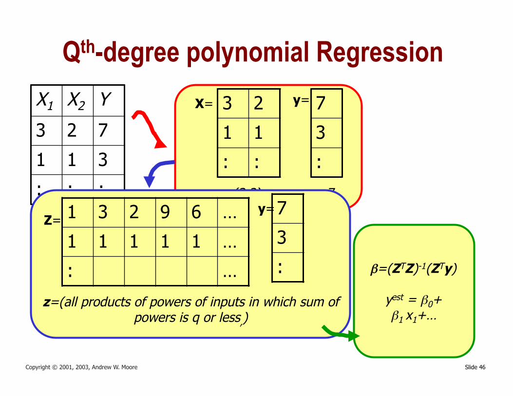
Qth-degree polynomial Regression X1 X2 Y
3 2 7
1 1 3
: : :
3 2
1 1
: :
7
3
:
X= y=
x1=(3,2).. y1=7.. 1 3 2 9 6 …
1 1 1 1 1 …
: …
7
3
:
Z= y=
z=(all products of powers of inputs in which sum of powers is q or less,)
β=(ZTZ)-1(ZTy)
yest = β0+ β1 x1+…
Slide 47 Copyright © 2001, 2003, Andrew W. Moore
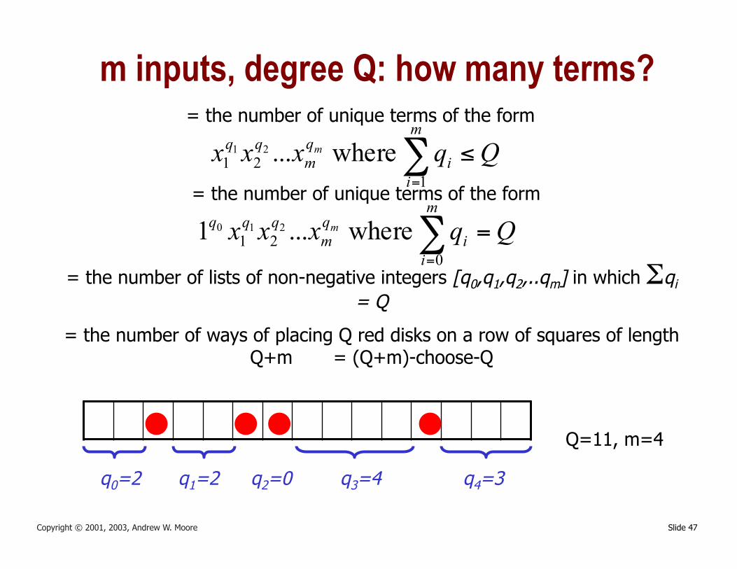
m inputs, degree Q: how many terms? = the number of unique terms of the form
Qqxxxm
ii
qm
qq m ≤∑=1
21 where...21
Qqxxxm
ii
qm
qqq m =∑=0
21 where...1 210
= the number of unique terms of the form
= the number of lists of non-negative integers [q0,q1,q2,..qm] in which Σqi = Q
= the number of ways of placing Q red disks on a row of squares of length Q+m = (Q+m)-choose-Q
Q=11, m=4
q0=2 q2=0 q1=2 q3=4 q4=3
Slide 48
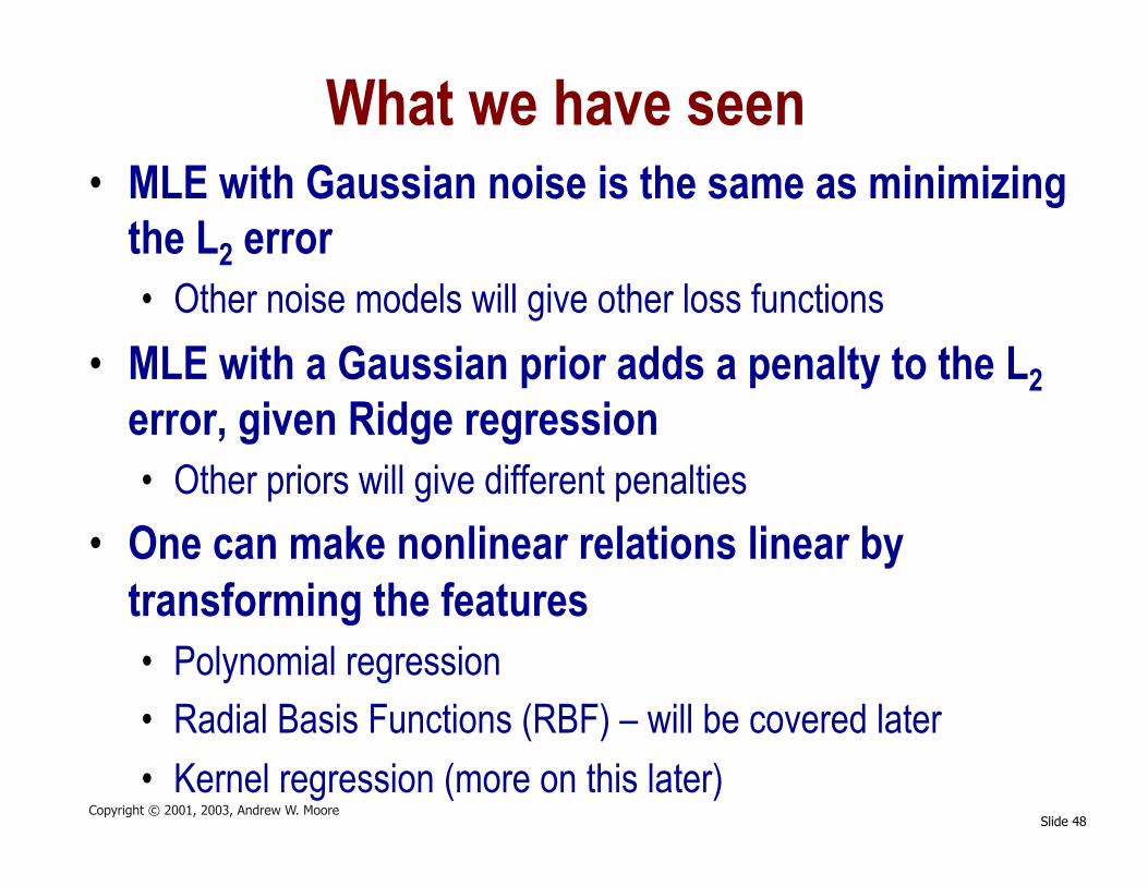
What we have seen • MLE with Gaussian noise is the same as minimizing
the L2 error • Other noise models will give other loss functions
• MLE with a Gaussian prior adds a penalty to the L2 error, given Ridge regression • Other priors will give different penalties
• One can make nonlinear relations linear by transforming the features • Polynomial regression • Radial Basis Functions (RBF) – will be covered later • Kernel regression (more on this later)
Copyright © 2001, 2003, Andrew W. Moore