Lincoln Greenhill - National Radio Astronomy Observatory · VHF . Brogan et al. 2006 330 MHz...
63
Thirteenth Synthesis Imaging Workshop 2012 May 29– June 5 Low-frequency Interferometry Lincoln Greenhill
Transcript of Lincoln Greenhill - National Radio Astronomy Observatory · VHF . Brogan et al. 2006 330 MHz...
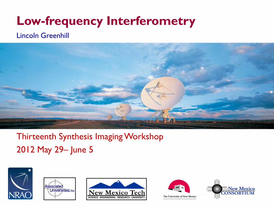
Thirteenth Synthesis Imaging Workshop
2012 May 29– June 5
Low-frequency Interferometry Lincoln Greenhill
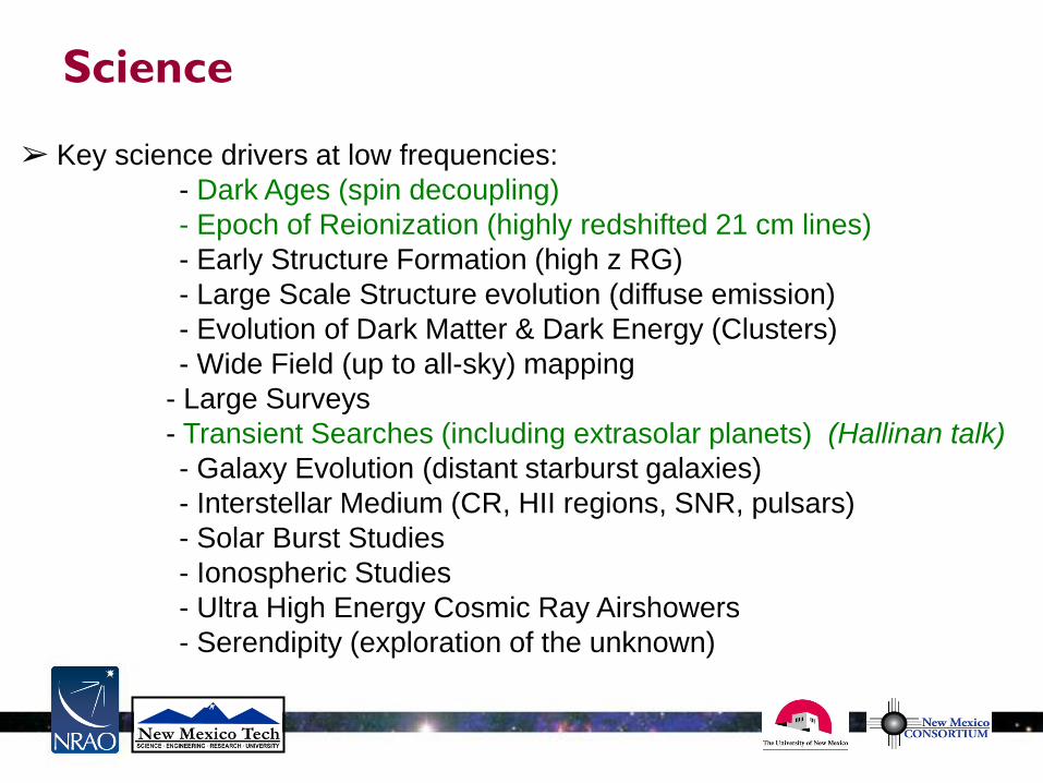
➢ Key science drivers at low frequencies:
- Dark Ages (spin decoupling)
- Epoch of Reionization (highly redshifted 21 cm lines)
- Early Structure Formation (high z RG)
- Large Scale Structure evolution (diffuse emission)
- Evolution of Dark Matter & Dark Energy (Clusters)
- Wide Field (up to all-sky) mapping
- Large Surveys
- Transient Searches (including extrasolar planets) (Hallinan talk)
- Galaxy Evolution (distant starburst galaxies)
- Interstellar Medium (CR, HII regions, SNR, pulsars)
- Solar Burst Studies
- Ionospheric Studies
- Ultra High Energy Cosmic Ray Airshowers
- Serendipity (exploration of the unknown)
Science
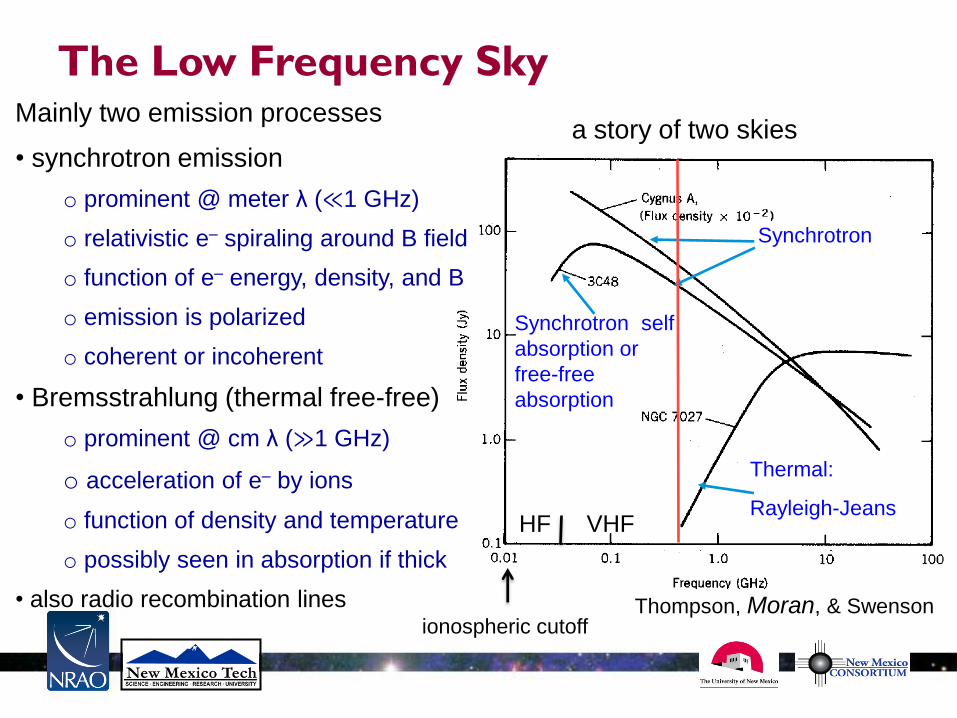
Synchrotron self
absorption or
free-free
absorption
Thermal:
Rayleigh-Jeans
Synchrotron
Mainly two emission processes
• synchrotron emission
o prominent @ meter λ (≪1 GHz)
o relativistic e– spiraling around B field
o function of e– energy, density, and B
o emission is polarized
o coherent or incoherent
• Bremsstrahlung (thermal free-free)
o prominent @ cm λ (≫1 GHz)
o acceleration of e– by ions
o function of density and temperature
o possibly seen in absorption if thick
• also radio recombination lines Thompson, Moran, & Swenson
The Low Frequency Sky
a story of two skies
HF
ionospheric cutoff
VHF
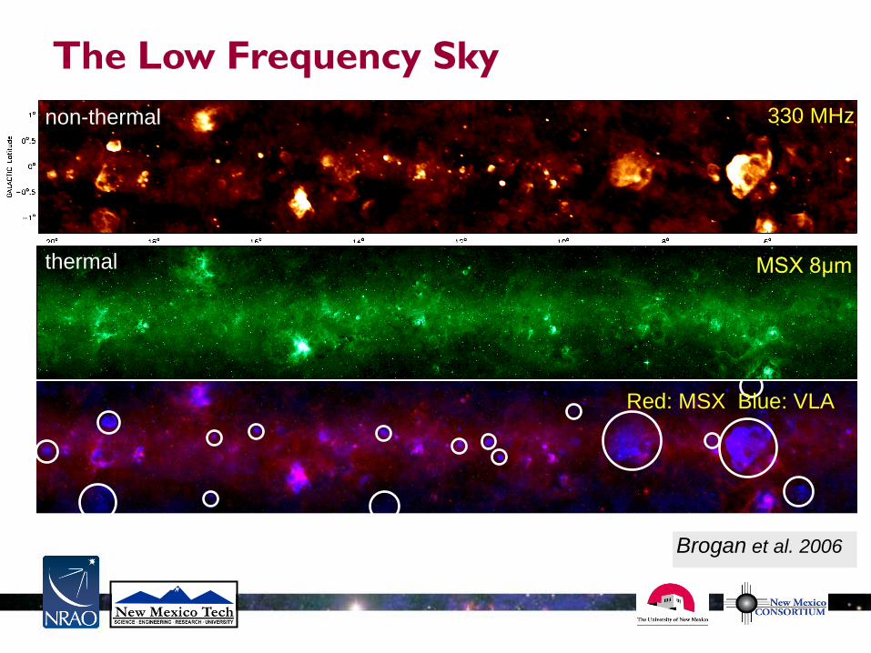
Brogan et al. 2006
330 MHz
8 m MSX 8μm thermal
non-thermal
The Low Frequency Sky
Red: MSX Blue: VLA
Thirteenth Synthesis Imaging Workshop 5
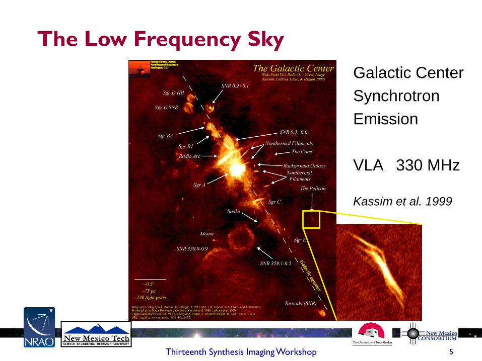
The Low Frequency Sky
Kassim et al. 1999
Galactic Center
Synchrotron
Emission
VLA 330 MHz
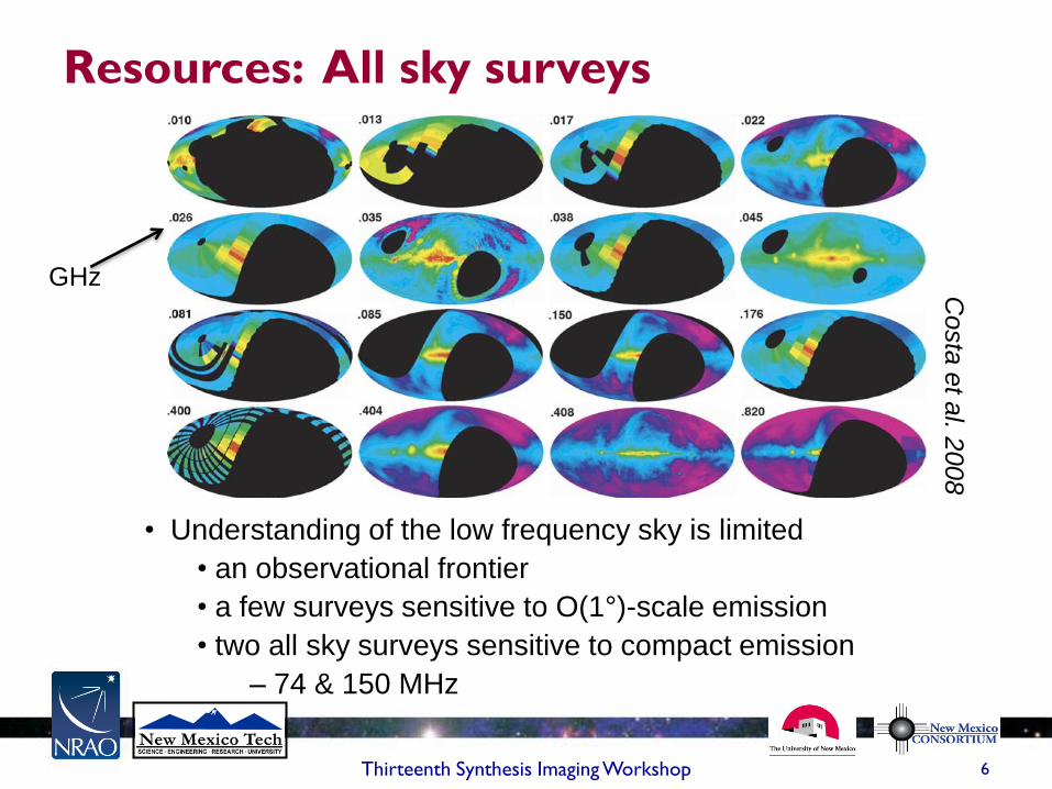
Resources: All sky surveys
Thirteenth Synthesis Imaging Workshop 6
Costa
et a
l. 2008
• Understanding of the low frequency sky is limited
• an observational frontier
• a few surveys sensitive to O(1°)-scale emission
• two all sky surveys sensitive to compact emission
– 74 & 150 MHz
GHz

Resources: VLA Low Frequency Sky Survey
survey parameters: = 74 MHz, > -30°,
= 80″ resolution,
RMS~100 mJy/beam
N ~ 70,000 sources in ~ 95% of sky > -30°
Statistical sample of mundane & rare populations
➟ fast pulsars, distant radio galaxies, cluster radio
halos and relics
calibration grid for low-frequency instruments
data online at NED & http://lwa.nrl.navy.mil/VLSS
successor ELVA low-frequency system in development
10x bandwidth @ 74 MHz
leverages increased correlator capability
Cohen et al. (2007)
19
~20o
VLSS FIELD 1700+690 74 MHz, ~80″, rms ~50 mJy
(Cohen et al. 2007)
Thirteenth Synthesis Imaging Workshop 9
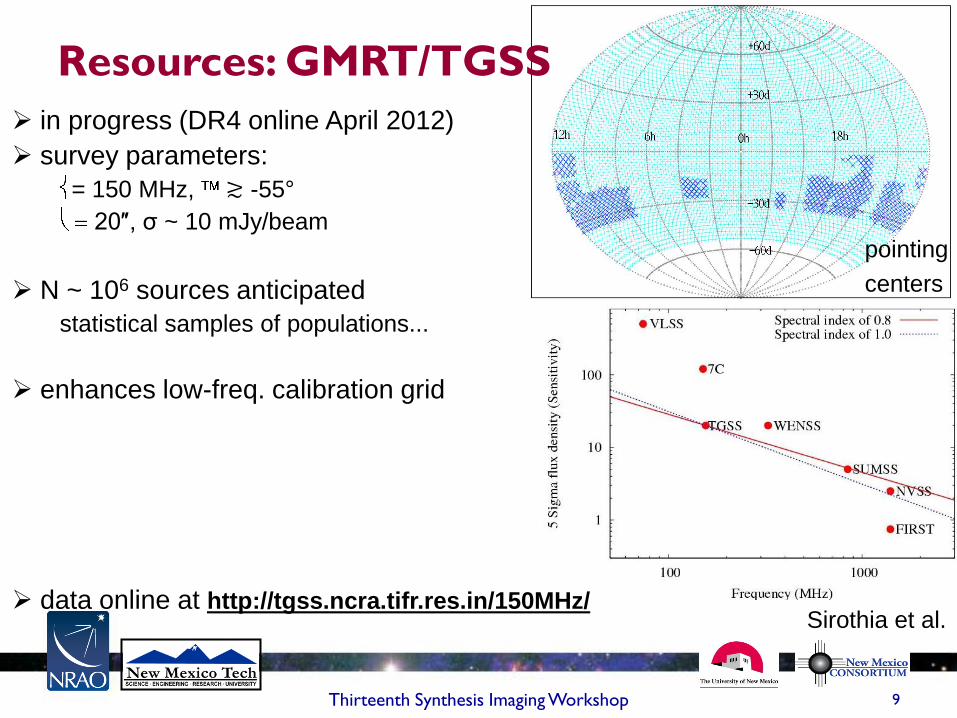
in progress (DR4 online April 2012)
survey parameters:
= 150 MHz, ≳ -55°
20″, σ ~ 10 mJy/beam
N ~ 106 sources anticipated
statistical samples of populations...
enhances low-freq. calibration grid
data online at http://tgss.ncra.tifr.res.in/150MHz/
Resources: GMRT/TGSS
Sirothia et al.
pointing
centers
10 Twelfth Synthesis Imaging Workshop
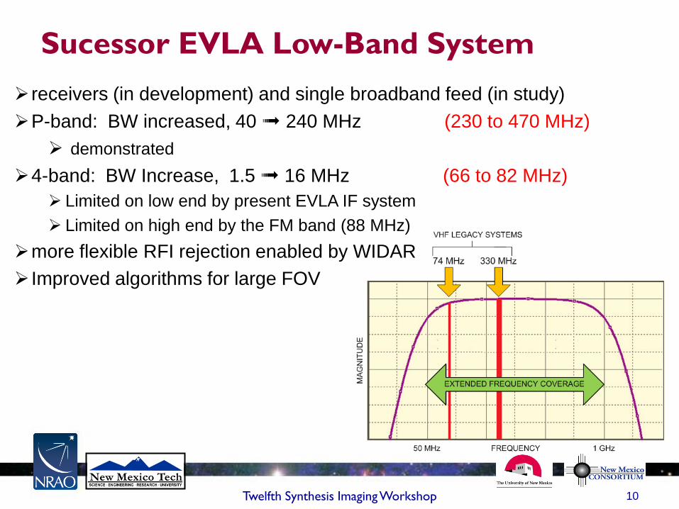
Sucessor EVLA Low-Band System
receivers (in development) and single broadband feed (in study)
P-band: BW increased, 40 ➟ 240 MHz (230 to 470 MHz)
demonstrated
4-band: BW Increase, 1.5 ➟ 16 MHz (66 to 82 MHz)
Limited on low end by present EVLA IF system
Limited on high end by the FM band (88 MHz)
more flexible RFI rejection enabled by WIDAR
Improved algorithms for large FOV
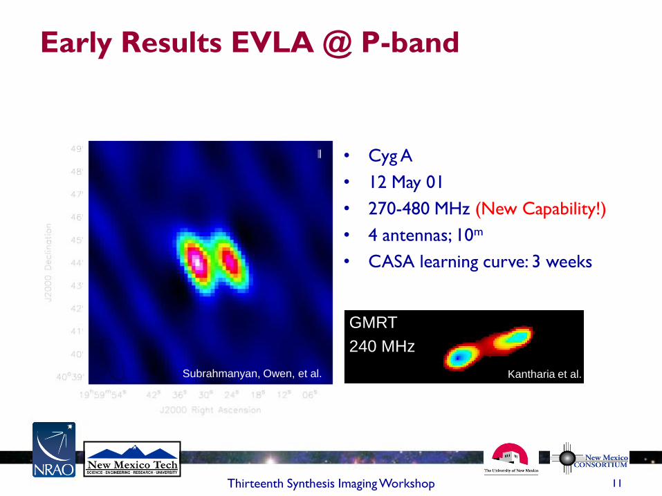
• Cyg A
• 12 May 01
• 270-480 MHz (New Capability!)
• 4 antennas; 10m
• CASA learning curve: 3 weeks
Early Results EVLA @ P-band
Thirteenth Synthesis Imaging Workshop 11
GMRT
240 MHz
Kantharia et al. Subrahmanyan, Owen, et al.
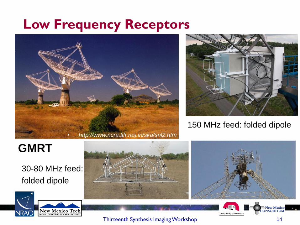
Low Frequency Receptors
• feeds (Hayward talk)
– horns at high/mid frequency
• impractical below ~ 1 GHz: size > λ ➟ massive, awkward
– bare dipoles at low frequency
• basic model: λ/2 resonant (narrow-band) antenna
• ‘electrically short’ dipoles are effective
• diversity of space-saving configurations
• BUT broadband designs involve many trade-offs
– messy circuit elements (variable impedance, ugly gain patterns,…)
• two common configurations
– dipole + dish: large collecting area per dipole ($$$)
– dipole + ground screen: small area, Ae ~ Gλ2/4π ($)
• motivates ‘large-N’ arrays or beam forming ⇐ crazy-new architectures
12 Thirteenth Synthesis Imaging Workshop
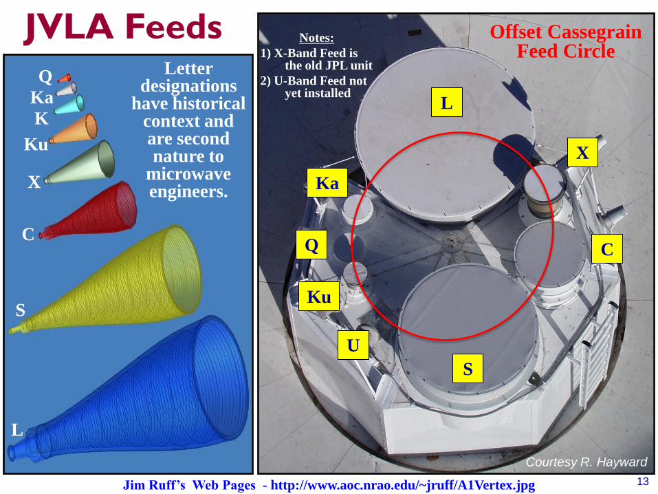
Jim Ruff’s Web Pages - http://www.aoc.nrao.edu/~jruff/A1Vertex.jpg
Notes:
1) X-Band Feed is the old JPL unit
2) U-Band Feed not yet installed
JVLA Feeds
Q
Ka
K
Ku
X
C
S
L
S
L
C
X
Ka
Q
Ku
U
Offset Cassegrain Feed Circle
13
Letter designations
have historical context and are second nature to
microwave engineers.
Courtesy R. Hayward
14 Thirteenth Synthesis Imaging Workshop
GMRT
150 MHz feed: folded dipole
30-80 MHz feed:
folded dipole
Low Frequency Receptors
• http://www.ncra.tifr.res.in/ska/snl2.htm
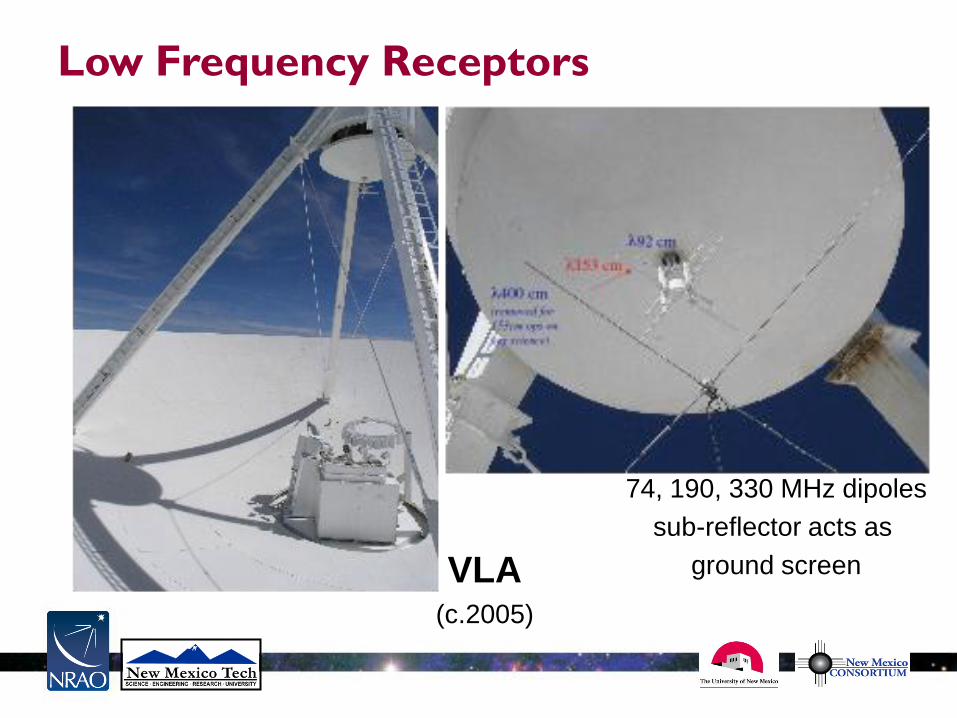
VLA (c.2005)
74, 190, 330 MHz dipoles
sub-reflector acts as
ground screen
Low Frequency Receptors
Thirteenth Synthesis Imaging Workshop 16
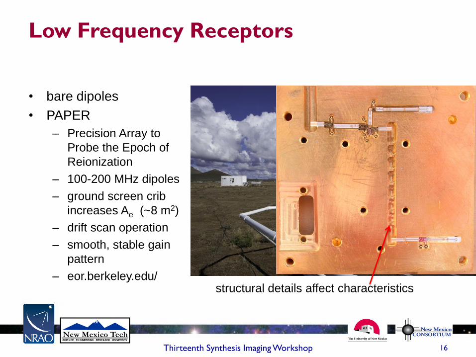
Low Frequency Receptors
• bare dipoles
• PAPER
– Precision Array to
Probe the Epoch of
Reionization
– 100-200 MHz dipoles
– ground screen crib
increases Ae (~8 m2)
– drift scan operation
– smooth, stable gain
pattern
– eor.berkeley.edu/
structural details affect characteristics
17 Thirteenth Synthesis Imaging Workshop
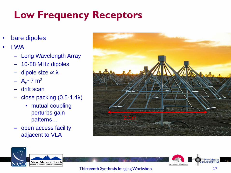
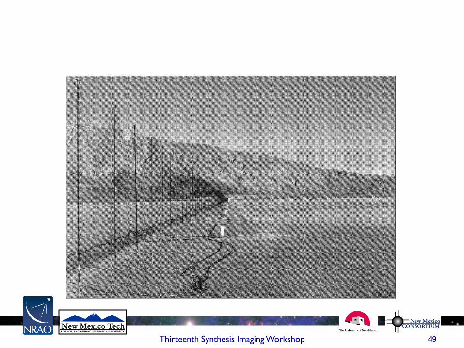
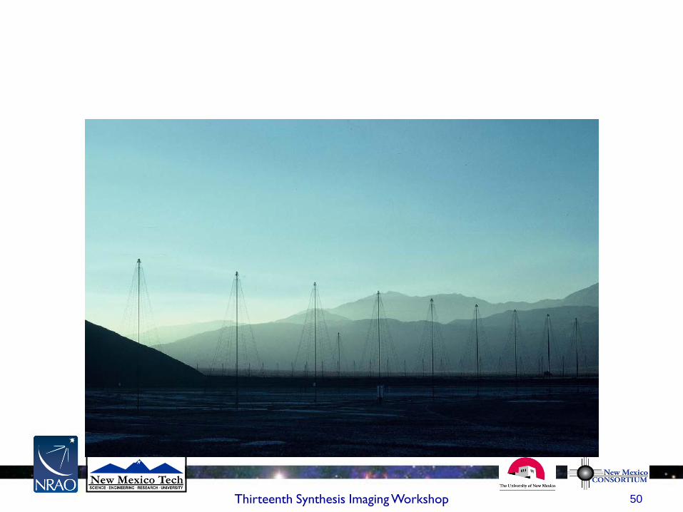
Low Frequency Receptors
• bare dipoles
• LWA
– Long Wavelength Array
– 10-88 MHz dipoles
– dipole size ∝ λ
– Ae~7 m2
– drift scan
– close packing (0.5-1.4λ)
• mutual coupling
perturbs gain
patterns…
– open access facility
adjacent to VLA
2.1m
Thirteenth Synthesis Imaging Workshop 18
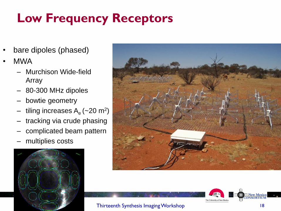
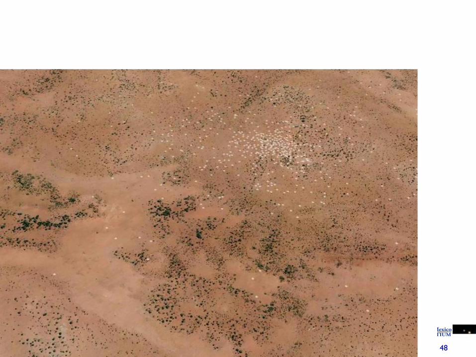
Low Frequency Receptors
• bare dipoles (phased)
• MWA
– Murchison Wide-field
Array
– 80-300 MHz dipoles
– bowtie geometry
– tiling increases Ae (~20 m2)
– tracking via crude phasing
– complicated beam pattern
– multiplies costs
– mwatelescope.org
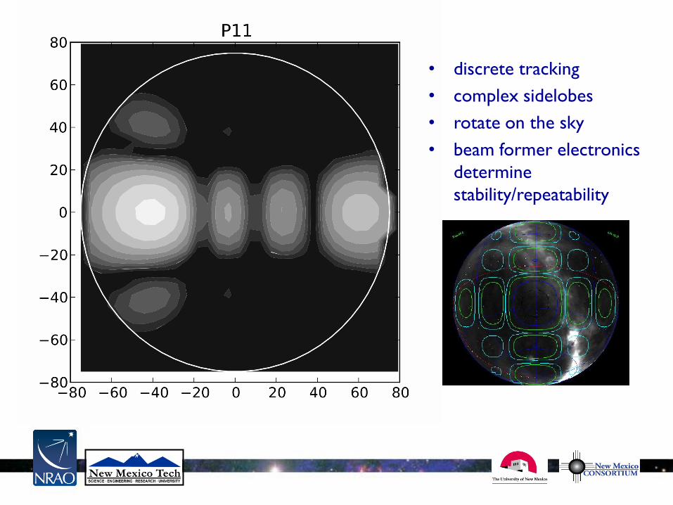
• discrete tracking
• complex sidelobes
• rotate on the sky
• beam former electronics
determine
stability/repeatability
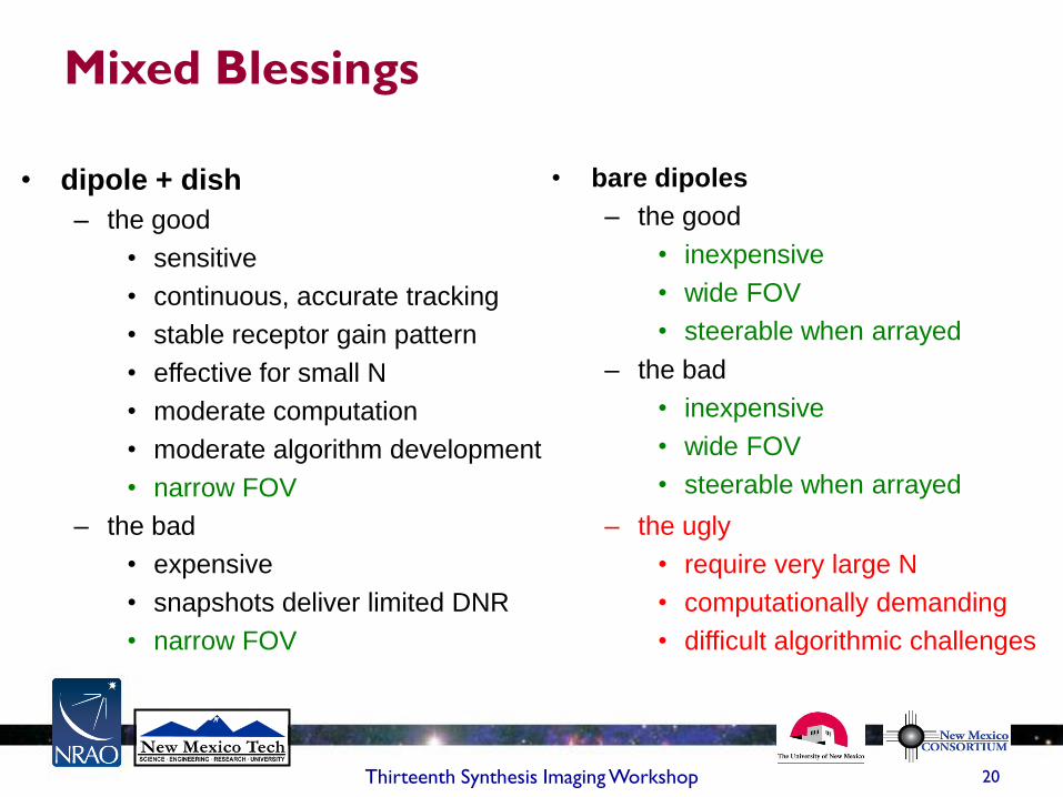
Mixed Blessings
• dipole + dish
– the good
• sensitive
• continuous, accurate tracking
• stable receptor gain pattern
• effective for small N
• moderate computation
• moderate algorithm development
• narrow FOV
– the bad
• expensive
• snapshots deliver limited DNR
• narrow FOV
• bare dipoles
– the good
• inexpensive
• wide FOV
• steerable when arrayed
Thirteenth Synthesis Imaging Workshop 20
– the bad
• inexpensive
• wide FOV
• steerable when arrayed
– the ugly
• require very large N
• computationally demanding
• difficult algorithmic challenges

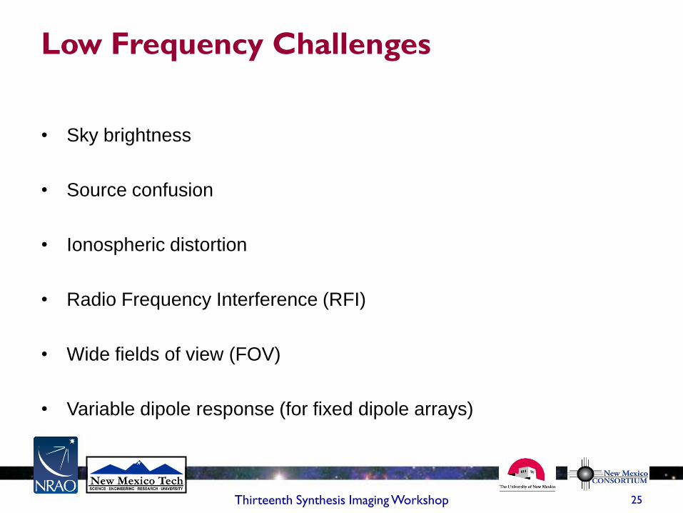
Low Frequency Challenges
• Sky brightness
• Source confusion
• Ionospheric distortion
• Radio Frequency Interference (RFI)
• Wide fields of view (FOV)
• Variable dipole response (for fixed dipole arrays)
Thirteenth Synthesis Imaging Workshop 21

22 Thirteenth Synthesis Imaging Workshop
RFI
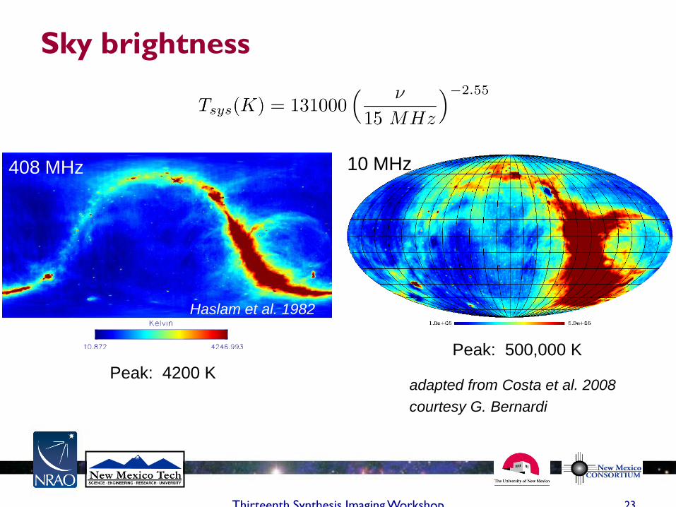
Sky brightness
Thirteenth Synthesis Imaging Workshop 23
408 MHz
Haslam et al. 1982
Peak: 4200 K
10 MHz
adapted from Costa et al. 2008
courtesy G. Bernardi
Peak: 500,000 K
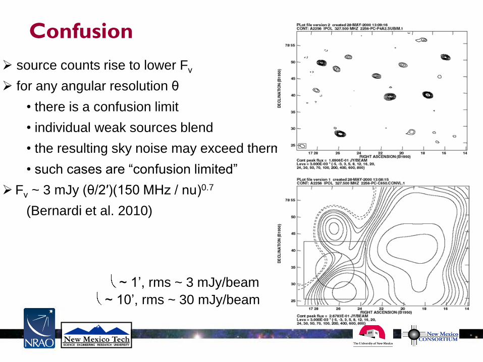
Confusion
source counts rise to lower Fν
for any angular resolution θ
• there is a confusion limit
• individual weak sources blend
• the resulting sky noise may exceed thermal noise
• such cases are “confusion limited”
Fν ~ 3 mJy (θ/2′)(150 MHz / nu)0.7
(Bernardi et al. 2010)
~ 1’, rms ~ 3 mJy/beam
~ 10’, rms ~ 30 mJy/beam
Low Frequency Challenges
• Sky brightness
• Source confusion
• Ionospheric distortion
• Radio Frequency Interference (RFI)
• Wide fields of view (FOV)
• Variable dipole response (for fixed dipole arrays)
Thirteenth Synthesis Imaging Workshop 25
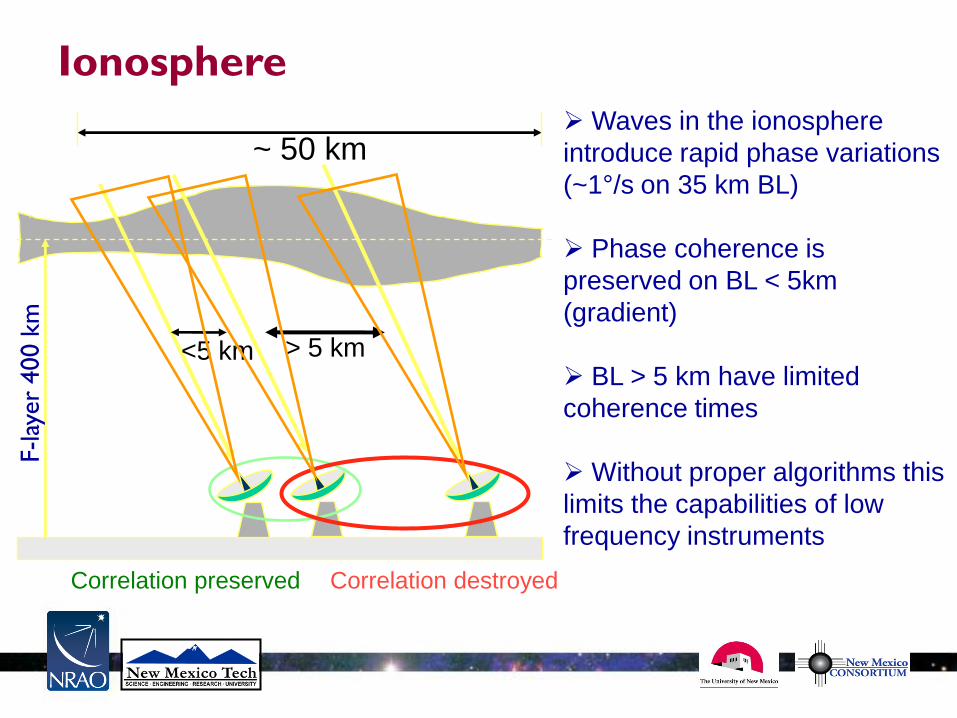
~ 50 km
> 5 km <5 km
Waves in the ionosphere
introduce rapid phase variations
(~1°/s on 35 km BL)
Phase coherence is
preserved on BL < 5km
(gradient)
BL > 5 km have limited
coherence times
Without proper algorithms this
limits the capabilities of low
frequency instruments
Correlation preserved Correlation destroyed
F-lay
er
400 k
m
Ionosphere
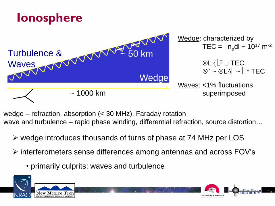
Wedge: characterized by
TEC = nedl ~ 1017 m-2
L 2 TEC
~ L ~ * TEC
Waves: <1% fluctuations
superimposed
wedge introduces thousands of turns of phase at 74 MHz per LOS
interferometers sense differences among antennas and across FOV’s
• primarily culprits: waves and turbulence
Ionosphere
~ 1000 km
Wedge
Turbulence &
Waves ~ 50 km
wedge – refraction, absorption (< 30 MHz), Faraday rotation
wave and turbulence – rapid phase winding, differential refraction, source distortion…
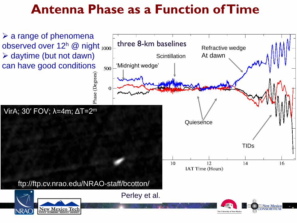
Antenna Phase as a Function of Time
Scintillation
Refractive wedge
At dawn
Quiesence
‘Midnight wedge’
TIDs
VirA; 30′ FOV; λ=4m; ΔT=2m
a range of phenomena
observed over 12h @ night
daytime (but not dawn)
can have good conditions
three 8-km baselines
Perley et al.
ftp://ftp.cv.nrao.edu/NRAO-staff/bcotton/
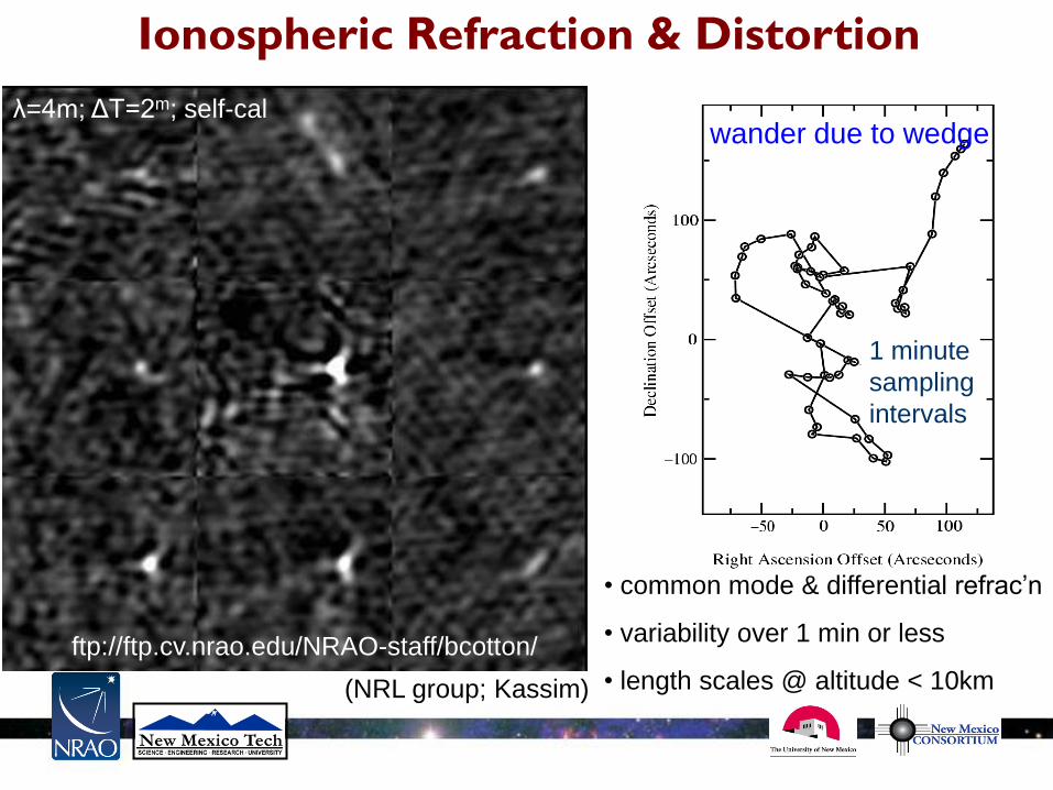
Ionospheric Refraction & Distortion
• common mode & differential refrac’n
• variability over 1 min or less
• length scales @ altitude < 10km
1 minute
sampling
intervals
wander due to wedge
(NRL group; Kassim)
ftp://ftp.cv.nrao.edu/NRAO-staff/bcotton/
λ=4m; ΔT=2m; self-cal
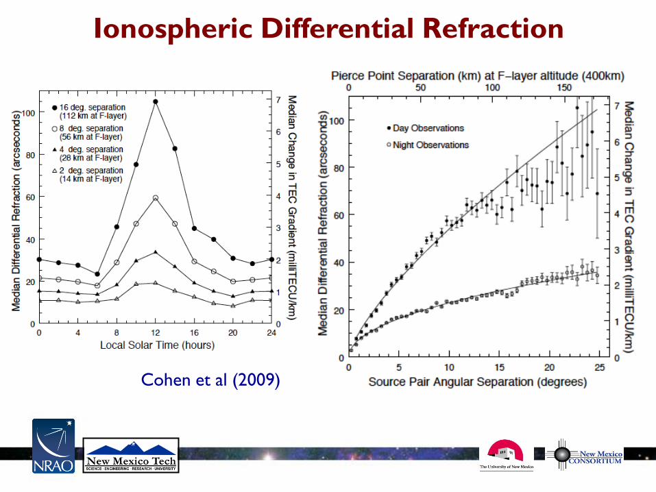
Ionospheric Differential Refraction
Cohen et al (2009)
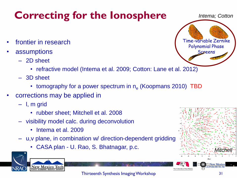
Correcting for the Ionosphere
Thirteenth Synthesis Imaging Workshop 31
• frontier in research
• assumptions
– 2D sheet
• refractive model (Intema et al. 2009; Cotton: Lane et al. 2012)
– 3D sheet
• tomography for a power spectrum in ne (Koopmans 2010) TBD
• corrections may be applied in
– l, m grid
• rubber sheet; Mitchell et al. 2008
– visibility model calc. during deconvolution
• Intema et al. 2009
– u,v plane, in combination w/ direction-dependent gridding
• CASA plan - U. Rao, S. Bhatnagar, p.c. Mitchell
Time-variable Zernike Polynomial Phase
Screens
Intema; Cotton

Low Frequency Challenges
• Sky brightness
• Source confusion
• Ionospheric distortion
• Radio Frequency Interference (RFI)
• Wide fields of view (FOV)
• Variable dipole response (for fixed dipole arrays)
Thirteenth Synthesis Imaging Workshop 32
natural & man-generated RFI at low frequencies is pervasive power lines
broadcast, communications, & radar
digital hardware
keeping sites clean requires care / easily spoiled
at GMRT & LWA: power line noise has been a problem
at VLA: many signatures between 74 and 330 MHz
narrowband, wideband, time varying, ‘wandering’
can be wideband (affecting C & D configurations)
solar effects – unpredictable
quiet sun is a benign 2000 Jy disk at 74 MHz
solar bursts can be 109 Jy and lead to geomagnetic storms
mitigation is done first in a processing path
usually requires high spectral resolution and short time averaging
Radio Frequency Interference
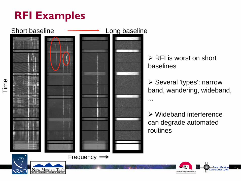
Tim
e
RFI is worst on short
baselines
Several 'types': narrow
band, wandering, wideband,
...
Wideband interference
can degrade automated
routines
Short baseline Long baseline
Frequency
Tim
e
RFI Examples
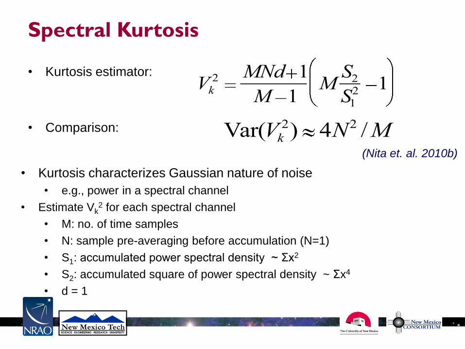
Spectral Kurtosis
• Kurtosis estimator:
• Comparison:
Vk2 MNd 1
M 1MS2S12 1
Var(Vk2) 4N2 /M
(Nita et. al. 2010b)
• Kurtosis characterizes Gaussian nature of noise
• e.g., power in a spectral channel
• Estimate Vk2 for each spectral channel
• M: no. of time samples
• N: sample pre-averaging before accumulation (N=1)
• S1: accumulated power spectral density ~ Σx2
• S2: accumulated square of power spectral density ~ Σx4
• d = 1
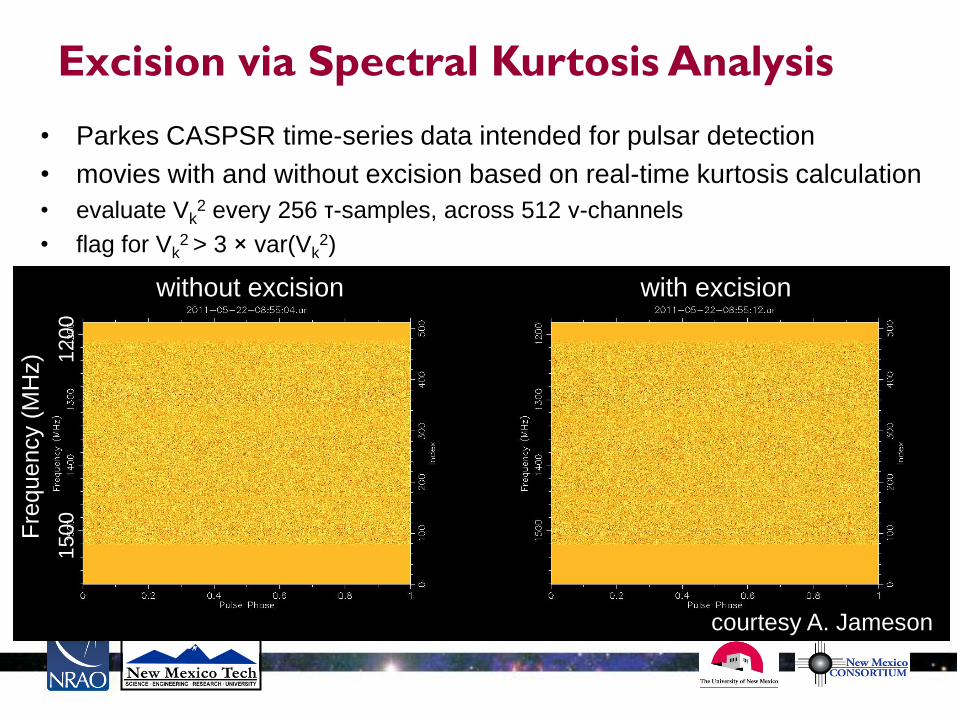
Excision via Spectral Kurtosis Analysis
courtesy A. Jameson
• Parkes CASPSR time-series data intended for pulsar detection
• movies with and without excision based on real-time kurtosis calculation
• evaluate Vk2 every 256 τ-samples, across 512 ν-channels
• flag for Vk2 > 3 × var(Vk
2)
without excision with excision
Fre
quency (
MH
z)
1500
1
200
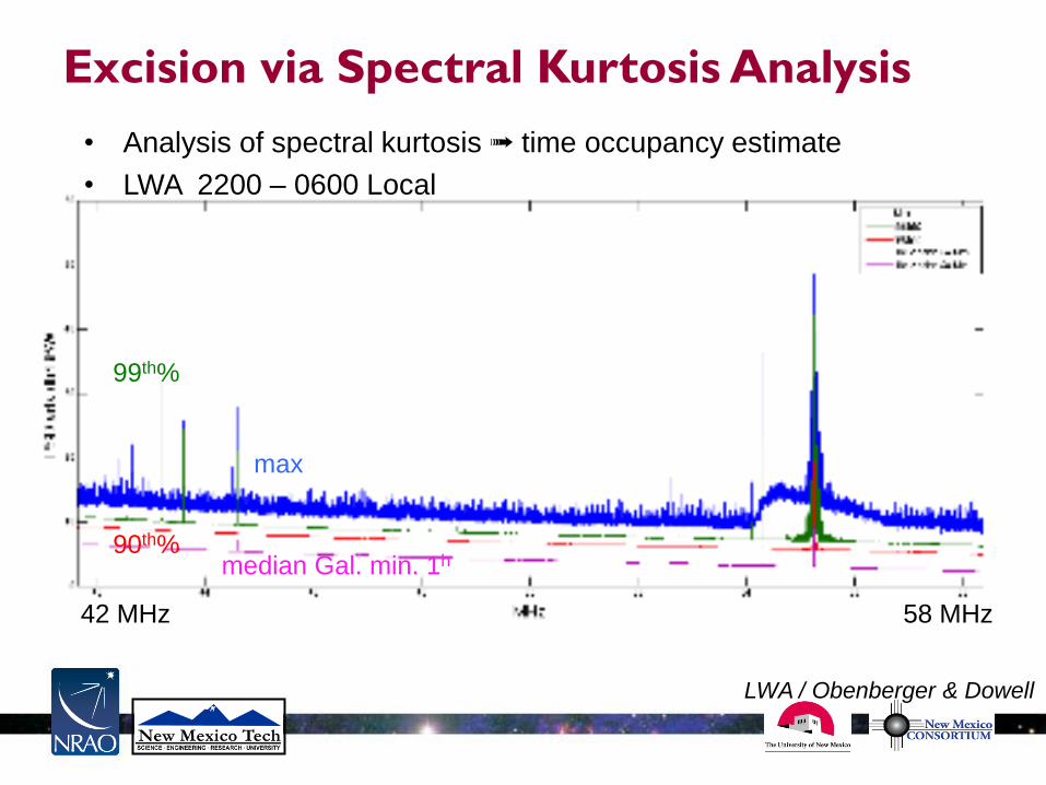
max
99th%
90th% median Gal. min. 1h
42 MHz 58 MHz
LWA / Obenberger & Dowell
• Analysis of spectral kurtosis ➟ time occupancy estimate
• LWA 2200 – 0600 Local
Excision via Spectral Kurtosis Analysis

Low Frequency Challenges
• Sky brightness
• Source confusion
• Ionospheric distortion
• Radio Frequency Interference (RFI)
• Wide fields of view (FOV)
• Variable dipole response (for fixed dipole arrays)
Thirteenth Synthesis Imaging Workshop 38
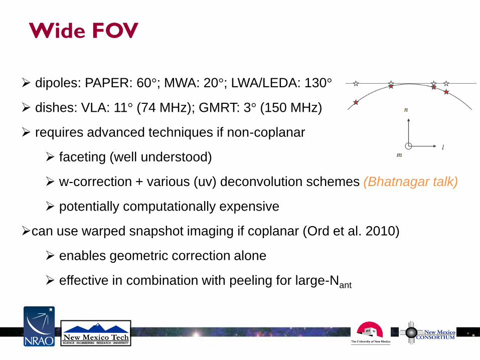
dipoles: PAPER: 60°; MWA: 20°; LWA/LEDA: 130°
dishes: VLA: 11° (74 MHz); GMRT: 3° (150 MHz)
requires advanced techniques if non-coplanar
faceting (well understood)
w-correction + various (uv) deconvolution schemes (Bhatnagar talk)
potentially computationally expensive
can use warped snapshot imaging if coplanar (Ord et al. 2010)
enables geometric correction alone
effective in combination with peeling for large-Nant
Wide FOV
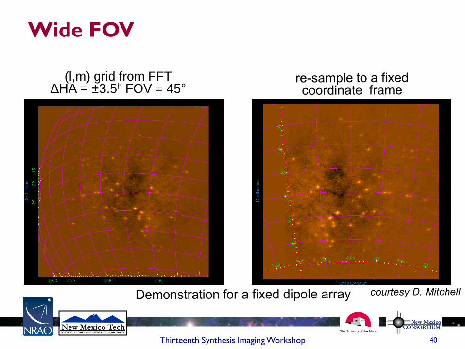
Wide FOV
Thirteenth Synthesis Imaging Workshop 40
(l,m) grid from FFT ΔHA = ±3.5h FOV = 45°
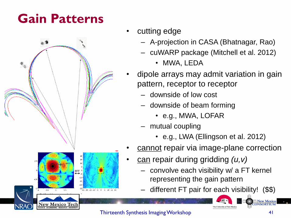
Gain Patterns
Thirteenth Synthesis Imaging Workshop 41
• cutting edge
– A-projection in CASA (Bhatnagar, Rao)
– cuWARP package (Mitchell et al. 2012)
• MWA, LEDA
• dipole arrays may admit variation in gain
pattern, receptor to receptor
– downside of low cost
– downside of beam forming
• e.g., MWA, LOFAR
– mutual coupling
• e.g., LWA (Ellingson et al. 2012)
• cannot repair via image-plane correction
• can repair during gridding (u,v)
– convolve each visibility w/ a FT kernel
representing the gain pattern
– different FT pair for each visibility! ($$)
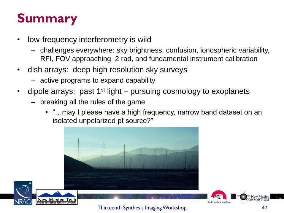
Summary
• low-frequency interferometry is wild
– challenges everywhere: sky brightness, confusion, ionospheric variability,
RFI, FOV approaching 2 rad, and fundamental instrument calibration
• dish arrays: deep high resolution sky surveys
– active programs to expand capability
• dipole arrays: past 1st light – pursuing cosmology to exoplanets
– breaking all the rules of the game
• “…may I please have a high frequency, narrow band dataset on an
isolated unpolarized pt source?”
42 Thirteenth Synthesis Imaging Workshop
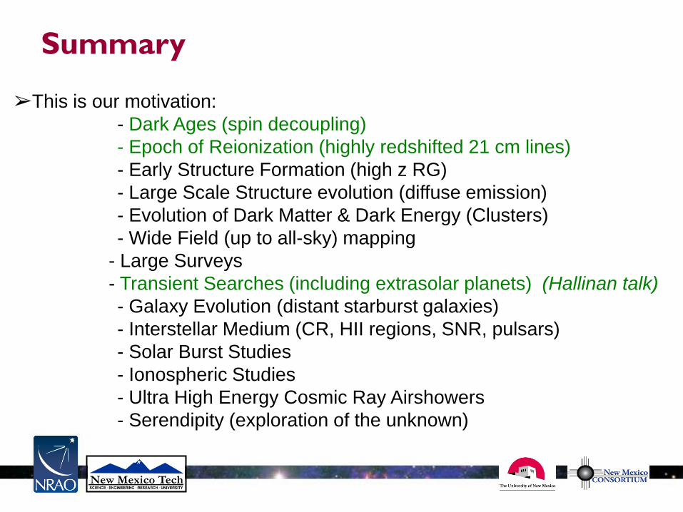
➢This is our motivation:
- Dark Ages (spin decoupling)
- Epoch of Reionization (highly redshifted 21 cm lines)
- Early Structure Formation (high z RG)
- Large Scale Structure evolution (diffuse emission)
- Evolution of Dark Matter & Dark Energy (Clusters)
- Wide Field (up to all-sky) mapping
- Large Surveys
- Transient Searches (including extrasolar planets) (Hallinan talk)
- Galaxy Evolution (distant starburst galaxies)
- Interstellar Medium (CR, HII regions, SNR, pulsars)
- Solar Burst Studies
- Ionospheric Studies
- Ultra High Energy Cosmic Ray Airshowers
- Serendipity (exploration of the unknown)
Summary

44 Thirteenth Synthesis Imaging Workshop

Thirteenth Synthesis Imaging Workshop 45
-end-
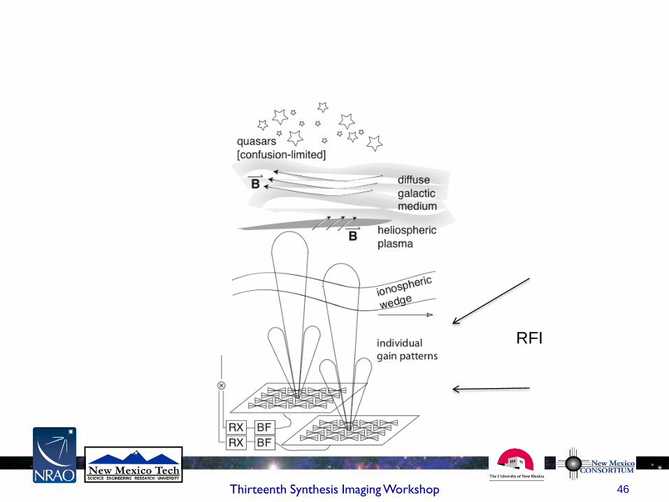
46 Thirteenth Synthesis Imaging Workshop
RFI
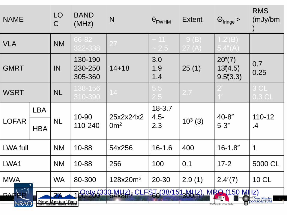
NAME LO
C
BAND
(MHz) N θFWHM Extent Θfringe >
RMS
(mJy/bm
)
VLA NM 66-82
322-338 27
~ 11
~ 2.5
9 (B)
27 (A)
1.2′(B)
5.4″(A)
GMRT IN
130-190
230-250
305-360
14+18
3.0
1.9
1.4
25 (1)
20″ (7′)
13″(4.5′)
9.5″(3.3′)
0.7
0.25
WSRT NL 138-156
310-390 14
5.5
2.5 2.7
2′
1′
3 CL
0.3 CL
LOFAR
LBA
NL 10-90
110-240
25x2x24x2
0m2
18-3.7
4.5-
2.3
103 (3) 40-8″
5-3″
110-12
.4 HBA
LWA full NM 10-88 54x256 16-1.6 400 16-1.8″ 1
LWA1 NM 10-88 256 100 0.1 17-2 5000 CL
MWA WA 80-300 128x20m2 20-30 2.9 (1) 2.4′ (7′) 10 CL
PAPER ZA 100-200 64x8m2 60 300m – – Ooty (330 MHz), CLFST (38/151 MHz), MRO (150 MHz)
Thirteenth Synthesis Imaging Workshop 48
49 Thirteenth Synthesis Imaging Workshop
50 Thirteenth Synthesis Imaging Workshop

51 Thirteenth Synthesis Imaging Workshop

52 Thirteenth Synthesis Imaging Workshop

53 Thirteenth Synthesis Imaging Workshop

54 Thirteenth Synthesis Imaging Workshop

55 Thirteenth Synthesis Imaging Workshop

56 Thirteenth Synthesis Imaging Workshop
57 Thirteenth Synthesis Imaging Workshop
Thirteenth Synthesis Imaging Workshop 58
Thirteenth Synthesis Imaging Workshop 59
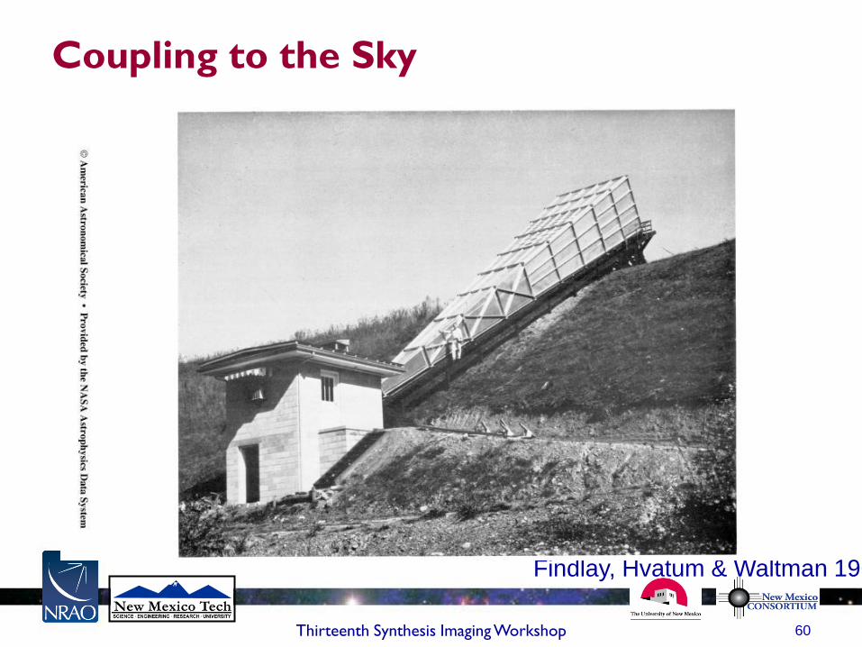
Coupling to the Sky
60 Thirteenth Synthesis Imaging Workshop
Findlay, Hvatum & Waltman 1965
61 Thirteenth Synthesis Imaging Workshop
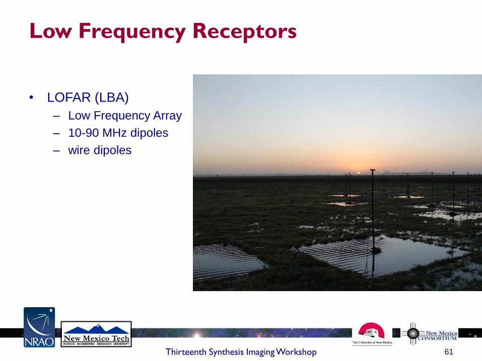
Low Frequency Receptors
• LOFAR (LBA)
– Low Frequency Array
– 10-90 MHz dipoles
– wire dipoles
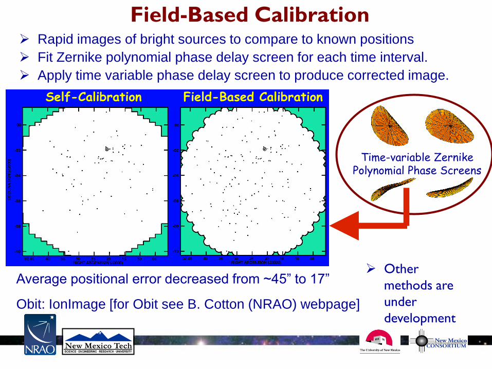
Field-Based Calibration
Average positional error decreased from ~45” to 17”
Obit: IonImage [for Obit see B. Cotton (NRAO) webpage]
Self-Calibration Field-Based Calibration
Time-variable Zernike Polynomial Phase Screens
Rapid images of bright sources to compare to known positions
Fit Zernike polynomial phase delay screen for each time interval.
Apply time variable phase delay screen to produce corrected image.
Other
methods are
under
development
Currently in a transition of moving to high resolution at low frequencies
Why has this taken nearly 50 years?
Software/Computing:
- Ionospheric decorrelation on baselines > 5 km is overcome by software
advances of Self-Calibration in the 1980’s
- Wide-field imaging only recently (sort of) possible
- RFI excision development
- Data transmission from long distances became feasible using fiber-optic
transmission lines
Overcoming the Resolution Problem