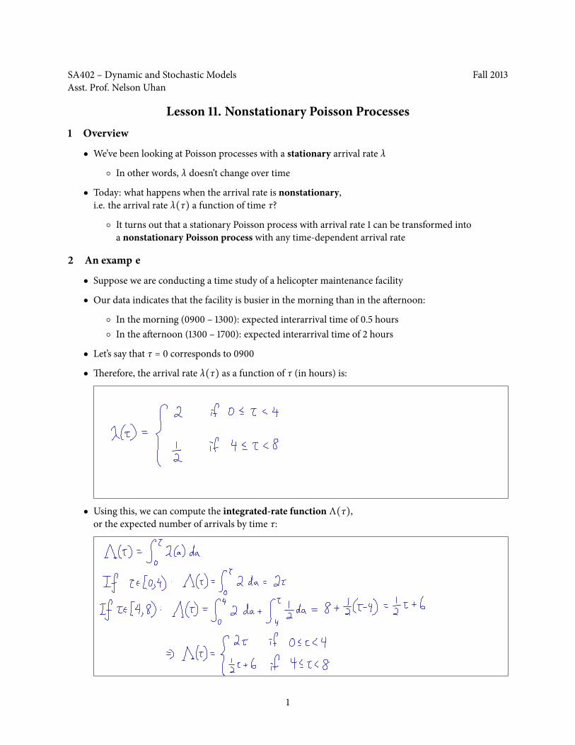
SA402 – Dynamic and Stochastic Models Fall 2013Asst. Prof. Nelson Uhan

Lesson 11. Nonstationary Poisson Processes1 Overview

● We’ve been looking at Poisson processes with a stationary arrival rate λ

○ In other words, λ doesn’t change over time

● Today: what happens when the arrival rate is nonstationary,i.e. the arrival rate λ(τ) a function of time τ?

○ It turns out that a stationary Poisson process with arrival rate 1 can be transformed intoa nonstationary Poisson process with any time-dependent arrival rate

2 An example

● Suppose we are conducting a time study of a helicopter maintenance facility

● Our data indicates that the facility is busier in the morning than in the a&ernoon:

○ In the morning (0900 – 1300): expected interarrival time of 0.5 hours○ In the a&ernoon (1300 – 1700): expected interarrival time of 2 hours

● Let’s say that τ = 0 corresponds to 0900● !erefore, the arrival rate λ(τ) as a function of τ (in hours) is:

● Using this, we can compute the integrated-rate function Λ(τ),or the expected number of arrivals by time τ:

1

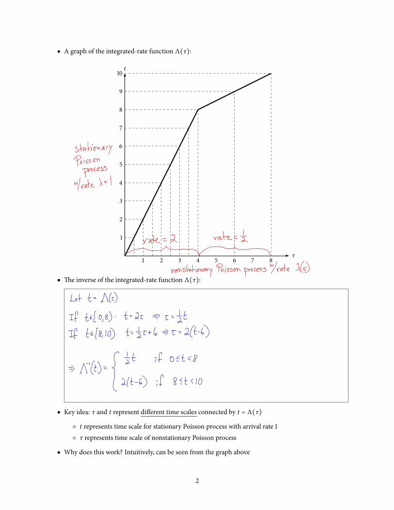
● A graph of the integrated-rate function Λ(τ):

τ

t

1

2

3

4

5

6

7

8

9

10

1 2 3 4 5 6 7 8

● !e inverse of the integrated-rate function Λ(τ):

● Key idea: τ and t represent different time scales connected by t = Λ(τ)○ t represents time scale for stationary Poisson process with arrival rate 1○ τ represents time scale of nonstationary Poisson process

● Why does this work? Intuitively, can be seen from the graph above

2

3 Nonstationary Poisson processes, formally

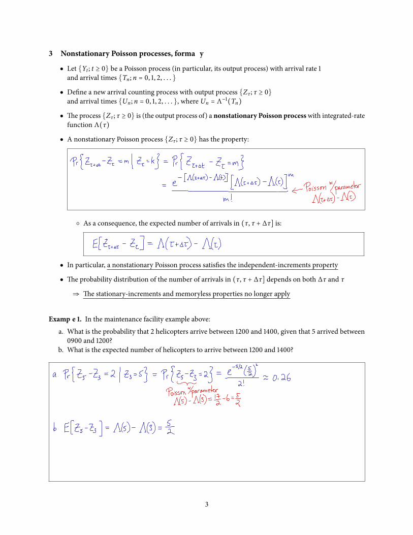
● Let {Yt ; t ≥ 0} be a Poisson process (in particular, its output process) with arrival rate 1and arrival times {Tn; n = 0, 1, 2, . . . }● De$ne a new arrival counting process with output process {Zτ ; τ ≥ 0}and arrival times {Un; n = 0, 1, 2, . . . }, where Un = Λ−1(Tn)● !e process {Zτ ; τ ≥ 0} is (the output process of) a nonstationary Poisson processwith integrated-ratefunction Λ(τ)● A nonstationary Poisson process {Zτ ; τ ≥ 0} has the property:

○ As a consequence, the expected number of arrivals in (τ, τ + ∆τ] is:

● In particular, a nonstationary Poisson process satis$es the independent-increments property

● !e probability distribution of the number of arrivals in (τ, τ + ∆τ] depends on both ∆τ and τ

⇒ !e stationary-increments and memoryless properties no longer apply

Example 1. In the maintenance facility example above:

a. What is the probability that 2 helicopters arrive between 1200 and 1400, given that 5 arrived between0900 and 1200?

b. What is the expected number of helicopters to arrive between 1200 and 1400?

3

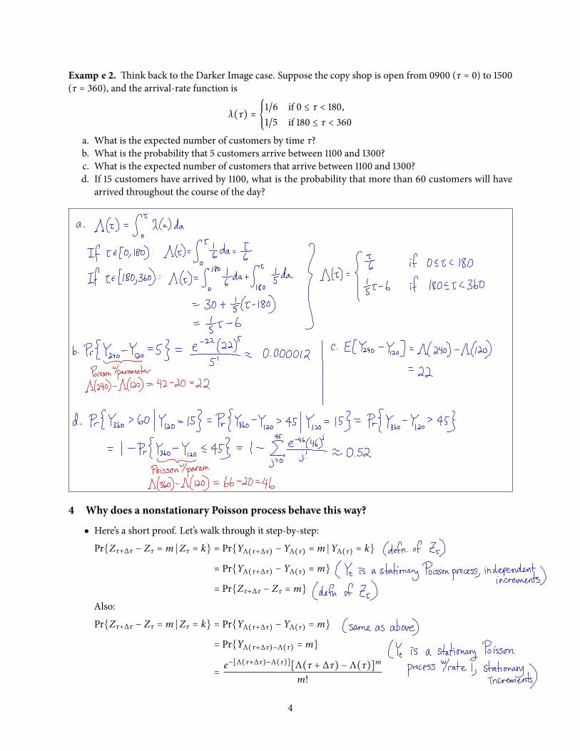
Example 2. !ink back to the Darker Image case. Suppose the copy shop is open from 0900 (τ = 0) to 1500(τ = 360), and the arrival-rate function is

λ(τ) = ⎧⎪⎪⎨⎪⎪⎩1/6 if 0 ≤ τ < 180,1/5 if 180 ≤ τ < 360

a. What is the expected number of customers by time τ?b. What is the probability that 5 customers arrive between 1100 and 1300?c. What is the expected number of customers that arrive between 1100 and 1300?d. If 15 customers have arrived by 1100, what is the probability that more than 60 customers will have

arrived throughout the course of the day?

4 Why does a nonstationary Poisson process behave this way?

● Here’s a short proof. Let’s walk through it step-by-step:

Pr{Zτ+∆τ − Zτ = m ∣ Zτ = k} = Pr{YΛ(τ+∆τ) − YΛ(τ) = m ∣YΛ(τ) = k}= Pr{YΛ(τ+∆τ) − YΛ(τ) = m}= Pr{Zτ+∆τ − Zτ = m}

Also:

Pr{Zτ+∆τ − Zτ = m ∣ Zτ = k} = Pr{YΛ(τ+∆τ) − YΛ(τ) = m}= Pr{YΛ(τ+∆τ)−Λ(τ) = m}= e−[Λ(τ+∆τ)−Λ(τ)][Λ(τ + ∆τ) − Λ(τ)]m

m!

4