Lesson 5 FatigueLow Cycle Fatigue: Plasticizing caused by high stresses applied generates a...
73
Comportamiento Mecánico de Materiales, 3º ICCP Lección 6 LESSON 5 FATIGUE OF MATERIALS
Transcript of Lesson 5 FatigueLow Cycle Fatigue: Plasticizing caused by high stresses applied generates a...
Com
port
amie
nto
Mec
ánic
o de
Mat
eria
les,
3º I
CC
P Le
cció
n 6
LESSON 5
FATIGUE OF MATERIALS
Com
port
amie
nto
Mec
ánic
o de
Mat
eria
les,
3º I
CC
P Le
cció
n 6
INDEX:
6.1. INTRODUCTION
6.2 CYCLIC LOADS
6.3 TOTAL FATIGUE LIFE
6.4 S-N CURVES
6.5 ε-N CURVES
6.6 GLOBAL APPROACH
6.7 FATIGUE CRACK GROWTH
6.8 DETERMINATION OF PARIS LAW
6.9 FACTORS INFLUENCING THE PROPAGATION
6.10 FATIGUE MICROMECHANISM
6.11 FATIGUE DESIGN
Com
port
amie
nto
Mec
ánic
o de
Mat
eria
les,
3º I
CC
P Le
cció
n 6
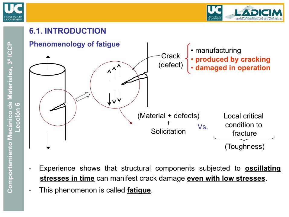
Phenomenology of fatigue
6.1. INTRODUCTION
Crack (defect)
• manufacturing • produced by cracking • damaged in operation
Local critical condition to
fracture
(Toughness)
Vs. (Material + defects)
+ Solicitation
• Experience shows that structural components subjected to oscillating stresses in time can manifest crack damage even with low stresses.
• This phenomenon is called fatigue.
Com
port
amie
nto
Mec
ánic
o de
Mat
eria
les,
3º I
CC
P Le
cció
n 6
Historical examples:
6.1. INTRODUCTION
• LIBERTY SHIPS (1943) • ACCIDENT OF ALOHA AIRLINES FLIGHT B-737 (1988) • ACCIDENT OF THE PRESTIGE (2002) • ALEXANDER KIELLAND DECK COLLAPSE (1980)
Com
port
amie
nto
Mec
ánic
o de
Mat
eria
les,
3º I
CC
P Le
cció
n 6
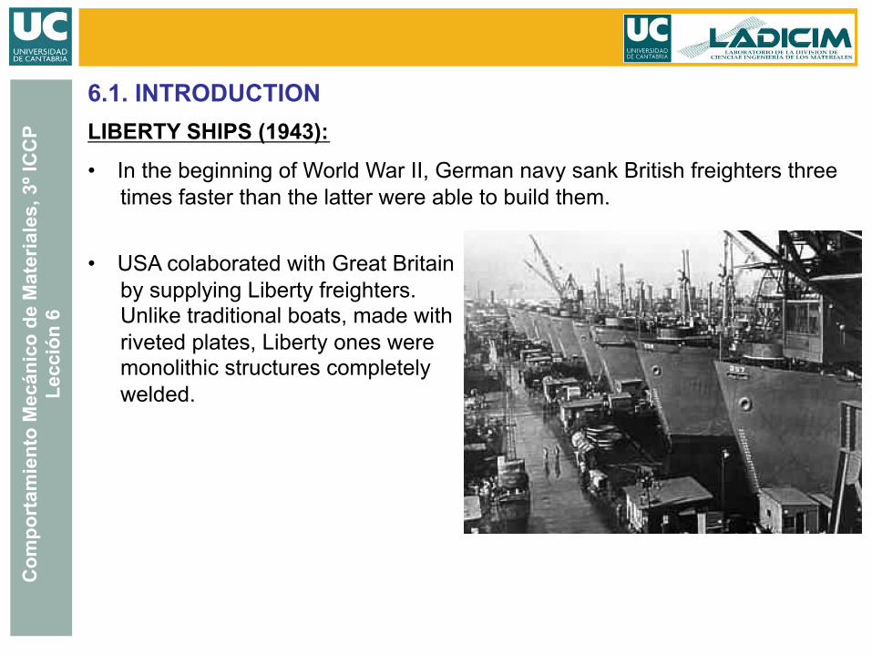
LIBERTY SHIPS (1943):
• In the beginning of World War II, German navy sank British freighters three times faster than the latter were able to build them.
• USA colaborated with Great Britain by supplying Liberty freighters. Unlike traditional boats, made with riveted plates, Liberty ones were monolithic structures completely welded.
6.1. INTRODUCTION
Com
port
amie
nto
Mec
ánic
o de
Mat
eria
les,
3º I
CC
P Le
cció
n 6
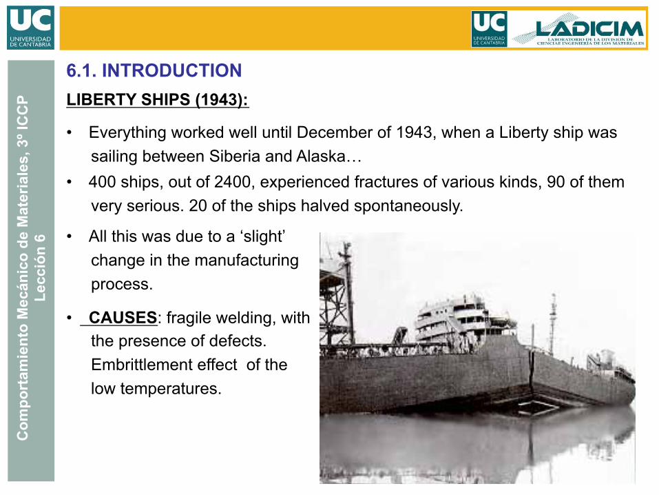
LIBERTY SHIPS (1943):
• Everything worked well until December of 1943, when a Liberty ship was sailing between Siberia and Alaska…
• 400 ships, out of 2400, experienced fractures of various kinds, 90 of them very serious. 20 of the ships halved spontaneously.
• All this was due to a ‘slight’ change in the manufacturing process.
• CAUSES: fragile welding, with the presence of defects. Embrittlement effect of the low temperatures.
6.1. INTRODUCTION
Com
port
amie
nto
Mec
ánic
o de
Mat
eria
les,
3º I
CC
P Le
cció
n 6
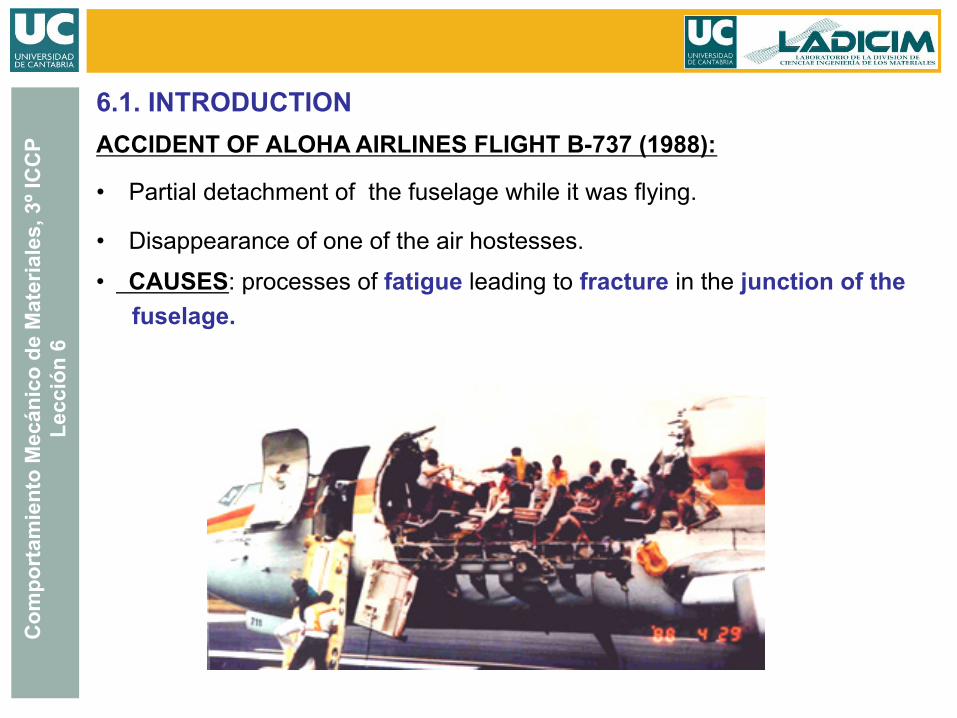
ACCIDENT OF ALOHA AIRLINES FLIGHT B-737 (1988):
• Partial detachment of the fuselage while it was flying.
• Disappearance of one of the air hostesses.
• CAUSES: processes of fatigue leading to fracture in the junction of the fuselage.
6.1. INTRODUCTION
Com
port
amie
nto
Mec
ánic
o de
Mat
eria
les,
3º I
CC
P Le
cció
n 6
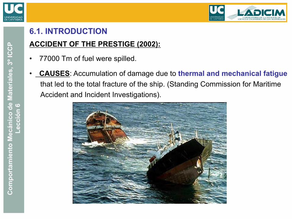
ACCIDENT OF THE PRESTIGE (2002):
• 77000 Tm of fuel were spilled.
• CAUSES: Accumulation of damage due to thermal and mechanical fatigue that led to the total fracture of the ship. (Standing Commission for Maritime Accident and Incident Investigations).
6.1. INTRODUCTION
Com
port
amie
nto
Mec
ánic
o de
Mat
eria
les,
3º I
CC
P Le
cció
n 6
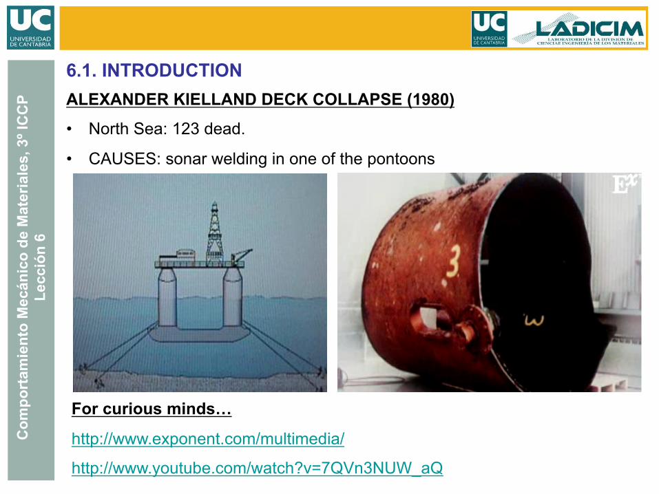
ALEXANDER KIELLAND DECK COLLAPSE (1980)
• North Sea: 123 dead.
• CAUSES: sonar welding in one of the pontoons
For curious minds…
http://www.exponent.com/multimedia/
http://www.youtube.com/watch?v=7QVn3NUW_aQ
6.1. INTRODUCTION
Com
port
amie
nto
Mec
ánic
o de
Mat
eria
les,
3º I
CC
P Le
cció
n 6
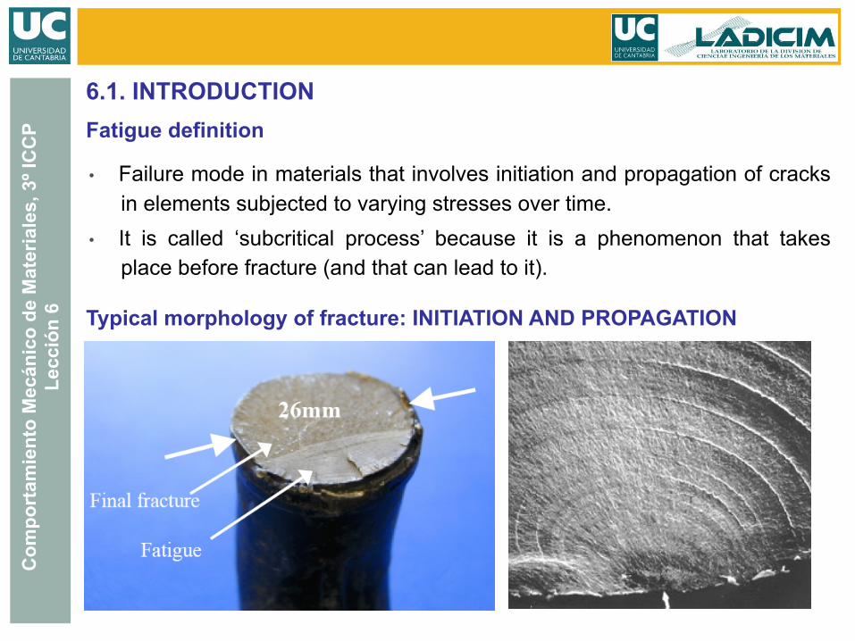
• Failure mode in materials that involves initiation and propagation of cracks in elements subjected to varying stresses over time.
• It is called ‘subcritical process’ because it is a phenomenon that takes place before fracture (and that can lead to it).
Fatigue definition
6.1. INTRODUCTION
Typical morphology of fracture: INITIATION AND PROPAGATION
Com
port
amie
nto
Mec
ánic
o de
Mat
eria
les,
3º I
CC
P Le
cció
n 6
19th Century: Early scientific studies
ALBERT (1829), fatigue tests on iron chains.
PONCELET (1829) AND RANKINE (1843), WÖHLER (1850-1870), breakage of train rails after many cycles with low stress.
20th Century: Emergence of MF and application of fatigue
OROWAN and TAYLOR (1930) develop dislocation concept.
GRIFFITH (1921) and IRWIN (since 1950) lay the foundations of FM.
PARIS (1961): application of FM to fatigue processes.
Other authors: extension to various materials and structural situations.
6.1. INTRODUCTION
Com
port
amie
nto
Mec
ánic
o de
Mat
eria
les,
3º I
CC
P Le
cció
n 6
KEY IDEAS: 6.1. INTRODUCTION
• Monotonous loads do not produce fatigue damage. They must be oscillating over time.
• It has been estimated that the costs associated with fracture of components and structures in the U.S.A. account for a 4% of the GDP.
• There have been thousands of accidents, sometimes with fatal consequences.
• Currently there is a characterization and analysis tool available that spot fatigue in both design of components stage and inspection and performance assessment.
• 20th and 21st Centuries: Fatigue design codes of structural elements and components. Eg: Eurocode, ASME, API, FITNET…
Com
port
amie
nto
Mec
ánic
o de
Mat
eria
les,
3º I
CC
P Le
cció
n 6
The fatigue life evaluation can be done from two perspectives:
1) Estimation of the total life of the element (initiation + propagation). It has its origin in the studies of Wöhler, Basquin and Goodman (19th Century), and it is based on experimental and statistical studies. The design parameter is the endurance.
2) Evaluation of the component life through propagation, assuming the existence of certain size cracks. This perspective starts with FM and Paris work (60’s).
6.1. INTRODUCTION GENERAL SCHEME:
Com
port
amie
nto
Mec
ánic
o de
Mat
eria
les,
3º I
CC
P Le
cció
n 6
6.1. INTRODUCTION
INTRINSIC PROBLEMS IN THE FATIGUE ANALYSIS:
1) Laboratory results show that it is a random phenomenon and, therefore, difficult to predict: identical specimens tested under similar conditions manifest different fatigue behaviors. Different probability distributions have been used to model the random behavior of fatigue: normal distribution, extreme values, Birnbaum-Sanders or Weibull.
2) It is difficult translate experimental results to real situations.
3) In many cases, it is impossible to know beforehand the operation conditions of the component (eg, wind, waves…).
4) The same can be said about environmental conditions; furthermore, they normally generate difficult synergetic mechanisms (impossible?) to evaluate / predict.
Com
port
amie
nto
Mec
ánic
o de
Mat
eria
les,
3º I
CC
P Le
cció
n 6
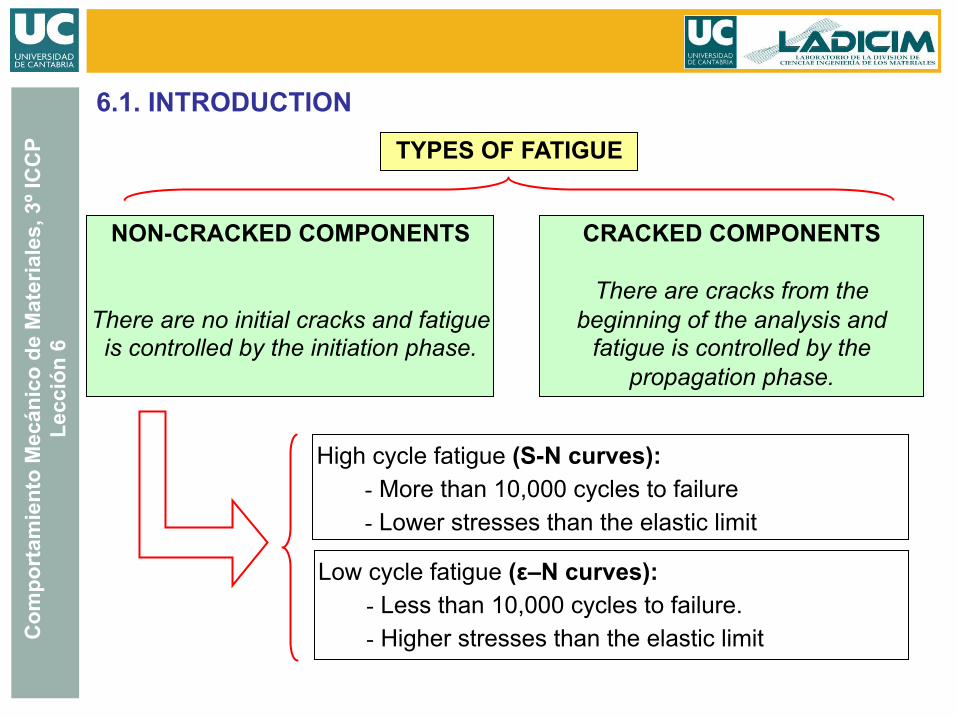
TYPES OF FATIGUE
NON-CRACKED COMPONENTS
There are no initial cracks and fatigue is controlled by the initiation phase.
High cycle fatigue (S-N curves): - More than 10,000 cycles to failure - Lower stresses than the elastic limit
CRACKED COMPONENTS
There are cracks from the beginning of the analysis and
fatigue is controlled by the propagation phase.
Low cycle fatigue (ε–N curves): - Less than 10,000 cycles to failure. - Higher stresses than the elastic limit
6.1. INTRODUCTION
Com
port
amie
nto
Mec
ánic
o de
Mat
eria
les,
3º I
CC
P Le
cció
n 6
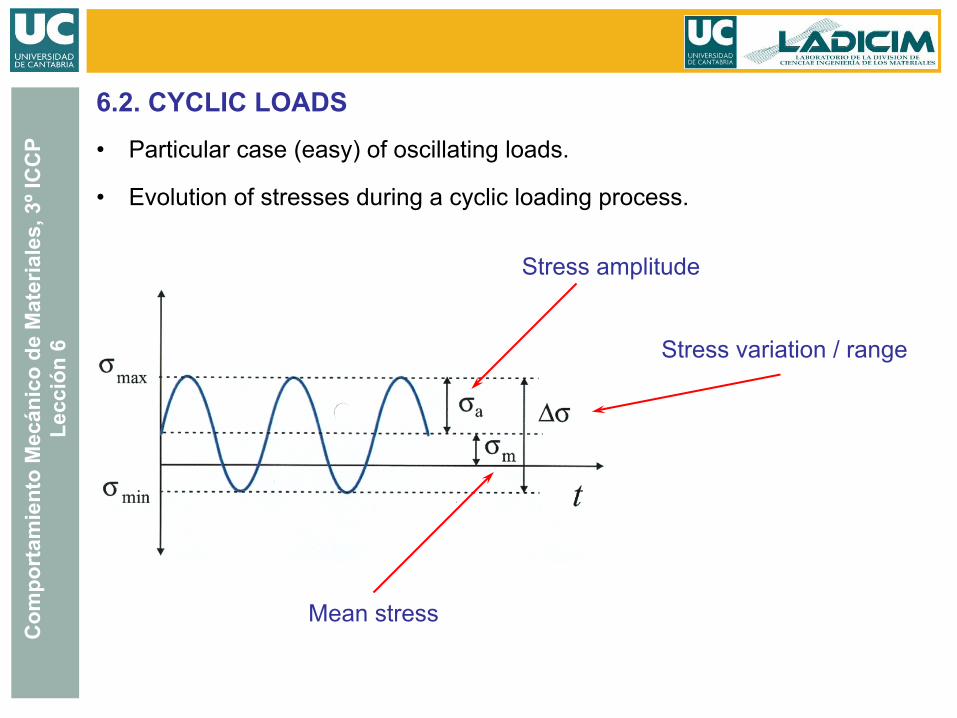
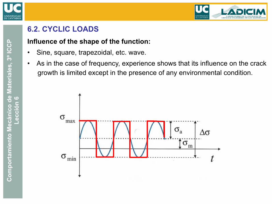
6.2. CYCLIC LOADS
• Particular case (easy) of oscillating loads.
• Evolution of stresses during a cyclic loading process.
Stress variation / range
Stress amplitude
Mean stress
Com
port
amie
nto
Mec
ánic
o de
Mat
eria
les,
3º I
CC
P Le
cció
n 6
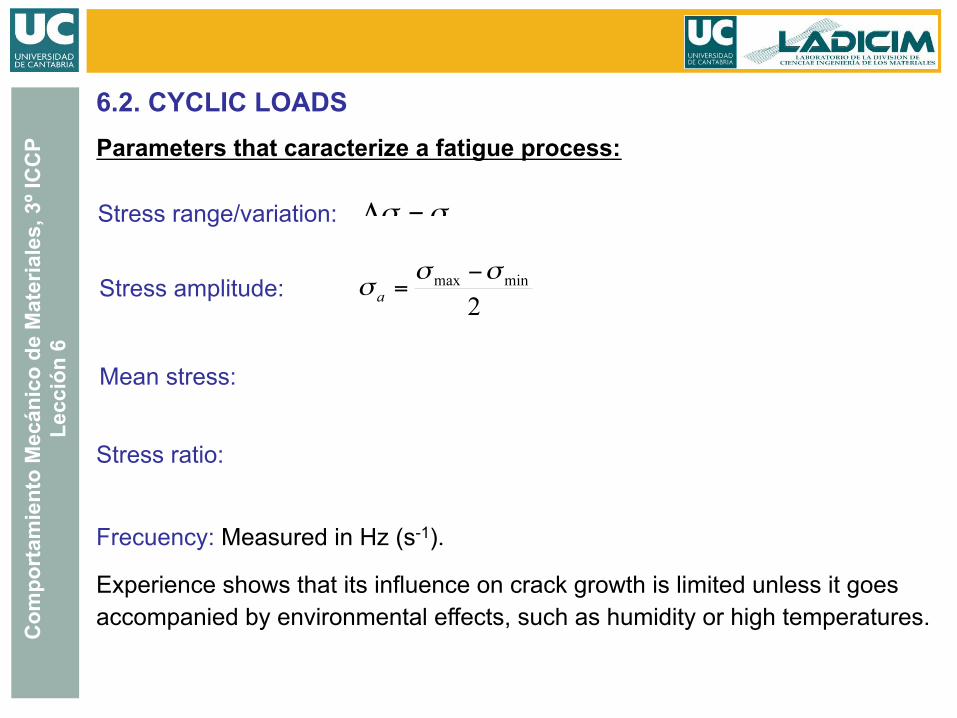
Parameters that caracterize a fatigue process:
Frecuency: Measured in Hz (s-1).
Experience shows that its influence on crack growth is limited unless it goes accompanied by environmental effects, such as humidity or high temperatures.
6.2. CYCLIC LOADS
Stress amplitude:
Stress range/variation:
Mean stress:
Stress ratio:
Com
port
amie
nto
Mec
ánic
o de
Mat
eria
les,
3º I
CC
P Le
cció
n 6
6.2. CYCLIC LOADS Influence of the shape of the function: • Sine, square, trapezoidal, etc. wave. • As in the case of frequency, experience shows that its influence on the crack
growth is limited except in the presence of any environmental condition.
Com
port
amie
nto
Mec
ánic
o de
Mat
eria
les,
3º I
CC
P Le
cció
n 6
6.2. CYCLIC LOADS Suggested exercises:
1) Obtain the mean stress, stress amplitude and stress range assuming: σmin = -100 MPa y σmax=250 MPa.
Com
port
amie
nto
Mec
ánic
o de
Mat
eria
les,
3º I
CC
P Le
cció
n 6
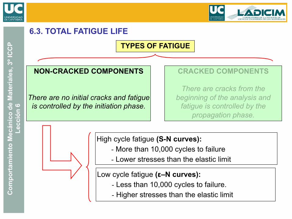
6.3. TOTAL FATIGUE LIFE
TYPES OF FATIGUE
NON-CRACKED COMPONENTS
There are no initial cracks and fatigue is controlled by the initiation phase.
High cycle fatigue (S-N curves): - More than 10,000 cycles to failure - Lower stresses than the elastic limit
CRACKED COMPONENTS
There are cracks from the beginning of the analysis and
fatigue is controlled by the propagation phase.
Low cycle fatigue (ε–N curves): - Less than 10,000 cycles to failure. - Higher stresses than the elastic limit
Com
port
amie
nto
Mec
ánic
o de
Mat
eria
les,
3º I
CC
P Le
cció
n 6
6.3. TOTAL FATIGUE LIFE
• It was the first approach of fatigue analysis: presented by Wöhler (1860). • Sine, square, trapezoidal, etc. wave. • It includes the processes of crack initiation, propagation and final
fracture of the component. • There are two analysis methods of fatigue based on total life
considerations: • HIGH CYCLE FATIGUE (HCF): S-N curve (Wöhler curve) • LOW CYCLE FATIGUE (LCF): ε-N curve
Com
port
amie
nto
Mec
ánic
o de
Mat
eria
les,
3º I
CC
P Le
cció
n 6
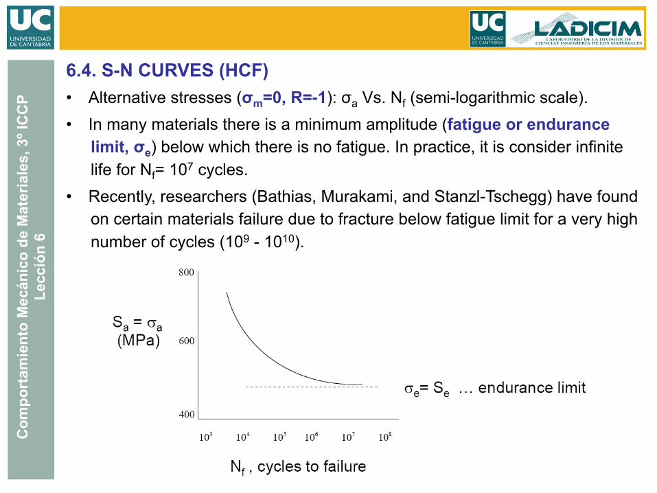
6.4. S-N CURVES (HCF) • Alternative stresses (σm=0, R=-1): σa Vs. Nf (semi-logarithmic scale). • In many materials there is a minimum amplitude (fatigue or endurance
limit, σe) below which there is no fatigue. In practice, it is consider infinite life for Nf= 107 cycles.
• Recently, researchers (Bathias, Murakami, and Stanzl-Tschegg) have found on certain materials failure due to fracture below fatigue limit for a very high number of cycles (109 - 1010).
Com
port
amie
nto
Mec
ánic
o de
Mat
eria
les,
3º I
CC
P Le
cció
n 6
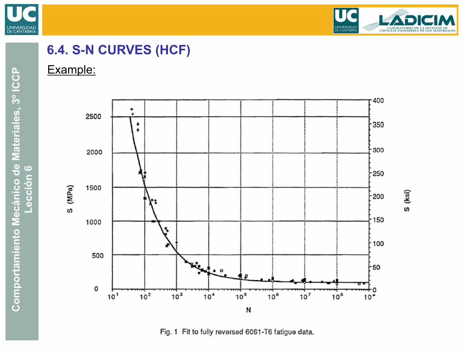
6.4. S-N CURVES (HCF) Example:
Com
port
amie
nto
Mec
ánic
o de
Mat
eria
les,
3º I
CC
P Le
cció
n 6
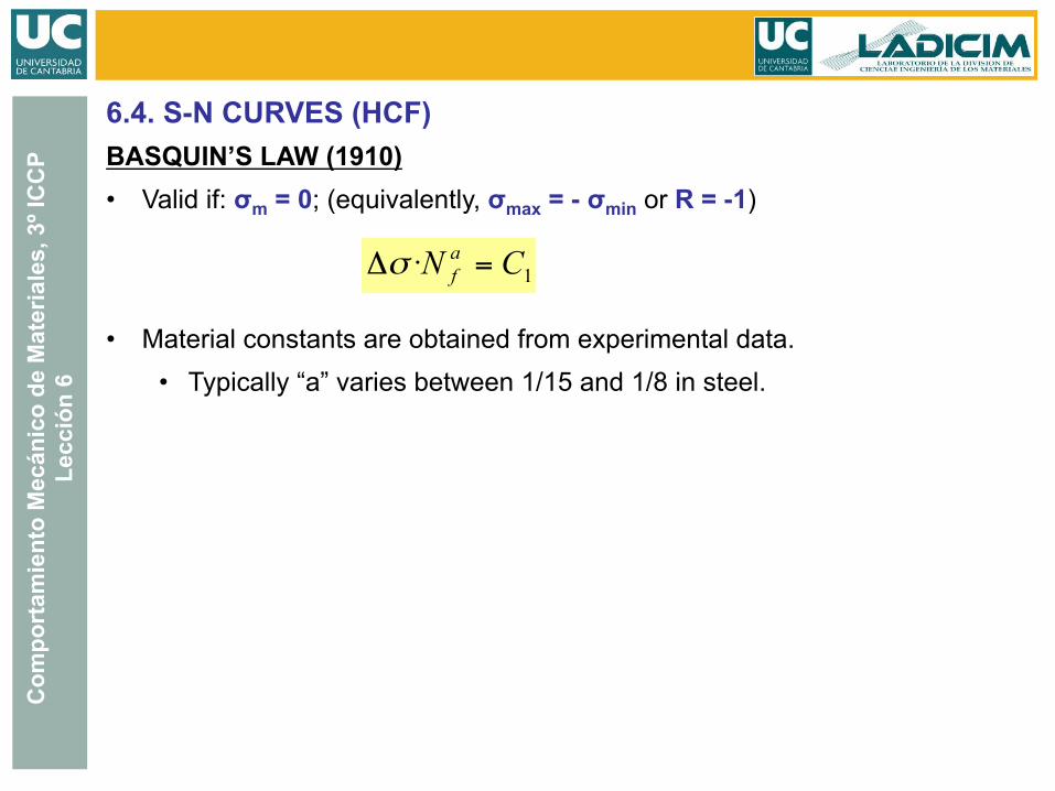
6.4. S-N CURVES (HCF) BASQUIN’S LAW (1910) • Valid if: σm = 0; (equivalently, σmax = - σmin or R = -1)
• Material constants are obtained from experimental data. • Typically “a” varies between 1/15 and 1/8 in steel.
Com
port
amie
nto
Mec
ánic
o de
Mat
eria
les,
3º I
CC
P Le
cció
n 6
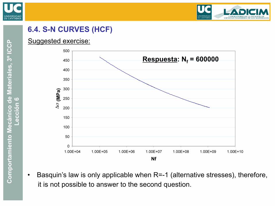
Suggested exercise:
1) Apply Basquin’s law to estimate the number of cycles resisted by a structural component subjected to the following conditions:
σmin=-200 MPa; σmax=200 MPa; a=0.090; C1=1320
Is it possible to answer the same question if σmin=-200 MPa and σmax=200 MPa? Justify the answer
6.4. S-N CURVES (HCF)
Com
port
amie
nto
Mec
ánic
o de
Mat
eria
les,
3º I
CC
P Le
cció
n 6
Suggested exercise: 6.4. S-N CURVES (HCF)
Respuesta: Nf = 600000
• Basquin’s law is only applicable when R=-1 (alternative stresses), therefore, it is not possible to answer to the second question.
Com
port
amie
nto
Mec
ánic
o de
Mat
eria
les,
3º I
CC
P Le
cció
n 6
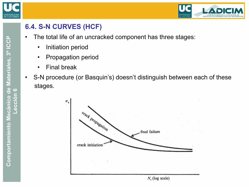
6.4. S-N CURVES (HCF) • The total life of an uncracked component has three stages:
• Initiation period • Propagation period • Final break
• S-N procedure (or Basquin’s) doesn’t distinguish between each of these stages.
Com
port
amie
nto
Mec
ánic
o de
Mat
eria
les,
3º I
CC
P Le
cció
n 6
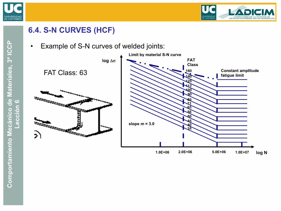
6.4. S-N CURVES (HCF)
• Example of S-N curves of welded joints:
FAT Class: 63
Com
port
amie
nto
Mec
ánic
o de
Mat
eria
les,
3º I
CC
P Le
cció
n 6
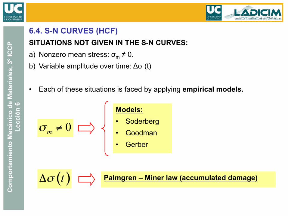
6.4. S-N CURVES (HCF) SITUATIONS NOT GIVEN IN THE S-N CURVES: a) Nonzero mean stress: σm ≠ 0. b) Variable amplitude over time: Δσ (t)
• Each of these situations is faced by applying empirical models.
Models: • Soderberg • Goodman • Gerber
Palmgren – Miner law (accumulated damage)
Com
port
amie
nto
Mec
ánic
o de
Mat
eria
les,
3º I
CC
P Le
cció
n 6
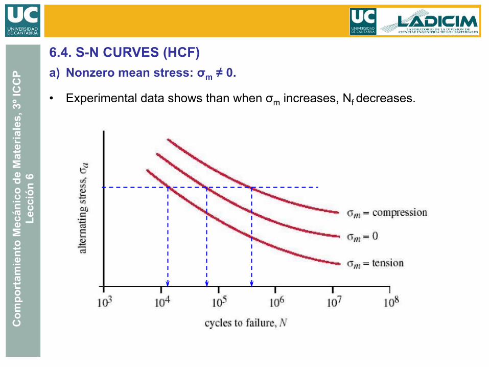
6.4. S-N CURVES (HCF) a) Nonzero mean stress: σm ≠ 0.
• Experimental data shows than when σm increases, Nf decreases.
Com
port
amie
nto
Mec
ánic
o de
Mat
eria
les,
3º I
CC
P Le
cció
n 6
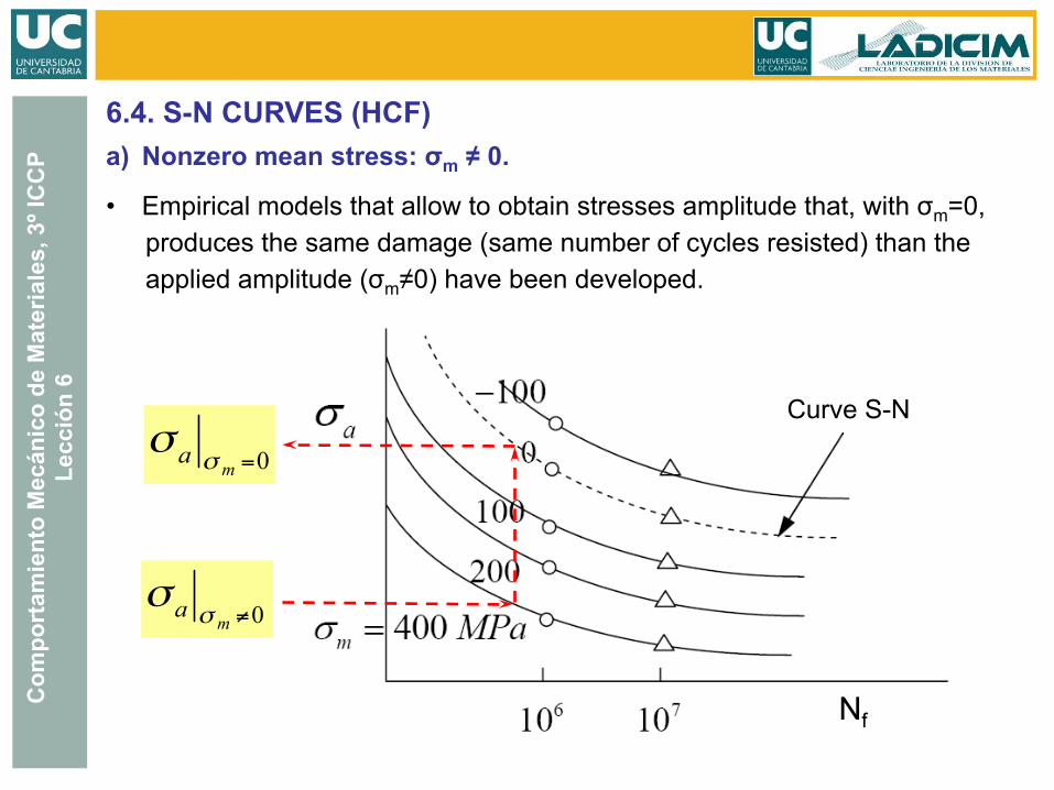
6.4. S-N CURVES (HCF)
• Empirical models that allow to obtain stresses amplitude that, with σm=0, produces the same damage (same number of cycles resisted) than the applied amplitude (σm≠0) have been developed.
a) Nonzero mean stress: σm ≠ 0.
Curve S-N
Com
port
amie
nto
Mec
ánic
o de
Mat
eria
les,
3º I
CC
P Le
cció
n 6
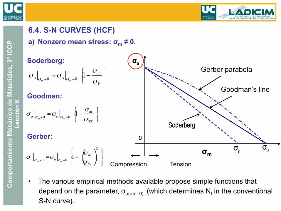
Soderberg:
6.4. S-N CURVES (HCF) a) Nonzero mean stress: σm ≠ 0.
Goodman:
Gerber:
• The various empirical methods available propose simple functions that depend on the parameter, σa(σm=0). (which determines Nf in the conventional S-N curve).
Gerber parabola
Goodman’s line
Tension Compression
Com
port
amie
nto
Mec
ánic
o de
Mat
eria
les,
3º I
CC
P Le
cció
n 6
6.4. S-N CURVES (HCF) a) Nonzero mean stress: σm ≠ 0.
Com
port
amie
nto
Mec
ánic
o de
Mat
eria
les,
3º I
CC
P Le
cció
n 6
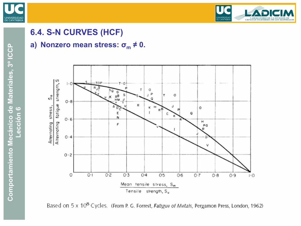
6.4. S-N CURVES (HCF)
GENERAL COMMENTS: • Most of the experimental data are between Gerber and Goodman curves. • The expression proposed by Goodman works well with brittle materials,
being really conservative for ductile materials and, finally, Gerber expression is adequate for ductile materials
• Soderberg’s line is, usually, too conservative (which is not necessarily bad, given the great uncertainties in any fatigue situation).
a) Nonzero stress: σm ≠ 0.
Com
port
amie
nto
Mec
ánic
o de
Mat
eria
les,
3º I
CC
P Le
cció
n 6
6.4. S-N CURVES (HCF) a) Nonzero mean stress: σm ≠ 0.
Com
port
amie
nto
Mec
ánic
o de
Mat
eria
les,
3º I
CC
P Le
cció
n 6
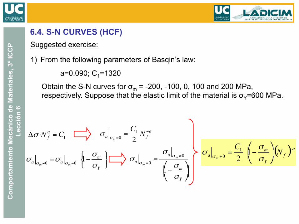
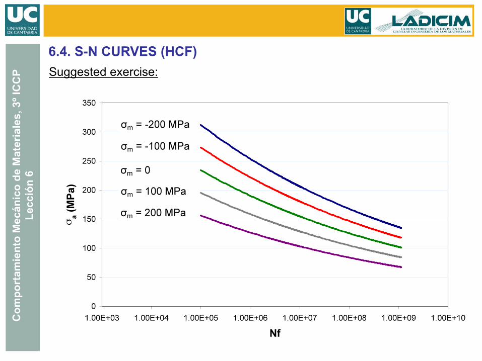
6.4. S-N CURVES (HCF) Suggested exercise:
1) From the following parameters of Basqin’s law:
a=0.090; C1=1320
Obtain the S-N curves for σm = -200, -100, 0, 100 and 200 MPa, respectively. Suppose that the elastic limit of the material is σY=600 MPa.
Com
port
amie
nto
Mec
ánic
o de
Mat
eria
les,
3º I
CC
P Le
cció
n 6
6.4. S-N CURVES (HCF) Suggested exercise:
Com
port
amie
nto
Mec
ánic
o de
Mat
eria
les,
3º I
CC
P Le
cció
n 6
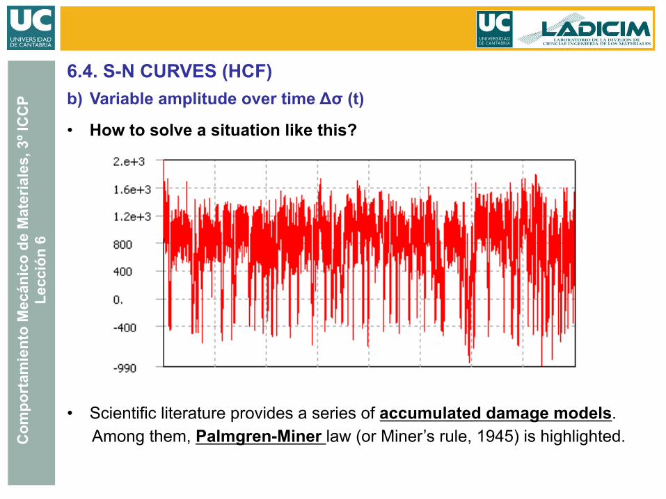
6.4. S-N CURVES (HCF) b) Variable amplitude over time Δσ (t)
• How to solve a situation like this?
• Scientific literature provides a series of accumulated damage models. Among them, Palmgren-Miner law (or Miner’s rule, 1945) is highlighted.
Com
port
amie
nto
Mec
ánic
o de
Mat
eria
les,
3º I
CC
P Le
cció
n 6
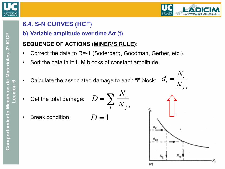
6.4. S-N CURVES (HCF) b) Variable amplitude over time Δσ (t)
SEQUENCE OF ACTIONS (MINER’S RULE): • Correct the data to R=-1 (Soderberg, Goodman, Gerber, etc.). • Sort the data in i=1..M blocks of constant amplitude.
• Calculate the associated damage to each “i” block:
• Get the total damage:
• Break condition:
Com
port
amie
nto
Mec
ánic
o de
Mat
eria
les,
3º I
CC
P Le
cció
n 6
6.4. S-N CURVES (HCF) Suggested exercise:
1) An aluminum alloy, usually used in aeronautical components, presents a behavior in fatigue, analyzed with Basquin’s law, with the parameters a=0.090; C1=1100. A structural component, made with that alloy is still in service after 3.5·108 cycles in the following condition: σa=75 MPa, R=-1.
Determine the maximum admissible stress amplitude to ensure, at least, 10.000 cycles of life remaining (assuming R=-1).
Com
port
amie
nto
Mec
ánic
o de
Mat
eria
les,
3º I
CC
P Le
cció
n 6
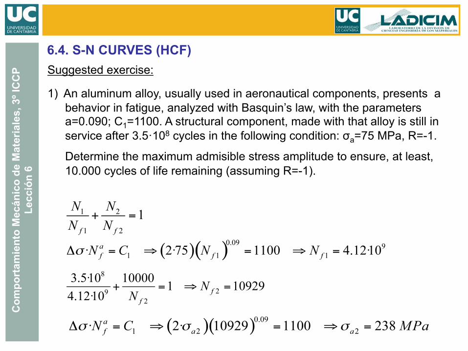
6.4. S-N CURVES (HCF) Suggested exercise:
1) An aluminum alloy, usually used in aeronautical components, presents a behavior in fatigue, analyzed with Basquin’s law, with the parameters a=0.090; C1=1100. A structural component, made with that alloy is still in service after 3.5·108 cycles in the following condition: σa=75 MPa, R=-1.
Determine the maximum admisible stress amplitude to ensure, at least, 10.000 cycles of life remaining (assuming R=-1).
Com
port
amie
nto
Mec
ánic
o de
Mat
eria
les,
3º I
CC
P Le
cció
n 6
6.4. S-N CURVES (HCF) b) Variable amplitude over time Δσ (t)
GENERAL COMMENTS: • It is an approximate but useful model. However, it has some significant
limitations: • It ignores the intrinsically random nature of fatigue processes. • Miner’s rule considers that each block operates independently of one
another. Therefore, it does not consider that the order in which the sequences of blocks with constant amplitude is applied can significantly affect the final result. In some cases, blocks with a low amplitude followed by others with a higher amplitude cause a greater damage than what the model predicts.
• It doesn’t allow to take into account the effects of overloading (which can slow down the movement of a crack).
Com
port
amie
nto
Mec
ánic
o de
Mat
eria
les,
3º I
CC
P Le
cció
n 6
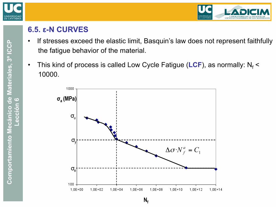
6.5. ε-N CURVES • If stresses exceed the elastic limit, Basquin’s law does not represent faithfully
the fatigue behavior of the material.
• This kind of process is called Low Cycle Fatigue (LCF), as normally: Nf < 10000.
Com
port
amie
nto
Mec
ánic
o de
Mat
eria
les,
3º I
CC
P Le
cció
n 6
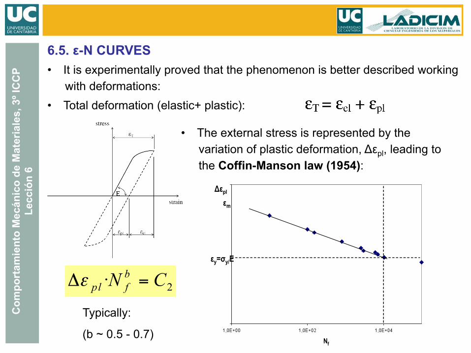
6.5. ε-N CURVES • It is experimentally proved that the phenomenon is better described working
with deformations: • Total deformation (elastic+ plastic):
• The external stress is represented by the variation of plastic deformation, Δεpl, leading to the Coffin-Manson law (1954):
Typically:
(b ~ 0.5 - 0.7)
Com
port
amie
nto
Mec
ánic
o de
Mat
eria
les,
3º I
CC
P Le
cció
n 6
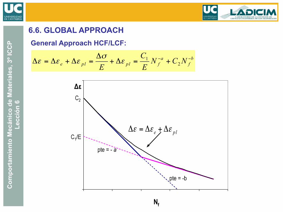
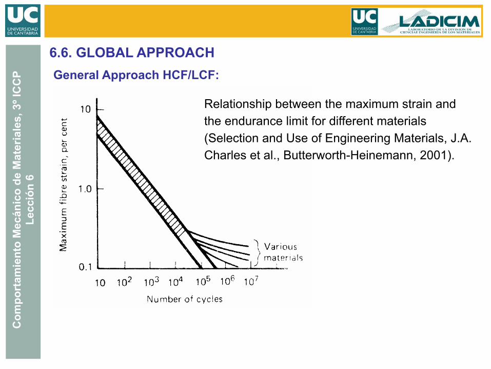
6.6. GLOBAL APPROACH General Approach HCF/LCF:
Com
port
amie
nto
Mec
ánic
o de
Mat
eria
les,
3º I
CC
P Le
cció
n 6
6.6. GLOBAL APPROACH General Approach HCF/LCF:
Relationship between the maximum strain and the endurance limit for different materials (Selection and Use of Engineering Materials, J.A. Charles et al., Butterworth-Heinemann, 2001).
Com
port
amie
nto
Mec
ánic
o de
Mat
eria
les,
3º I
CC
P Le
cció
n 6
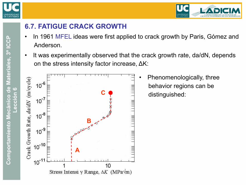
6.7. FATIGUE CRACK GROWTH • In 1961 MFEL ideas were first applied to crack growth by Paris, Gómez and
Anderson. • It was experimentally observed that the crack growth rate, da/dN, depends
on the stress intensity factor increase, ΔK:
• Phenomenologically, three behavior regions can be distinguished:
A
B
C
Com
port
amie
nto
Mec
ánic
o de
Mat
eria
les,
3º I
CC
P Le
cció
n 6
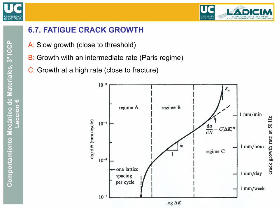
6.7. FATIGUE CRACK GROWTH
A: Slow growth (close to threshold)
B: Growth with an intermediate rate (Paris regime)
C: Growth at a high rate (close to fracture)
Com
port
amie
nto
Mec
ánic
o de
Mat
eria
les,
3º I
CC
P Le
cció
n 6
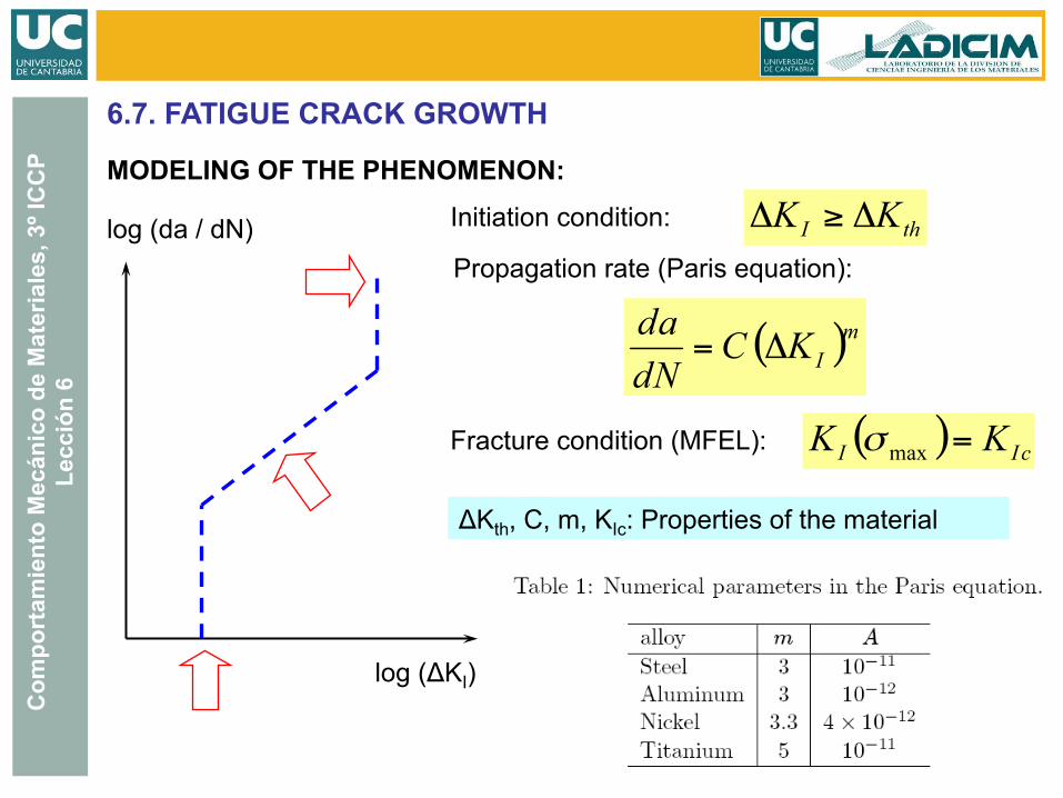
6.7. FATIGUE CRACK GROWTH
MODELING OF THE PHENOMENON:
log (da / dN) Initiation condition:
Propagation rate (Paris equation):
Fracture condition (MFEL):
ΔKth, C, m, KIc: Properties of the material
log (ΔKI)
Com
port
amie
nto
Mec
ánic
o de
Mat
eria
les,
3º I
CC
P Le
cció
n 6
6.7. FATIGUE CRACK GROWTH REGIME A: • Simplified, the FIT range, ΔK, must exceed a threshold ΔKth, that depends
on the material, so that the movement of the crack occurs. • In practice, what happens is that, when ΔK < ΔKth, the crack propagates at
undetectable rates. • Practical definition: When the growth rate of the crack falls below 10–8
mm/cycle, it is considered that the crack has stopped; in this situation, ΔK is called ΔKth.
• This limit represents a mean propagation rate lower than the interatomic space per cycle. How is this possible?
• It is considered that there is a great number of cycles in which there is no movement at all, that is, the crack grows an interatomic space in one cycle and then it stabilizes for several cycles.
Com
port
amie
nto
Mec
ánic
o de
Mat
eria
les,
3º I
CC
P Le
cció
n 6
6.7. FATIGUE CRACK GROWTH
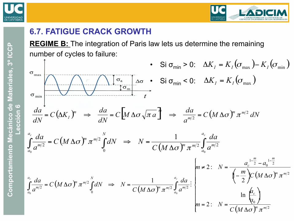
• Si σmin > 0:
• Si σmin < 0:
REGIME B: The integration of Paris law lets us determine the remaining number of cycles to failure:
Com
port
amie
nto
Mec
ánic
o de
Mat
eria
les,
3º I
CC
P Le
cció
n 6
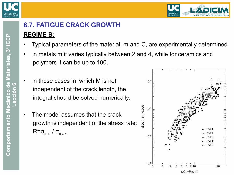
6.7. FATIGUE CRACK GROWTH REGIME B: • Typical parameters of the material, m and C, are experimentally determined
• In metals m it varies typically between 2 and 4, while for ceramics and polymers it can be up to 100.
• In those cases in which M is not independent of the crack length, the integral should be solved numerically.
• The model assumes that the crack growth is independent of the stress rate: R=σmin / σmax.
Com
port
amie
nto
Mec
ánic
o de
Mat
eria
les,
3º I
CC
P Le
cció
n 6
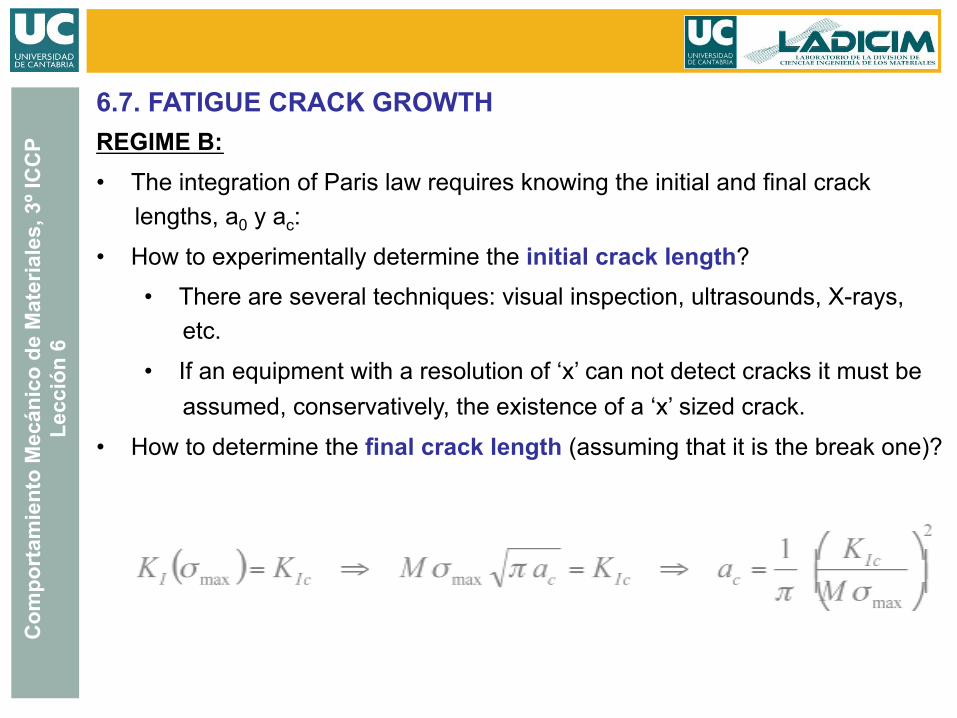
6.7. FATIGUE CRACK GROWTH REGIME B: • The integration of Paris law requires knowing the initial and final crack
lengths, a0 y ac:
• How to experimentally determine the initial crack length?
• There are several techniques: visual inspection, ultrasounds, X-rays, etc.
• If an equipment with a resolution of ‘x’ can not detect cracks it must be assumed, conservatively, the existence of a ‘x’ sized crack.
• How to determine the final crack length (assuming that it is the break one)?
Com
port
amie
nto
Mec
ánic
o de
Mat
eria
les,
3º I
CC
P Le
cció
n 6
From the previous analysis raises a really important idea: Even when there are detected cracks on a component or structure it is not necessary to stop using and remove it!
For this statement to make sense we must evaluate the remaining life. The component can continue working as long as it is periodically inspected
Regime B
6.7. FATIGUE CRACK GROWTH
Com
port
amie
nto
Mec
ánic
o de
Mat
eria
les,
3º I
CC
P Le
cció
n 6
Failure of an structure or a component after a fatigue process can occur by two different mechanisms:
– For high values of ΔK the propagation rate grows really fast until it gets to the final Fracture when the fracture toughness of the material is reached.
Ex: Many steels at low temperature.
– Plastic collapse of the remaining section.
Ex: Room temperature in ductile materials.
Regime C
6.7. FATIGUE CRACK GROWTH
Com
port
amie
nto
Mec
ánic
o de
Mat
eria
les,
3º I
CC
P Le
cció
n 6
Objective: Determination of Paris law.
Methodology: Based on MFEL crack propagation rate is determined depending on ΔK.
1. Election of the typical specimen in MF (CT,SENB,...)
2. Load application system (Constant amplitude)
3. Crack propagation tracking method depending on N.
4. Obtaining the mean propagation rate in zone II.
5. Threshold determination ΔKth
6.Logarithmical representation of da/dN-log ΔK and adjustment with Paris parameters.
Normative: ASTM E-647
6.8. DETERMINATION OF PARIS LAW
Com
port
amie
nto
Mec
ánic
o de
Mat
eria
les,
3º I
CC
P Le
cció
n 6
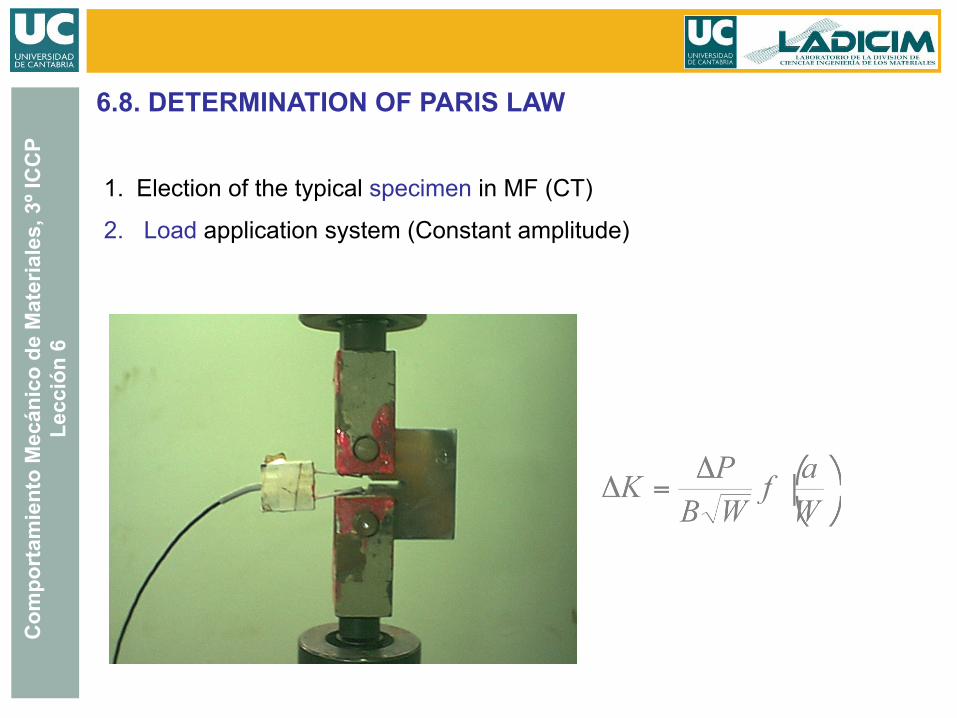
1. Election of the typical specimen in MF (CT)
2. Load application system (Constant amplitude)
6.8. DETERMINATION OF PARIS LAW
Com
port
amie
nto
Mec
ánic
o de
Mat
eria
les,
3º I
CC
P Le
cció
n 6
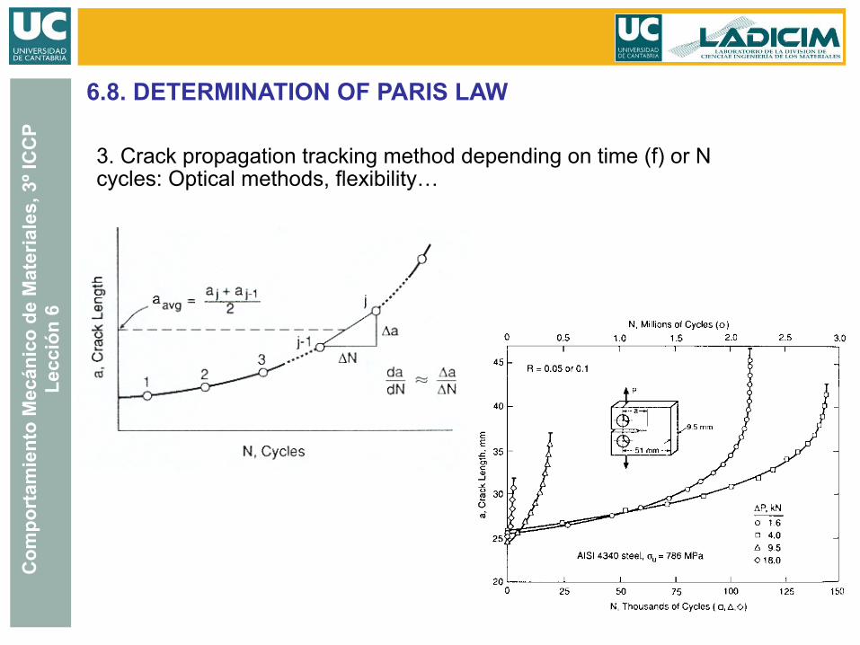
3. Crack propagation tracking method depending on time (f) or N cycles: Optical methods, flexibility…
6.8. DETERMINATION OF PARIS LAW
Com
port
amie
nto
Mec
ánic
o de
Mat
eria
les,
3º I
CC
P Le
cció
n 6
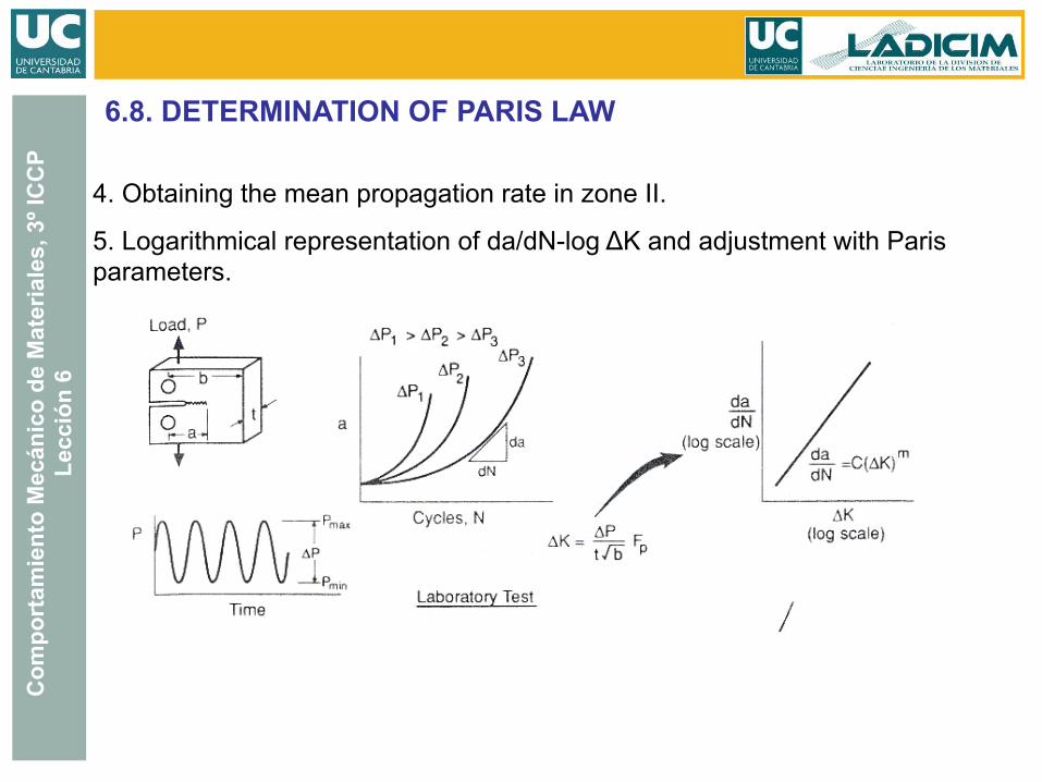
4. Obtaining the mean propagation rate in zone II.
5. Logarithmical representation of da/dN-log ΔK and adjustment with Paris parameters.
5. Threshold determination ΔKth
6.8. DETERMINATION OF PARIS LAW
Com
port
amie
nto
Mec
ánic
o de
Mat
eria
les,
3º I
CC
P Le
cció
n 6
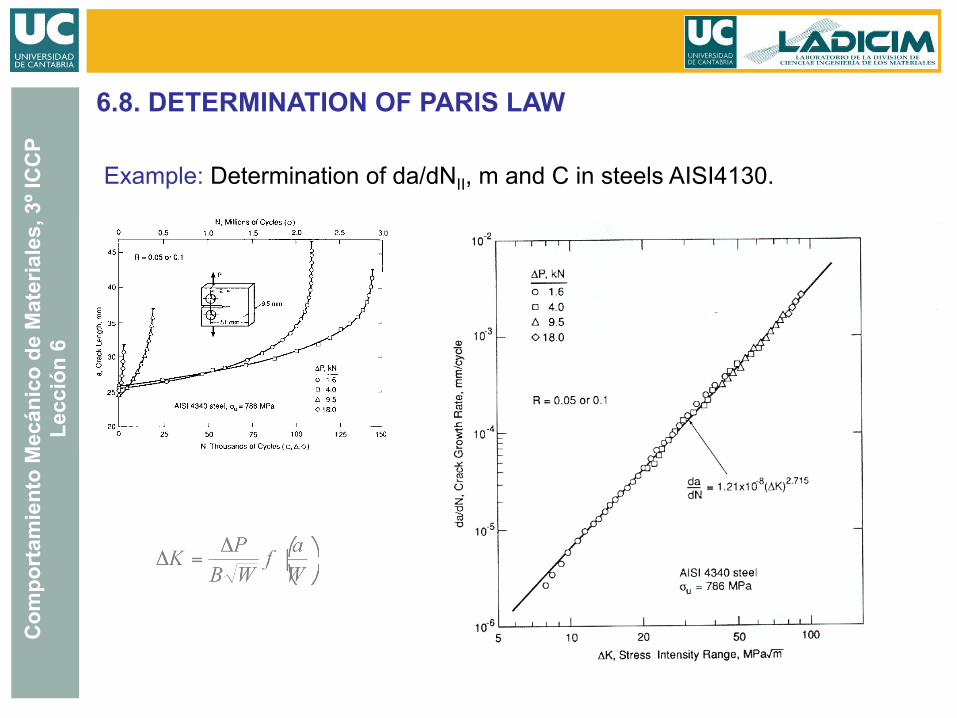
Example: Determination of da/dNII, m and C in steels AISI4130.
6.8. DETERMINATION OF PARIS LAW
Com
port
amie
nto
Mec
ánic
o de
Mat
eria
les,
3º I
CC
P Le
cció
n 6
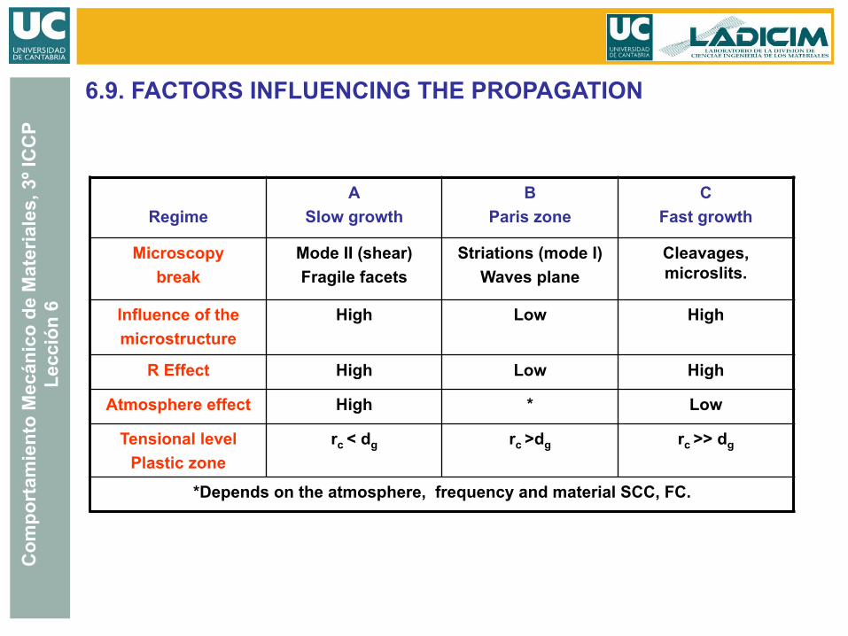
Regime A
Slow growth B
Paris zone C
Fast growth
Microscopy break
Mode II (shear) Fragile facets
Striations (mode I) Waves plane
Cleavages, microslits.
Influence of the microstructure
High Low High
R Effect High Low High
Atmosphere effect High * Low
Tensional level Plastic zone
rc < dg rc >dg rc >> dg
*Depends on the atmosphere, frequency and material SCC, FC.
6.9. FACTORS INFLUENCING THE PROPAGATION
Com
port
amie
nto
Mec
ánic
o de
Mat
eria
les,
3º I
CC
P Le
cció
n 6
6.10. FATIGUE MICROMECHANISM
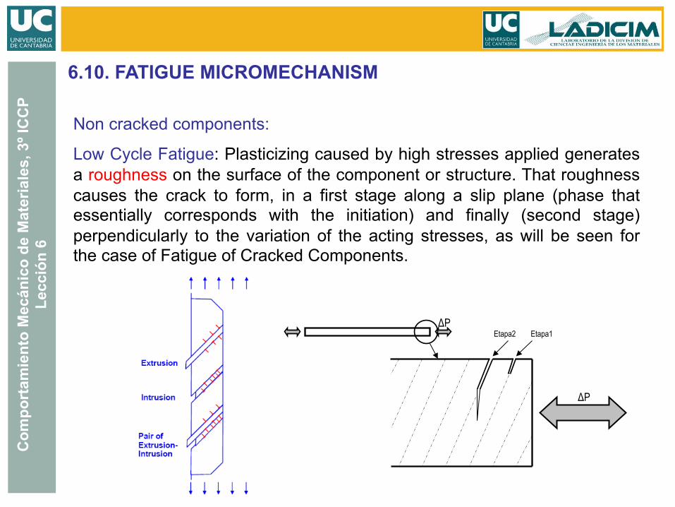
Non cracked components:
Low Cycle Fatigue: Plasticizing caused by high stresses applied generates a roughness on the surface of the component or structure. That roughness causes the crack to form, in a first stage along a slip plane (phase that essentially corresponds with the initiation) and finally (second stage) perpendicularly to the variation of the acting stresses, as will be seen for the case of Fatigue of Cracked Components.
ΔP
ΔP Etapa1 Etapa2
Com
port
amie
nto
Mec
ánic
o de
Mat
eria
les,
3º I
CC
P Le
cció
n 6
Non cracked components
High Cycle Fatigue: even if the applied stress is lower than the elastic limit, there will be a local plasticization wherever there is a notch, a scratch or a change in section that acts as a stress concentrator. This local plasticization will generate the appearance of cracks in a similar way as it occurs in Low Cycle Fatigue, consuming the initiation of most part of fatigue life.
From all that has been said, we can deduce that the existence of stress concentrators greatly limits the fatigue life of High Cycle Fatigue.
6.10. FATIGUE MICROMECHANISM
Com
port
amie
nto
Mec
ánic
o de
Mat
eria
les,
3º I
CC
P Le
cció
n 6
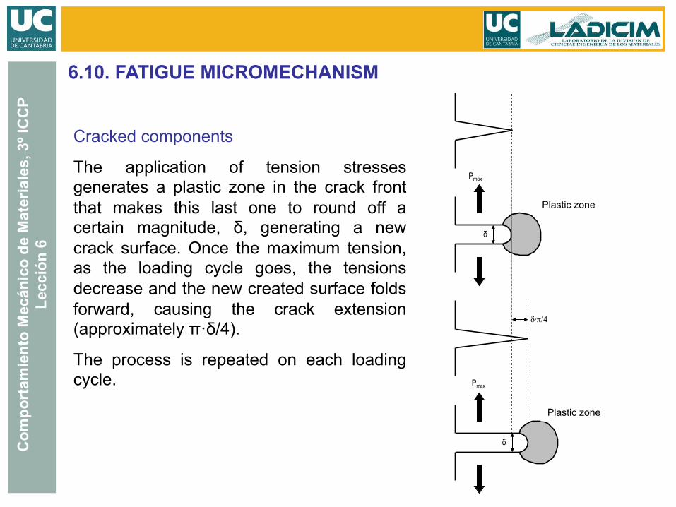
Cracked components
The application of tension stresses generates a plastic zone in the crack front that makes this last one to round off a certain magnitude, δ, generating a new crack surface. Once the maximum tension, as the loading cycle goes, the tensions decrease and the new created surface folds forward, causing the crack extension (approximately π·δ/4).
The process is repeated on each loading cycle.
δ
δ
δ·π/4
Zona Plástica
Zona Plástica
Pmax
Pmax
6.10. FATIGUE MICROMECHANISM
Plastic zone
Plastic zone
Com
port
amie
nto
Mec
ánic
o de
Mat
eria
les,
3º I
CC
P Le
cció
n 6
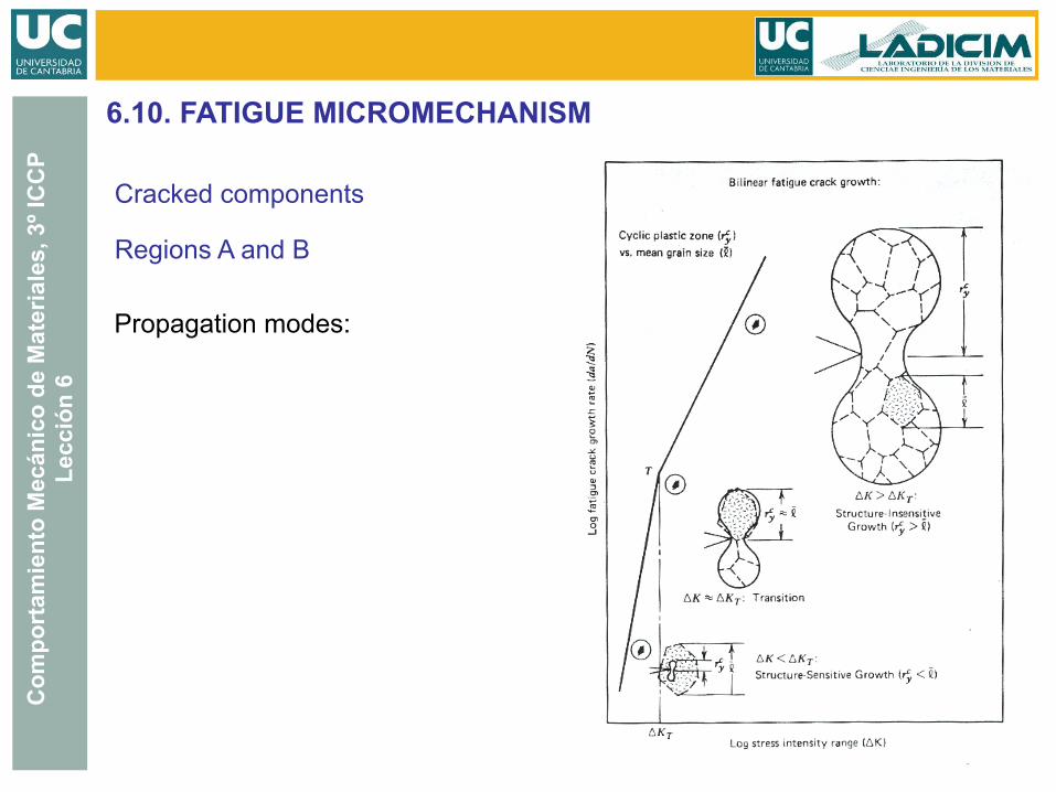
Propagation modes:
Cracked components
Regions A and B
6.10. FATIGUE MICROMECHANISM
Com
port
amie
nto
Mec
ánic
o de
Mat
eria
les,
3º I
CC
P Le
cció
n 6
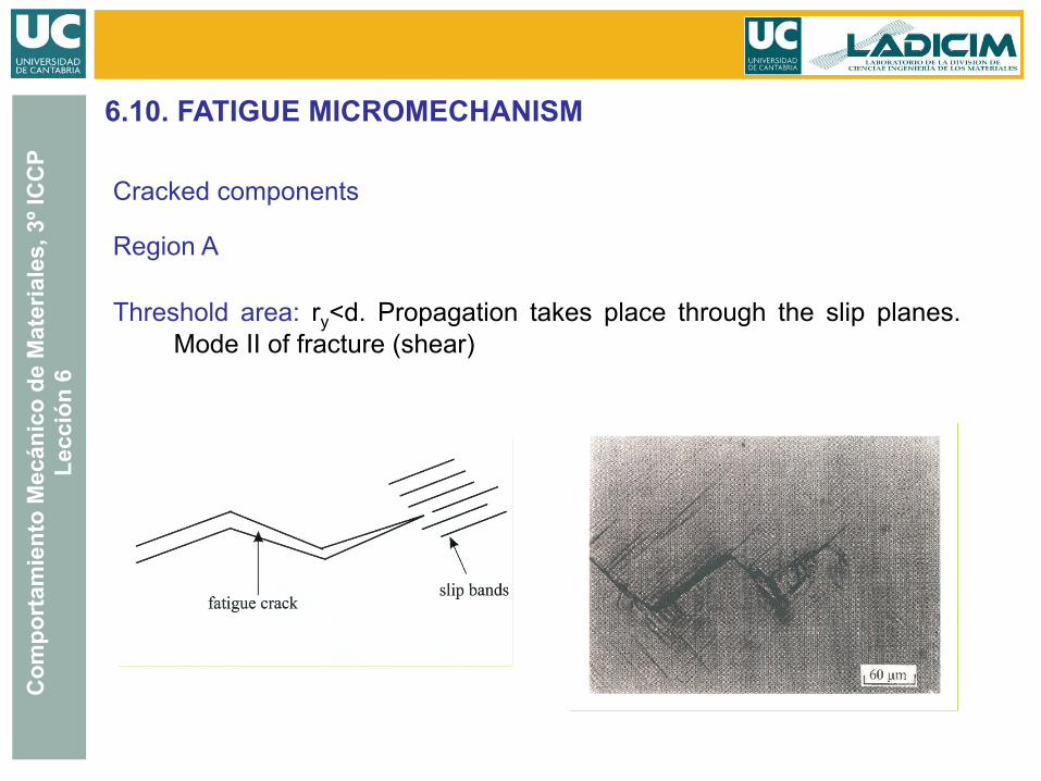
Threshold area: ry<d. Propagation takes place through the slip planes. Mode II of fracture (shear)
Cracked components
Region A
6.10. FATIGUE MICROMECHANISM
Com
port
amie
nto
Mec
ánic
o de
Mat
eria
les,
3º I
CC
P Le
cció
n 6
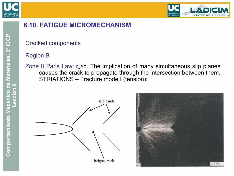
Zone II Paris Law: ry>d. The implication of many simultaneous slip planes causes the crack to propagate through the intersection between them. STRIATIONS – Fracture mode I (tension):
Cracked components
Region B
6.10. FATIGUE MICROMECHANISM
Com
port
amie
nto
Mec
ánic
o de
Mat
eria
les,
3º I
CC
P Le
cció
n 6
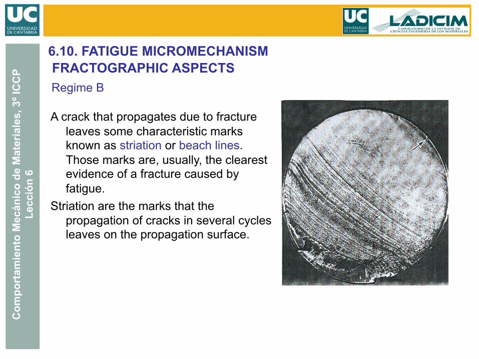
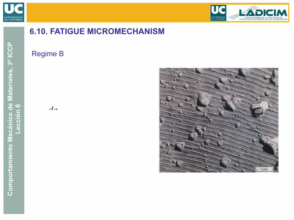
A crack that propagates due to fracture leaves some characteristic marks known as striation or beach lines. Those marks are, usually, the clearest evidence of a fracture caused by fatigue.
Striation are the marks that the propagation of cracks in several cycles leaves on the propagation surface.
FRACTOGRAPHIC ASPECTS Regime B
6.10. FATIGUE MICROMECHANISM
Com
port
amie
nto
Mec
ánic
o de
Mat
eria
les,
3º I
CC
P Le
cció
n 6
Regime B
6.10. FATIGUE MICROMECHANISM
Com
port
amie
nto
Mec
ánic
o de
Mat
eria
les,
3º I
CC
P Le
cció
n 6
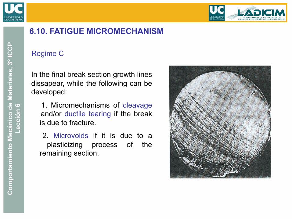
In the final break section growth lines dissapear, while the following can be developed:
1. Micromechanisms of cleavage and/or ductile tearing if the break is due to fracture.
2. Microvoids if it is due to a plasticizing process of the remaining section.
Regime C
6.10. FATIGUE MICROMECHANISM
Com
port
amie
nto
Mec
ánic
o de
Mat
eria
les,
3º I
CC
P Le
cció
n 6
Philosophy: Crack free elements Stages:
– Determination of load spectrum – Estimate the useful life of the material with laboratory tests. – A safety coefficient is applied. – Initiation of crack propagation. At the end of the estimated life, the
component is removed even when it still has left a remarkable life. – Periodic inspections. – Ex: Pressure vessel, jet engines.
SAFE-LIFE
6.11. FATIGUE DESIGN
Com
port
amie
nto
Mec
ánic
o de
Mat
eria
les,
3º I
CC
P Le
cció
n 6
Philosophy: Presence of cracks, tolerable until the reach a critical size.
Periodic inspections: Design of inspection periods to detect the crack before it reaches the critical size.
Stages:
- A component is removed when its estimated life is coming to an end: Detectable crack smaller than critical size.
- Ex: aeronautical industry.
FAIL-SAFE/ Tolerable damage
6.11. FATIGUE DESIGN
Com
port
amie
nto
Mec
ánic
o de
Mat
eria
les,
3º I
CC
P Le
cció
n 6
Approach: Fatigue problems analysis in gas turbines of the type F-100 used in airplanes F-15 and F-16 of USAF
Traditional approach (Safe-life) After a statistical study, 1000 pieces were removed when only one of them had a crack that was <0.75 mm.
REAL CASE
New approach (Fail-Safe) From 1986 to 2005, 3200 engines of the USAF inventory were analyzed. In each engine, 23 components were analyzed. Save foreseen by not justified removals: 1,000,000,000$.
6.11. FATIGUE DESIGN