Lesson 11 - 2

Carrying OutSignificance Tests

Knowledge Objectives

• Identify and explain the four steps involved in formal hypothesis testing.

Construction Objectives

• Using the Inference Toolbox, conduct a z test for a population mean.

• Explain the relationship between a level α two-sided significance test for µ and a level 1 – α confidence interval for µ .

• Conduct a two-sided significance test for µ using a confidence interval.

Vocabulary• Hypothesis – a statement or claim regarding a characteristic of

one or more populations

• Hypothesis Testing – procedure, base on sample evidence and probability, used to test hypotheses

• Null Hypothesis – H0, is a statement to be tested; assumed to be true until evidence indicates otherwise

• Alternative Hypothesis – H1, is a claim to be tested.(what we will test to see if evidence supports the possibility)

• Level of Significance – probability of making a Type I error, α

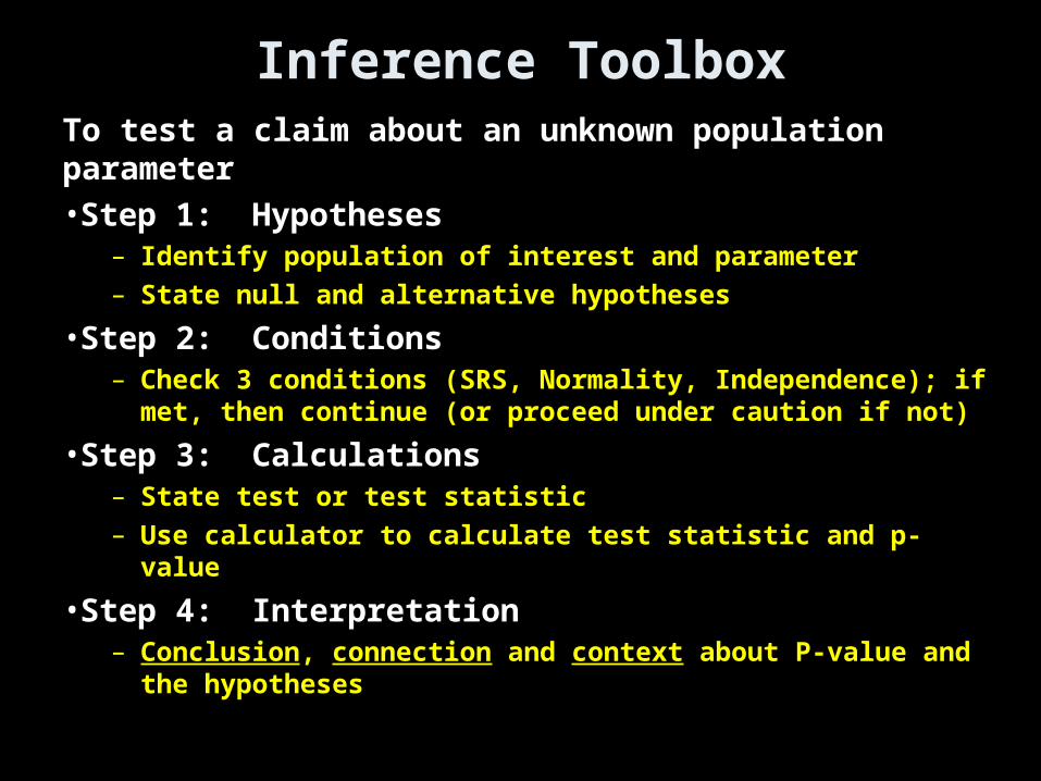
Inference ToolboxTo test a claim about an unknown population parameter•Step 1: Hypotheses

– Identify population of interest and parameter– State null and alternative hypotheses

•Step 2: Conditions– Check 3 conditions (SRS, Normality, Independence); if met,

then continue (or proceed under caution if not)

•Step 3: Calculations– State test or test statistic– Use calculator to calculate test statistic and p-value

•Step 4: Interpretation– Conclusion, connection and context about P-value and the

hypotheses

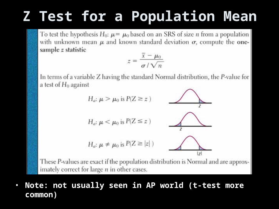
Z Test for a Population Mean

• Note: not usually seen in AP world (t-test more common)

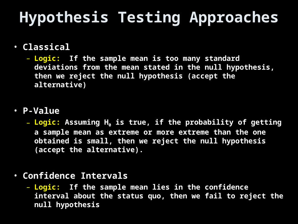
Hypothesis Testing Approaches

• Classical– Logic: If the sample mean is too many standard deviations

from the mean stated in the null hypothesis, then we reject the null hypothesis (accept the alternative)

• P-Value– Logic: Assuming H0 is true, if the probability of getting a

sample mean as extreme or more extreme than the one obtained is small, then we reject the null hypothesis (accept the alternative).

• Confidence Intervals– Logic: If the sample mean lies in the confidence interval about

the status quo, then we fail to reject the null hypothesis

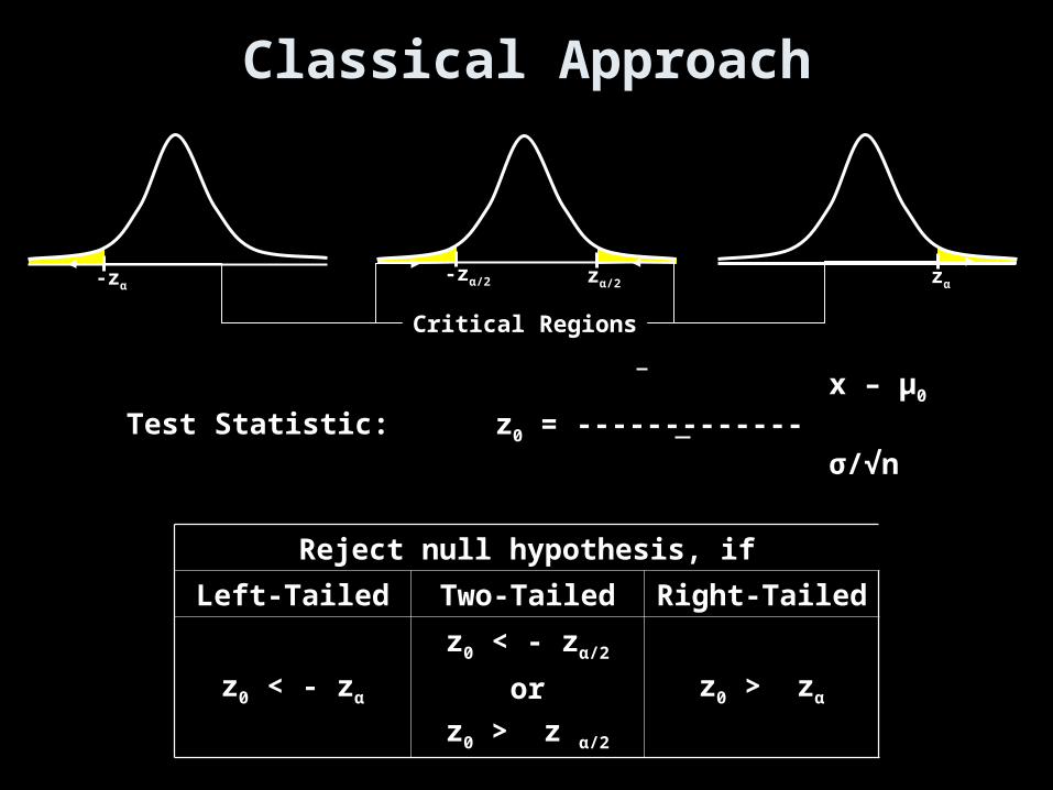
zα-zα/2 zα/2-zα

Critical Regions

x – μ0

Test Statistic: z0 = ------------- σ/√n

Reject null hypothesis, if

Left-Tailed Two-Tailed Right-Tailed

z0 < - zα

z0 < - zα/2

or

z0 > z α/2

z0 > zα

Classical Approach

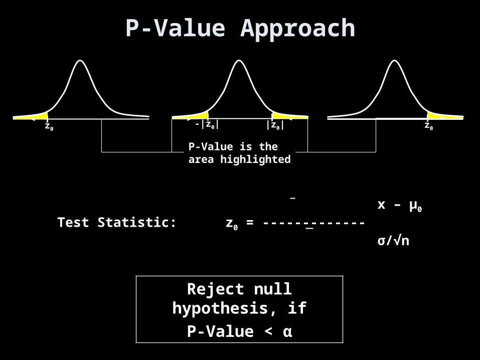
z0-|z0| |z0|z0

P-Value is thearea highlighted

x – μ0

Test Statistic: z0 = ------------- σ/√n

Reject null hypothesis, if

P-Value < α

P-Value Approach

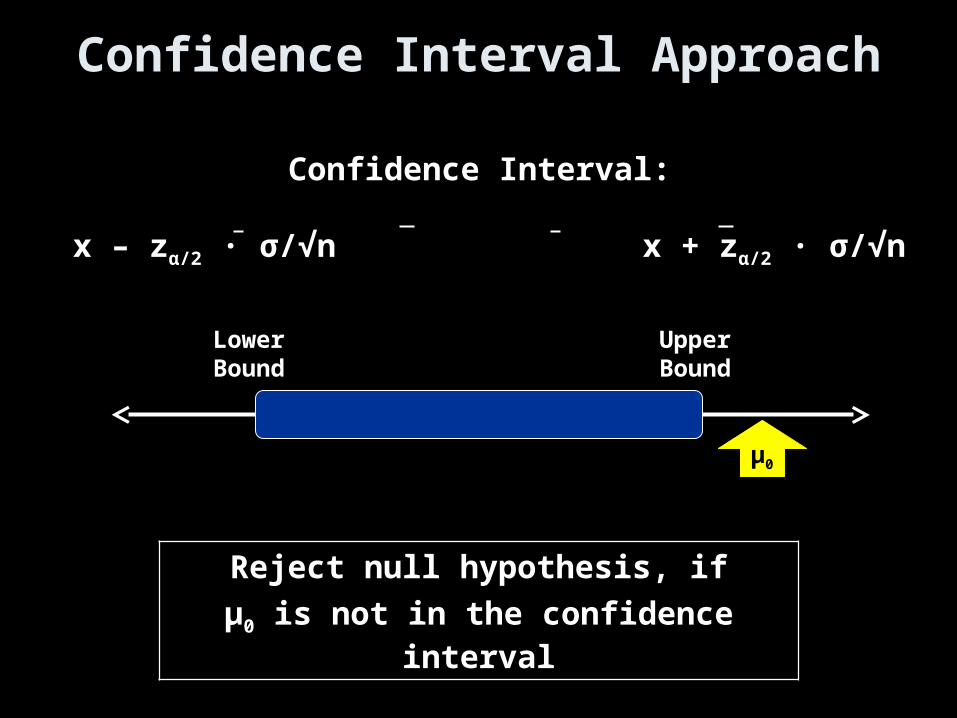
Reject null hypothesis, if

μ0 is not in the confidence interval

Confidence Interval:

x – zα/2 · σ/√n x + zα/2 · σ/√n

Confidence Interval Approach

Lower Bound

Upper Bound

μ0

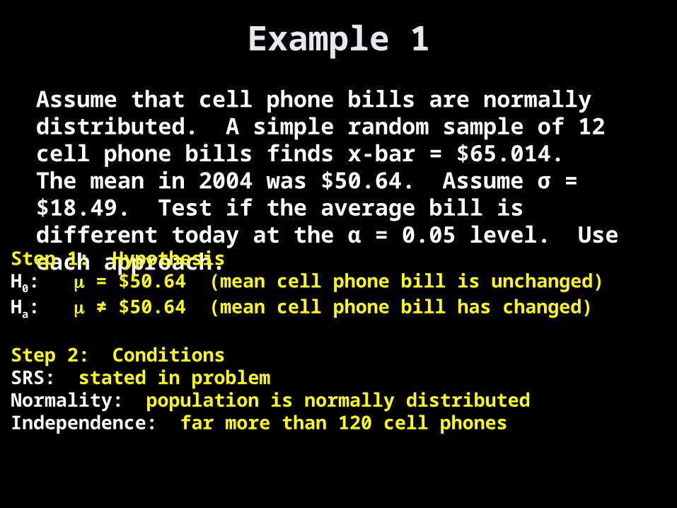
Example 1

Assume that cell phone bills are normally distributed. A simple random sample of 12 cell phone bills finds x-bar = $65.014. The mean in 2004 was $50.64. Assume σ = $18.49. Test if the average bill is different today at the α = 0.05 level. Use each approach.

Step 1: HypothesisH0: = $50.64 (mean cell phone bill is unchanged)Ha: ≠ $50.64 (mean cell phone bill has changed)

Step 2: ConditionsSRS: stated in problemNormality: population is normally distributedIndependence: far more than 120 cell phones

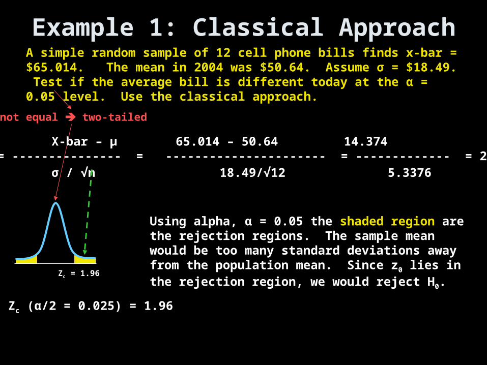
Example 1: Classical ApproachA simple random sample of 12 cell phone bills finds x-bar = $65.014. The mean in 2004 was $50.64. Assume σ = $18.49. Test if the average bill is different today at the α = 0.05 level. Use the classical approach.

not equal two-tailed

Using alpha, α = 0.05 the shaded region are the rejection regions. The sample mean would be too many standard deviations away from the population mean. Since z0 lies in the rejection region, we would reject H0.

Zc = 1.96

Zc (α/2 = 0.025) = 1.96

X-bar – μ 65.014 – 50.64 14.374Z0 = --------------- = ---------------------- = ------------- = 2.69 σ / √n 18.49/√12 5.3376

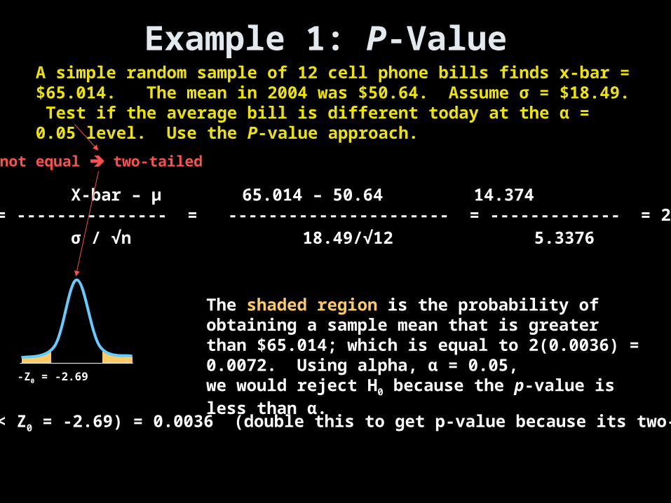
Example 1: P-Value A simple random sample of 12 cell phone bills finds x-bar = $65.014. The mean in 2004 was $50.64. Assume σ = $18.49. Test if the average bill is different today at the α = 0.05 level. Use the P-value approach.

X-bar – μ 65.014 – 50.64 14.374Z0 = --------------- = ---------------------- = ------------- = 2.69 σ / √n 18.49/√12 5.3376

not equal two-tailed

-Z0 = -2.69

The shaded region is the probability of obtaining a sample mean that is greater than $65.014; which is equal to 2(0.0036) = 0.0072. Using alpha, α = 0.05, we would reject H0 because the p-value is less than α.

P( z < Z0 = -2.69) = 0.0036 (double this to get p-value because its two-sided!)

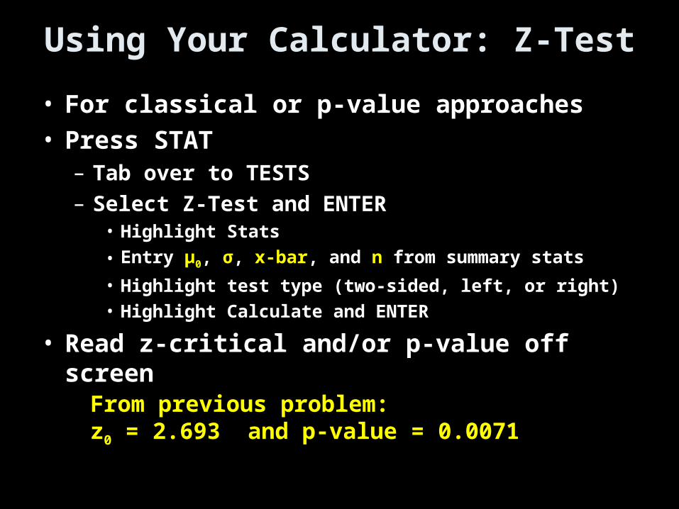
Using Your Calculator: Z-Test

• For classical or p-value approaches• Press STAT– Tab over to TESTS– Select Z-Test and ENTER

• Highlight Stats

• Entry μ0, σ, x-bar, and n from summary stats

• Highlight test type (two-sided, left, or right)• Highlight Calculate and ENTER

• Read z-critical and/or p-value off screen

From previous problem:z0 = 2.693 and p-value = 0.0071

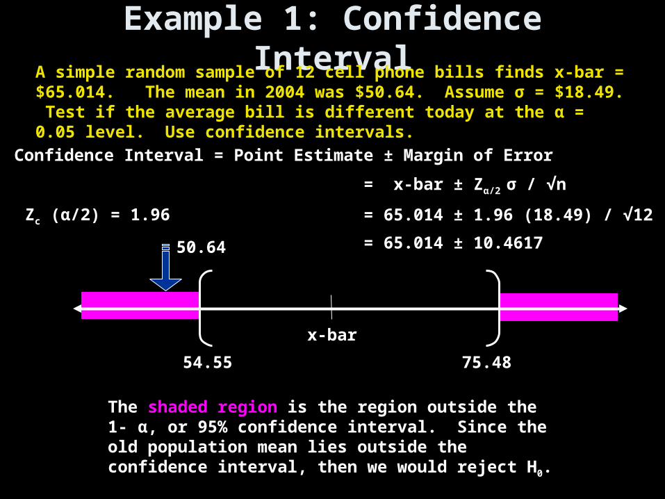
Example 1: Confidence IntervalA simple random sample of 12 cell phone bills finds x-bar = $65.014. The mean in 2004 was $50.64. Assume σ = $18.49. Test if the average bill is different today at the α = 0.05 level. Use confidence intervals.

The shaded region is the region outside the 1- α, or 95% confidence interval. Since the old population mean lies outside the confidence interval, then we would reject H0.

Confidence Interval = Point Estimate ± Margin of Error

= x-bar ± Zα/2 σ / √n

= 65.014 ± 1.96 (18.49) / √12

= 65.014 ± 10.4617

Zc (α/2) = 1.96

50.64

x-bar

54.55 75.48

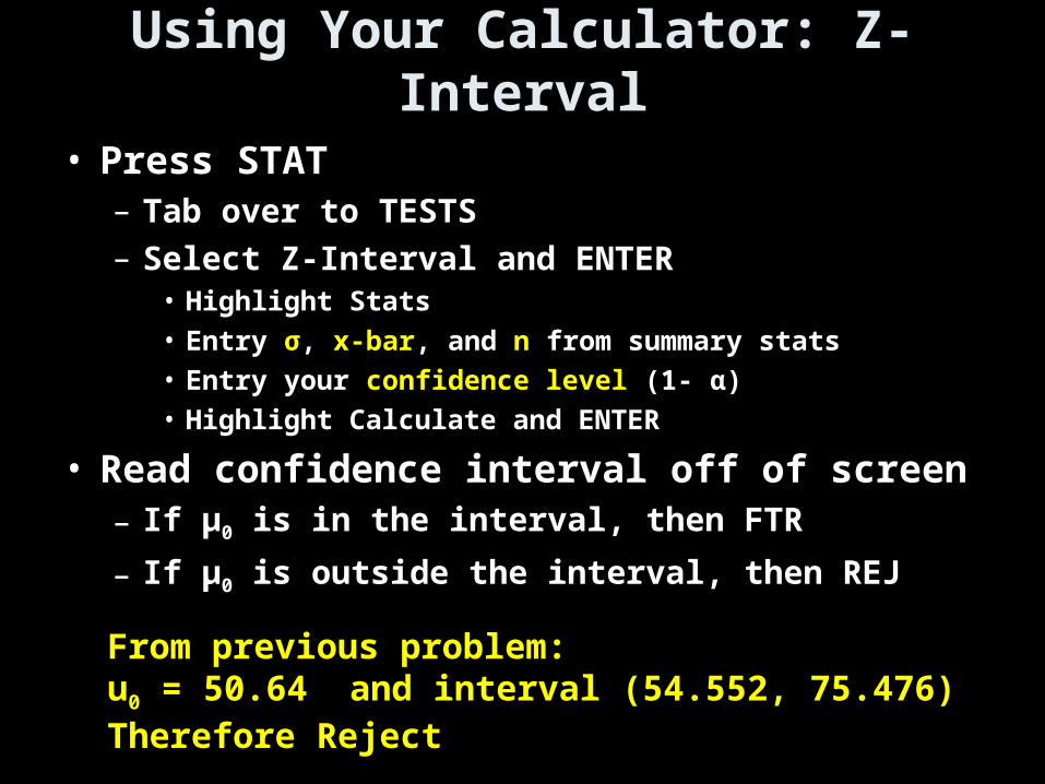
Using Your Calculator: Z-Interval

• Press STAT– Tab over to TESTS– Select Z-Interval and ENTER

• Highlight Stats• Entry σ, x-bar, and n from summary stats• Entry your confidence level (1- α)• Highlight Calculate and ENTER

• Read confidence interval off of screen– If μ0 is in the interval, then FTR

– If μ0 is outside the interval, then REJ

From previous problem:u0 = 50.64 and interval (54.552, 75.476)Therefore Reject

Example 2

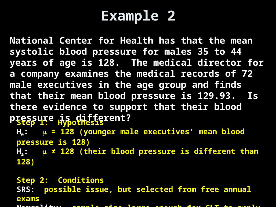
National Center for Health has that the mean systolic blood pressure for males 35 to 44 years of age is 128. The medical director for a company examines the medical records of 72 male executives in the age group and finds that their mean blood pressure is 129.93. Is there evidence to support that their blood pressure is different?

Step 1: HypothesisH0: = 128 (younger male executives’ mean blood pressure is 128)Ha: ≠ 128 (their blood pressure is different than 128)

Step 2: ConditionsSRS: possible issue, but selected from free annual examsNormality: sample size large enough for CLT to applyIndependence: have to assume more than 720 young male executives in the company (large company!!)

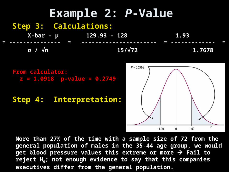
Example 2: P-Value Step 3: Calculations:

Step 4: Interpretation:

X-bar – μ 129.93 – 128 1.93Z0 = --------------- = ---------------------- = ------------- = 1.092 σ / √n 15/√72 1.7678

From calculator: z = 1.0918 p-value = 0.2749

More than 27% of the time with a sample size of 72 from the general population of males in the 35-44 age group, we would get blood pressure values this extreme or more Fail to reject H0; not enough evidence to say that this companies executives differ from the general population.

Example 3Medical director for a large company institutes a health promotion campaign to encourage employees to exercise more and eat a healthier diet. One measure of the effectiveness of such a program is a drop in blood pressure. The director chooses a random sample of 50 employees and compares their blood pressures from physical exams given before the campaign and again a year later. The mean change in systolic blood pressure for these n=50 employees is -6. We take the population standard deviation to be σ=20. The director decides to use an α=0.05 significance level.

Example 3 contHypothesis:

H0:

Ha:

Conditions:

1:

2:

3:

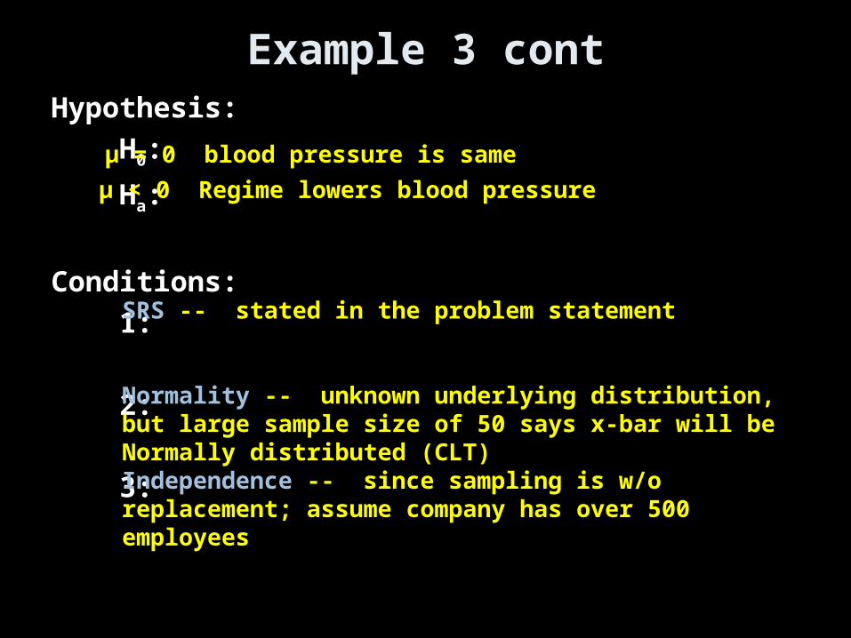
μ = 0 blood pressure is same

μ < 0 Regime lowers blood pressure

SRS -- stated in the problem statement

Normality -- unknown underlying distribution, but large sample size of 50 says x-bar will be Normally distributed (CLT)

Independence -- since sampling is w/o replacement; assume company has over 500 employees

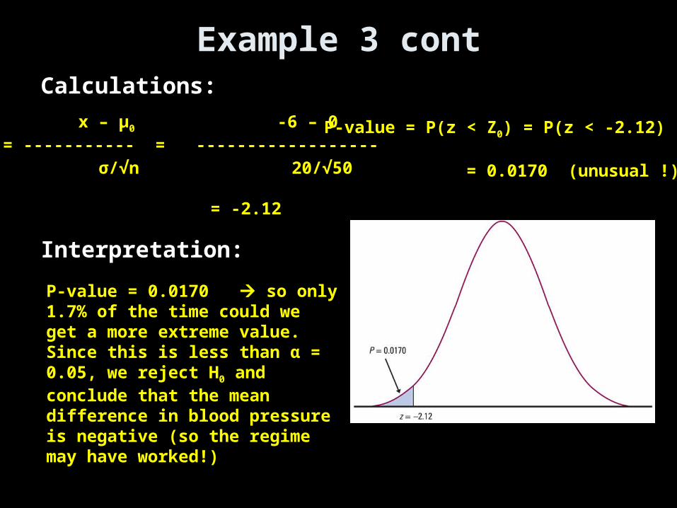
Example 3 contCalculations:

Interpretation:

x – μ0 -6 – 0Z0 = ----------- = ------------------ σ/√n 20/√50

= -2.12

P-value = P(z < Z0) = P(z < -2.12) = 0.0170 (unusual !)

P-value = 0.0170 so only 1.7% of the time could we get a more extreme value. Since this is less than α = 0.05, we reject H0 and conclude that the mean difference in blood pressure is negative (so the regime may have worked!)

Example 4The Deely lab analyzes specimens of a drug to determine the concentration of the active ingredient. The results are not precise and repeated measurements follow a Normal distribution quite closely. The analysis procedure has no bias, so the mean of the population of all measurements is the true concentration of the specimen. The standard deviation of this distribution was found to be σ=0.0068 grams per liter.

A client sends a specimen for which the concentration of active ingredients is supposed to be 0.86%. Deely’s three analyses give concentrations of 0.8403, 0.8363, and 0.8447. Is their significant evidence at the 1% level that the concentration is not 0.86%? Use a confidence interval approach as well as z-test.

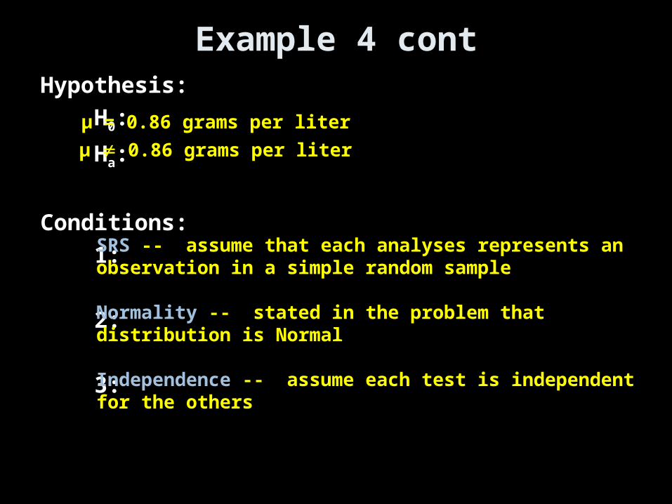
Example 4 contHypothesis:

H0:

Ha:

Conditions:

1:

2:

3:

μ = 0.86 grams per liter

μ 0.86 grams per liter

SRS -- assume that each analyses represents an observation in a simple random sample

Normality -- stated in the problem that distribution is Normal

Independence -- assume each test is independent for the others

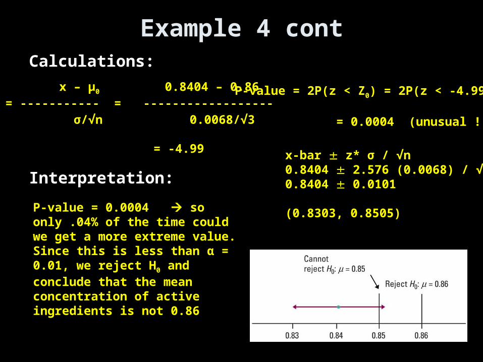
Example 4 contCalculations:

Interpretation:

x – μ0 0.8404 – 0.86Z0 = ----------- = ------------------ σ/√n 0.0068/√3

= -4.99

P-value = 2P(z < Z0) = 2P(z < -4.99) = 0.0004 (unusual !)

P-value = 0.0004 so only .04% of the time could we get a more extreme value. Since this is less than α = 0.01, we reject H0 and conclude that the mean concentration of active ingredients is not 0.86

x-bar z* σ / √n0.8404 2.576 (0.0068) / √30.8404 0.0101

(0.8303, 0.8505)

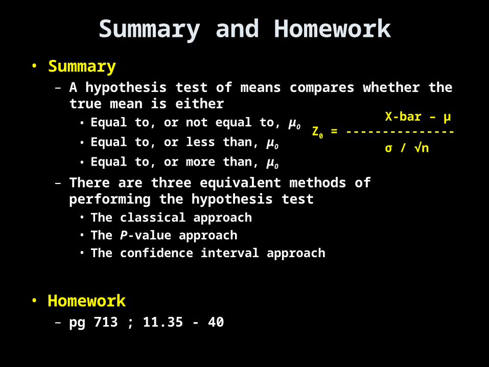
Summary and Homework• Summary

– A hypothesis test of means compares whether the true mean is either• Equal to, or not equal to, μ0

• Equal to, or less than, μ0

• Equal to, or more than, μ0

– There are three equivalent methods of performing the hypothesis test• The classical approach

• The P-value approach

• The confidence interval approach

• Homework– pg 713 ; 11.35 - 40

X-bar – μZ0 = --------------- σ / √n