Lectures on Nuclear and Hadron Physics - UM · Lectures on Nuclear and Hadron Physics Dispersion...
45
Lectures on Nuclear and Hadron Physics Lectures on Nuclear and Hadron Physics J. A. Oller Departamento de F´ ısica Universidad de Murcia July 27, 2011
Transcript of Lectures on Nuclear and Hadron Physics - UM · Lectures on Nuclear and Hadron Physics Dispersion...
Lectures on Nuclear and Hadron Physics
Lectures on Nuclear and Hadron Physics
J. A. Oller
Departamento de FısicaUniversidad de Murcia
July 27, 2011
Lectures on Nuclear and Hadron Physics
Contents
Outline Lecture I
1 Introduction
2 Dispersion Relations
3 S-matrix
4 Scalar Form Factor of the Pion
5 γγ → π0π0
Lectures on Nuclear and Hadron Physics
Contents
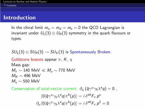
Introduction
In the chiral limit mu = md = ms = 0 the QCD Lagrangian isinvariant under UL(3) ⊗ UR(3) symmetry in the quark flavours ortypes.
SUL(3) ⊗ SUR(3) → SUV (3) is Spontaneously Broken.
Goldstone bosons appear π, K , ηMass gap:Mπ ∼ 140 MeV ≪ Mρ ∼ 770 MeVMK ∼ 496 MeVMη ∼ 550 MeV
Conservation of axial-vector current: ∂µ (qγµγ5λaq) = 0 ,
〈0|qγµγ5λaq|πb(p)〉 = i δabFπ pµ
∂µ〈0|qγµγ5λaq|πb(p)〉 = i δabFπ p2 = 0
Lectures on Nuclear and Hadron Physics
Contents
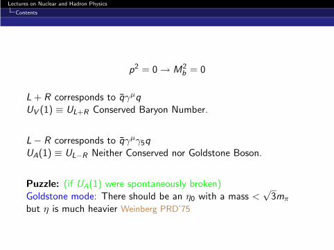
p2 = 0 → M2b = 0
L + R corresponds to qγµqUV (1) ≡ UL+R Conserved Baryon Number.
L − R corresponds to qγµγ5qUA(1) ≡ UL−R Neither Conserved nor Goldstone Boson.
Puzzle: (if UA(1) were spontaneously broken)Goldstone mode: There should be an η0 with a mass <
√3mπ
but η is much heavier Weinberg PRD’75
Lectures on Nuclear and Hadron Physics
Contents
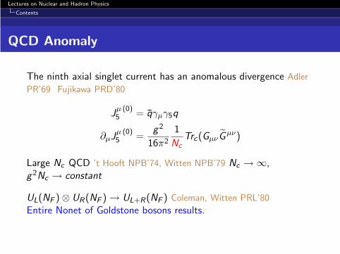
QCD Anomaly
The ninth axial singlet current has an anomalous divergence Adler
PR’69 Fujikawa PRD’80
Jµ (0)5 = qγµγ5q
∂µJµ (0)5 =
g2
16π2
1
Nc
Trc(GµνGµν)
Large Nc QCD ’t Hooft NPB’74, Witten NPB’79 Nc → ∞,g2Nc → constant
UL(NF ) ⊗ UR(NF ) → UL+R(NF ) Coleman, Witten PRL’80
Entire Nonet of Goldstone bosons results.
Lectures on Nuclear and Hadron Physics
Dispersion Relations
Dispersion Relations
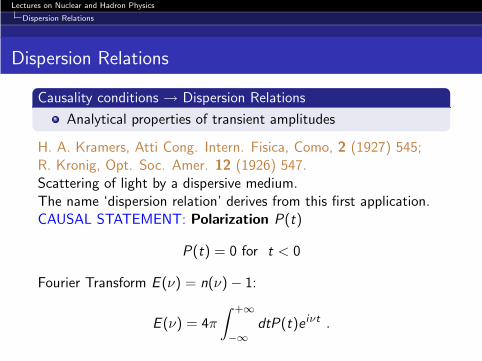
Causality conditions → Dispersion Relations
Analytical properties of transient amplitudes
H. A. Kramers, Atti Cong. Intern. Fisica, Como, 2 (1927) 545;R. Kronig, Opt. Soc. Amer. 12 (1926) 547.Scattering of light by a dispersive medium.The name ‘dispersion relation’ derives from this first application.CAUSAL STATEMENT: Polarization P(t)
P(t) = 0 for t < 0
Fourier Transform E (ν) = n(ν) − 1:
E (ν) = 4π
∫ +∞
−∞
dtP(t)e iνt .
Lectures on Nuclear and Hadron Physics
Dispersion Relations
Dispersion Relation:
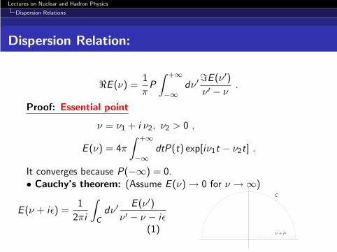
ℜE (ν) =1
πP
∫ +∞
−∞
dν ′ℑE (ν ′)
ν ′ − ν.
Proof: Essential point
ν = ν1 + i ν2, ν2 > 0 ,
E (ν) = 4π
∫ +∞
−∞
dtP(t) exp[iν1t − ν2t] .
It converges because P(−∞) = 0.• Cauchy’s theorem: (Assume E (ν) → 0 for ν → ∞)
E (ν + iǫ) =1
2πi
∫
C
dν ′ E (ν ′)
ν ′ − ν − iǫ(1)
C
ν + iǫ

Lectures on Nuclear and Hadron Physics
Dispersion Relations
0 =1
2πi
∫
C
dν ′ E (ν ′)
ν ′ − ν + iǫ
Complex
Conjugate
→ 0 =1
2πi
∫
C
dν ′ E ∗(ν ′)
ν ′ − ν − iǫ(2)
• Subtracting Eqs.(1), (2):
E (ν) = limǫ→0+
1
π
∫ +∞
−∞
dν ′ ℑE (ν ′)
ν ′ − ν − iǫ(3)
Adding Eqs.(1), (2):
E (ν) = limǫ→0+
−i
π
∫ +∞
−∞
dν ′ ℜE (ν ′)
ν ′ − ν − iǫ(4)
Taking into account
∫ +∞
−∞
dxg(x)
x − x0 ± iǫ= P
∫ +∞
−∞
dxg(x)
x − x0∓ iπg(x0)
Lectures on Nuclear and Hadron Physics
Dispersion Relations
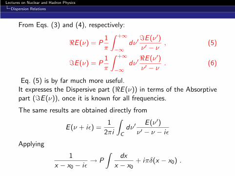
From Eqs. (3) and (4), respectively:
ℜE (ν) = P1
π
∫ +∞
−∞
dν ′ℑE (ν ′)
ν ′ − ν, (5)
ℑE (ν) = P1
π
∫ +∞
−∞
dν ′ℜE (ν ′)
ν ′ − ν. (6)
Eq. (5) is by far much more useful.It expresses the Dispersive part (ℜE (ν)) in terms of the Absorptivepart (ℑE (ν)), once it is known for all frequencies.
The same results are obtained directly from
E (ν + iǫ) =1
2πi
∫
C
dν ′ E (ν ′)
ν ′ − ν − iǫ
Applying
1
x − x0 − iǫ→ P
∫dx
x − x0+ iπδ(x − x0) .
Lectures on Nuclear and Hadron Physics
Dispersion Relations
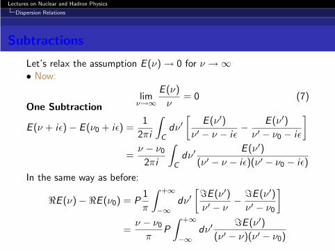
Subtractions
Let’s relax the assumption E (ν) → 0 for ν → ∞• Now:
limν→∞
E (ν)
ν= 0 (7)
One Subtraction
E (ν + iǫ) − E (ν0 + iǫ) =1
2πi
∫
C
dν ′
[E (ν ′)
ν ′ − ν − iǫ− E (ν ′)
ν ′ − ν0 − iǫ
]
=ν − ν0
2πi
∫
C
dν ′ E (ν ′)
(ν ′ − ν − iǫ)(ν ′ − ν0 − iǫ)
In the same way as before:
ℜE (ν) −ℜE (ν0) = P1
π
∫ +∞
−∞
dν ′
[ℑE (ν ′)
ν ′ − ν− ℑE (ν ′)
ν ′ − ν0
]
=ν − ν0
πP
∫ +∞
−∞
dν ′ ℑE (ν ′)
(ν ′ − ν)(ν ′ − ν0)
Lectures on Nuclear and Hadron Physics
Dispersion Relations
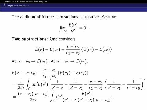
The addition of further subtractions is iterative. Assume:
limν→∞
E (ν)
ν2= 0 .
Two subtractions: One considers
E (ν) − E (ν0) −ν − ν0
ν1 − ν0E (ν1) − E (ν0)
At ν = ν0 → E (ν0). At ν = ν1 → E (ν1).
E (ν) − E (ν0) −ν − ν0
ν1 − ν0E (ν1) − E (ν0)
=1
2πi
∫
C
dν ′E (ν ′)
[1
ν ′ − ν− 1
ν ′ − ν0− ν − ν0
ν1 − ν0
(1
ν ′ − ν1− 1
ν ′ − ν0
)]
=(ν − ν0)(ν − ν1)
2πi
∫
C
dν ′ E (ν ′)
(ν ′ − ν)(ν ′ − ν0)(ν ′ − ν1).
Lectures on Nuclear and Hadron Physics
Dispersion Relations
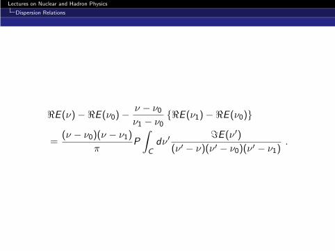
ℜE (ν) −ℜE (ν0) −ν − ν0
ν1 − ν0ℜE (ν1) −ℜE (ν0)
=(ν − ν0)(ν − ν1)
πP
∫
C
dν ′ ℑE (ν ′)
(ν ′ − ν)(ν ′ − ν0)(ν ′ − ν1).
Lectures on Nuclear and Hadron Physics
Dispersion Relations
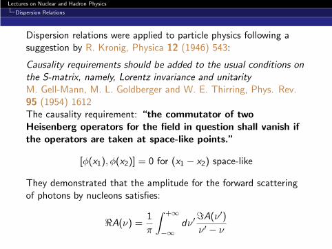
Dispersion relations were applied to particle physics following asuggestion by R. Kronig, Physica 12 (1946) 543:
Causality requirements should be added to the usual conditions onthe S-matrix, namely, Lorentz invariance and unitarityM. Gell-Mann, M. L. Goldberger and W. E. Thirring, Phys. Rev.95 (1954) 1612The causality requirement: “the commutator of twoHeisenberg operators for the field in question shall vanish ifthe operators are taken at space-like points.”
[φ(x1), φ(x2)] = 0 for (x1 − x2) space-like
They demonstrated that the amplitude for the forward scatteringof photons by nucleons satisfies:
ℜA(ν) =1
π
∫ +∞
−∞
dν ′ℑA(ν ′)
ν ′ − ν
Lectures on Nuclear and Hadron Physics
S-matrix
S-matrix
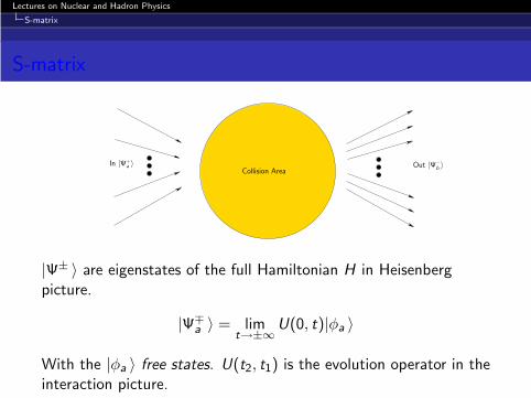
Collision AreaIn |Ψ+
a 〉 Out |Ψ−b 〉
|Ψ± 〉 are eigenstates of the full Hamiltonian H in Heisenbergpicture.
|Ψ∓a 〉 = lim
t→±∞U(0, t)|φa 〉
With the |φa 〉 free states. U(t2, t1) is the evolution operator in theinteraction picture.
Lectures on Nuclear and Hadron Physics
S-matrix
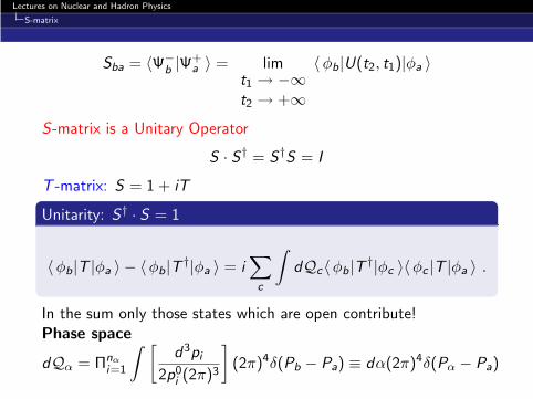
Sba = 〈Ψ−b |Ψ+
a 〉 = limt1 → −∞t2 → +∞
〈φb|U(t2, t1)|φa 〉
S-matrix is a Unitary Operator
S · S† = S†S = I
T -matrix: S = 1 + iT
Unitarity: S† · S = 1
〈φb|T |φa 〉 − 〈φb|T †|φa 〉 = i∑
c
∫dQc〈φb|T †|φc 〉〈φc |T |φa 〉 .
In the sum only those states which are open contribute!Phase space
dQα = Πnα
i=1
∫ [d3pi
2p0i (2π)3
](2π)4δ(Pb − Pa) ≡ dα(2π)4δ(Pα − Pa)
Lectures on Nuclear and Hadron Physics
S-matrix
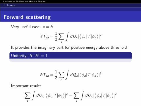
Forward scattering
Very useful case: a = b
ℑTaa =1
2
∑
c
∫dQc |〈φc |T |φa 〉|2
It provides the imaginary part for positive energy above threshold
Unitarity: S · S† = 1
ℑTaa =1
2
∑
c
∫dQc |〈φa|T |φc 〉|2
Important result:
∑
c
∫dQc |〈φc |T |φa 〉|2 =
∑
c
∫dQc |〈φa|T |φc 〉|2
Lectures on Nuclear and Hadron Physics
S-matrix
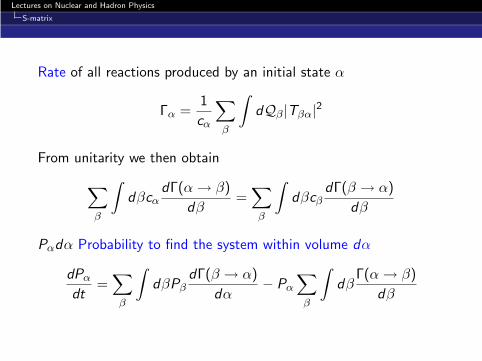
Rate of all reactions produced by an initial state α
Γα =1
cα
∑
β
∫dQβ |Tβα|2
From unitarity we then obtain
∑
β
∫dβcα
dΓ(α → β)
dβ=
∑
β
∫dβcβ
dΓ(β → α)
dβ
Pαdα Probability to find the system within volume dα
dPα
dt=
∑
β
∫dβPβ
dΓ(β → α)
dα− Pα
∑
β
∫dβ
Γ(α → β)
dβ
Lectures on Nuclear and Hadron Physics
S-matrix
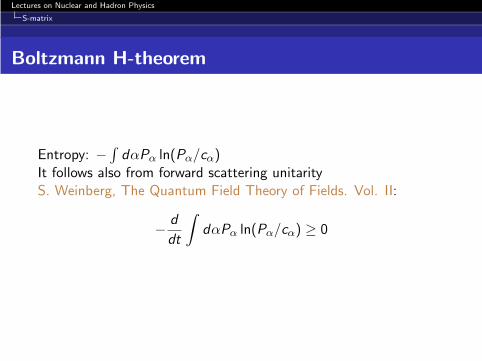
Boltzmann H-theorem
Entropy: −∫
dαPα ln(Pα/cα)It follows also from forward scattering unitarityS. Weinberg, The Quantum Field Theory of Fields. Vol. II:
− d
dt
∫dαPα ln(Pα/cα) ≥ 0
Lectures on Nuclear and Hadron Physics
S-matrix
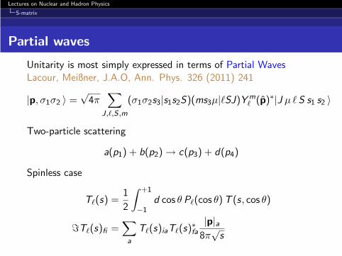
Partial waves
Unitarity is most simply expressed in terms of Partial WavesLacour, Meißner, J.A.O, Ann. Phys. 326 (2011) 241
|p, σ1σ2 〉 =√
4π∑
J,ℓ,S ,m
(σ1σ2s3|s1s2S)(ms3µ|ℓSJ)Y mℓ (p)∗|J µ ℓS s1 s2 〉
Two-particle scattering
a(p1) + b(p2) → c(p3) + d(p4)
Spinless case
Tℓ(s) =1
2
∫ +1
−1d cos θ Pℓ(cos θ)T (s, cos θ)
ℑTℓ(s)fi =∑
a
Tℓ(s)iaTℓ(s)∗fa
|p|a8π
√s
Lectures on Nuclear and Hadron Physics
S-matrix
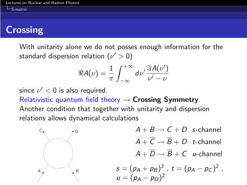
Crossing
With unitarity alone we do not posses enough information for thestandard dispersion relation (ν ′ > 0)
ℜA(ν) =1
π
∫ +∞
−∞
dν ′ℑA(ν ′)
ν ′ − ν
since ν ′ < 0 is also required.Relativistic quantum field theory → Crossing Symmetry.Another condition that together with unitarity and dispersionrelations allows dynamical calculations
A B
C D A + B → C + D s-channel
A + C → B + D t-channel
A + D → B + C u-channel
s = (pA + pB)2 , t = (pA − pC )2 ,u = (pA − pD)2

Lectures on Nuclear and Hadron Physics
S-matrix
Mandelstam Variables: Only two are independents + t + u = m2
A + m2B + m2
C + m2D
A(pA) + B(pB) → C (pC ) + D(pD) s-channel
A(pA) + C (−pC ) → B(−pB) + D(pD) t-channel
A(pA) + D(−pD) → B(−pB) + C (pC ) u-channel
Particle→Antiparticle and reverse four-momentumThe amplitudes for the three reactions are given by the sameanalytic functionPhysical processes correspond to certain values of s, t(disconnected physical regions)
Lectures on Nuclear and Hadron Physics
S-matrix
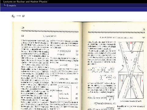
sc → u
III
III
Lectures on Nuclear and Hadron Physics
S-matrix
E.g.
Nπ0 → Nπ0
s- and u-channel processes are the sameFor forward scattering:
ℜA(−ν) = ℜA(ν)
ℑA(−ν) = −ℑA(ν)ℜA(ν) =
∫ +∞
−∞
dν ′ℑA(ν ′)
ν ′ − ν
We have the needed information to apply the dispersion relationν ′ ∈] −∞,−mπ] and [mπ, +∞]
Additionally one also has the one-nucleon pole
g2
2mN
1
ν − m2π/(2mN)
Lectures on Nuclear and Hadron Physics
S-matrix
The application of crossing is not always so straightforward forobtaining the input in the dispersion relation.
Typical example is fixed t dispersion relations
t = −2q2(1 − cos θ)
q2 =(s ′ − (mN + mπ)2)(s ′ − (mN − mπ)2)
4s ′
As s ′ moves as integration variable cos θ will be less than −1 forq2 → 0 (near threshold)
The extension to unphysical values of cos θ can be done makinguse of the partial wave expansion.
However, its convergence its restricted to the Lehmann ellipseH. Lehmann, Nuovo Cim. Suppl. 14 (1959) 153
Lectures on Nuclear and Hadron Physics
S-matrix
πN scattering0 < −t <
32
3
2mN + mπ
2mN − mπm2
π ∼ 32
3m2
π

Lectures on Nuclear and Hadron Physics
S-matrix
The principle of Maximum Analyticity
S. Mandelstam, Rep. Prog. Phys. 25 (1962) 99“The scattering amplitude is analytic in all its variablesexcept at those points where singularities arise as aconsequence of the unitarity condition.” (including thecrossed channels.)This is fulfilled to all orders in perturbation theory.
Direct Crossed
Lectures on Nuclear and Hadron Physics
Scalar Form Factor of the Pion
Scalar Form Factor of the Pion
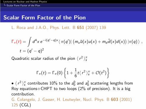
L. Roca and J.A.O., Phys. Lett. B 651 (2007) 139
Γπ(t) =
∫d4x e−i(q′−q)x〈π(q′)|
(muu(x)u(x) + md d(x)d(x)
)|π(q) 〉 , t
t = (q′ − q)2
Quadratic scalar radius of the pion 〈 r2 〉πs
Γπ(t) = Γπ(0)
1 +
1
6t〈 r2 〉πs + O(t2)
• 〈 r2 〉πs contributes 10% to the a00 and a2
0 scattering lengths fromRoy equations+CHPT to two loops (2% of precision). It is a bigcontribution.G. Colangelo, J. Gasser, H. Leutwyler, Nucl. Phys. B 603 (2001)125 (CGL)
Lectures on Nuclear and Hadron Physics
Scalar Form Factor of the Pion
• It gives ℓ4 that controls the departure of Fπ from its value in thechiral limit
〈 r2 〉πs =3
8π2F 2π
(ℓ4 −
13
12
)
Fπ = F
1 +
m2π
16π2F 2π
ℓ4
• Controversy between:The ‘canonical’ value: 〈 r2 〉πs = 0.61 ± 0.04 fm2
Donoghue, Gasser, Leutwyler, Nucl. Phys. B 343 (1990) 341Based on solving the two-channel Muskhelishvili-Omnes equations
F. Yndurain’s approach based on the Omnes representation ofΓπ(t) and high energy QCD behavior〈 r2 〉πs = 0.75 ± 0.07 fm2
Lectures on Nuclear and Hadron Physics
Scalar Form Factor of the Pion
• Change in the ππ scattering lengths:
δa00 = +0.027∆r2 δa2
0 = −0.004∆2r 〈 r2 〉πs = 0.61(1 + ∆2
r ) fm2
∆r2 = +0.23
δa00 = +0.006 δa2
0 = −0.001
CGL:
a00 = 0.220 ± 0.005 a2
0 = −0.0444 ± 0.0010 fm
precision 2%
Lectures on Nuclear and Hadron Physics
Scalar Form Factor of the Pion
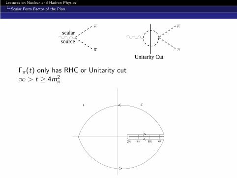
scalar
source
Unitarity Cutreplacements
π
π π
π
Γπ(t) only has RHC or Unitarity cut∞ > t ≥ 4m2
π
2π 4π 6π κκ
t C
Lectures on Nuclear and Hadron Physics
Scalar Form Factor of the Pion
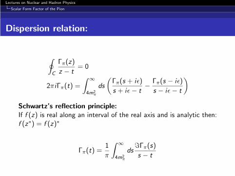
Dispersion relation:
∮
C
Γπ(z)
z − t= 0
2πiΓπ(t) =
∫ ∞
4m2π
ds
(Γπ(s + iǫ)
s + iǫ − t− Γπ(s − iǫ)
s − iǫ − t
)
Schwartz’s reflection principle:If f (z) is real along an interval of the real axis and is analytic then:f (z∗) = f (z)∗
Γπ(t) =1
π
∫ ∞
4m2π
dsℑΓπ(s)
s − t
Lectures on Nuclear and Hadron Physics
Scalar Form Factor of the Pion
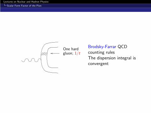
One hardgluon; 1/t
Brodsky-Farrar QCDcounting rulesThe dispersion integral isconvergent

Lectures on Nuclear and Hadron Physics
Scalar Form Factor of the Pion
Omnes representationLet F (t) an analytic function except for the presence of the RHC
1 Remove the zeroes and poles in F (t) in the complex plane
g(t) =F (t)
P(t)
P(t) =F (0)
s1 · · · sn(s1 − t)(s2 − t) · · · (sn − t)
2 Perform a dispersion relation of
f (t) = logF (t)
P(t)
f (t + iǫ) − f (t − iǫ) = logF (t + iǫ)
P(t)− log
F (t − iǫ)
P(t)
= 2i argF (t + iǫ)
P(t)|F (t + iǫ)| = |F (t − iǫ)|
Lectures on Nuclear and Hadron Physics
Scalar Form Factor of the Pion
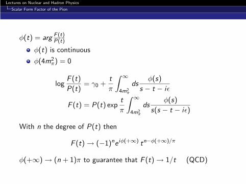
φ(t) = arg F (t)P(t)
φ(t) is continuous
φ(4m2π) = 0
logF (t)
P(t)= γ0 +
t
π
∫ ∞
4m2π
dsφ(s)
s − t − iǫ
F (t) = P(t) expt
π
∫ ∞
4m2π
dsφ(s)
s(s − t − iǫ)
With n the degree of P(t) then
F (t) → (−1)ne iφ(+∞) tn−φ(+∞)/π
φ(+∞) → (n + 1)π to guarantee that F (t) → 1/t (QCD)

Lectures on Nuclear and Hadron Physics
Scalar Form Factor of the Pion
Watson final state theorem
S = 1 + i2ρ(F + T )
SS† = 1
• Elastic case (only ππ intermediate state)• Keep only linear terms in F . There is only one source!
ℑΓπ(t) = Γπ(t)ρ(t)T ∗ππ(t)
Since the ℑΓπ(t) is real the phase of F (t) (φ(t)) and of Tππ(t)(δ(t)) are the same (modulo π)

Lectures on Nuclear and Hadron Physics
Scalar Form Factor of the Pion
Corolary
tππ = ρTππ = sin δπ e iδπ , δπ(4m2π) = 0, δπ is continuous and at
most differs by modulo π from the phase of Tππ
This happens when δπ crosses π (sin δπ < 0)
F (t) = P(t) exp1
π
∫ ∞
4m2π
dsφ(s)
s(s − t)
φ(s) = δ(s) s < 4m2K
Lectures on Nuclear and Hadron Physics
Scalar Form Factor of the Pion
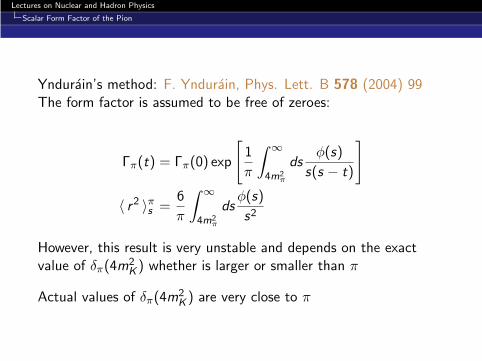
Yndurain’s method: F. Yndurain, Phys. Lett. B 578 (2004) 99The form factor is assumed to be free of zeroes:
Γπ(t) = Γπ(0) exp
[1
π
∫ ∞
4m2π
dsφ(s)
s(s − t)
]
〈 r2 〉πs =6
π
∫ ∞
4m2π
dsφ(s)
s2
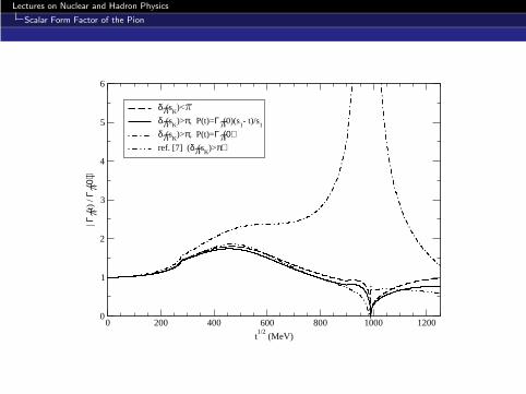
However, this result is very unstable and depends on the exactvalue of δπ(4m2
K ) whether is larger or smaller than π
Actual values of δπ(4m2K ) are very close to π
Lectures on Nuclear and Hadron Physics
Scalar Form Factor of the Pion
0 200 400 600 800 1000 1200
t1/2
(MeV)
0
1
2
3
4
5
6| Γ
(t)
/ Γ(0
) |
δ (sK
)<
δ (sK
)>π, P(t)=Γ (0)(s1- t)/s
1
δ (sK
)>π, P(t)=Γ (0)ref. [7] (δ (s
K)>π)π
ππππ
ππ
ππ
Lectures on Nuclear and Hadron Physics
Scalar Form Factor of the Pion
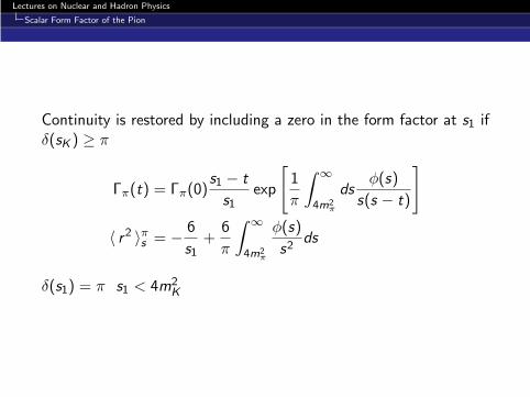
Continuity is restored by including a zero in the form factor at s1 ifδ(sK ) ≥ π
Γπ(t) = Γπ(0)s1 − t
s1exp
[1
π
∫ ∞
4m2π
dsφ(s)
s(s − t)
]
〈 r2 〉πs = − 6
s1+
6
π
∫ ∞
4m2π
φ(s)
s2ds
δ(s1) = π s1 < 4m2K
Lectures on Nuclear and Hadron Physics
Scalar Form Factor of the Pion
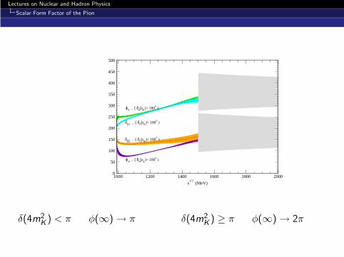
1000 1200 1400 1600 1800 2000
s1/2
(MeV)
0
50
100
150
200
250
300
350
400
450
500
ϕπ , ( δπ(sK)< 180
o )
δ(+) , ( δπ(sK)< 180
o )
ϕπ , ( δπ(sK)> 180
o )
δ(+) , ( δπ(sK)> 180
o )
δ(4m2K ) < π φ(∞) → π δ(4m2
K ) ≥ π φ(∞) → 2π
Lectures on Nuclear and Hadron Physics
Scalar Form Factor of the Pion
φas ≃ π
(n ± 2dm
log(s/Λ2)
)
dm = 12/(33 − 2nf ) ≃ 1/2Λ is the scale QCD parametern = 1, 2 for δπ(4m2
K ) < π, ≥ π
〈 r2 〉πs = 0.63 ± 0.05 fm2
Compatible with CGL 〈 r2 〉πs = 0.61 ± 0.04 fm2
Both methods are compatible
Lectures on Nuclear and Hadron Physics
γγ → π0π
0
γγ → π0π0
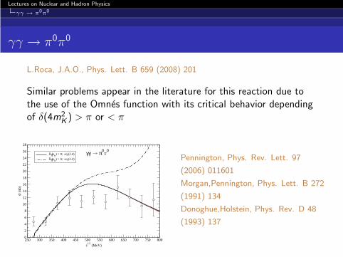
L.Roca, J.A.O., Phys. Lett. B 659 (2008) 201
Similar problems appear in the literature for this reaction due tothe use of the Omnes function with its critical behavior dependingof δ(4m2
K ) > π or < π
250 300 350 400 450 500 550 600 650 700 750 800
s1/2
(MeV)
0
2
4
6
8
10
12
14
16
18
20
22
24
26
28
σ (n
b)
δ (sK
) > π, eq.(2.4)
δ (sK
) > π, eq.(2.2)
γγ π0 0π
ππ Pennington, Phys. Rev. Lett. 97
(2006) 011601
Morgan,Pennington, Phys. Lett. B 272
(1991) 134
Donoghue,Holstein, Phys. Rev. D 48
(1993) 137

Lectures on Nuclear and Hadron Physics
γγ → π0π
0
The amplitude F (s) has RHC and LHC. The latter is given by L(s)
F (s) − L(s)
has only RHC
Ω(s) =
(1 − θ(s1)
s
s1
)exp
[s
π
∫ ∞
4m2π
φ0(s′)
s ′(s ′ − s)ds ′
]
Twice-subtracted dispersion relation for
(F (s) − L(s))/Ω(s)
F (s) = L(s) + c0sΩ(s) +s2
πΩ(s)
∫ ∞
4m2π
L0(s′) sin φ0(s
′)
s ′2(s ′ − s)|Ω(s ′)|ds ′
+ θ(s1 − 4m2K )
Ω0(s)
Ω0(s1)
s2
s21
(F0(s1) − L0(s1)) .
Lectures on Nuclear and Hadron Physics
γγ → π0π
0
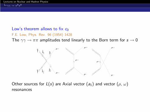
Low’s theorem allows to fix c0
F.E. Low, Phys. Rev. 96 (1954) 1428
The γγ → ππ amplitudes tend linearly to the Born term for s → 0
P
p 1
p 2k 2
k 1
P
γ
γ
P
P
P+
P+
P+
P+
P−
P−P−
P−
Other sources for L(s) are Axial vector (a1) and vector (ρ, ω)resonances
Lectures on Nuclear and Hadron Physics
γγ → π0π
0
250 300 350 400 450 500 550 600 650 700 750 800
s1/2
(MeV)
0
4
8
12
16
20
σ (n
b)
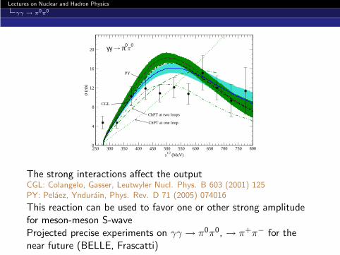
γγ π0 0
ChPT at two loops
PY
CGL
ChPT at one loop
π
The strong interactions affect the outputCGL: Colangelo, Gasser, Leutwyler Nucl. Phys. B 603 (2001) 125PY: Pelaez, Yndurain, Phys. Rev. D 71 (2005) 074016
This reaction can be used to favor one or other strong amplitudefor meson-meson S-waveProjected precise experiments on γγ → π0π0, → π+π− for thenear future (BELLE, Frascatti)