Lectures on CMB Obervation : Part IScientific goals and observational

techniques

Martin Bucher, APC Paris, Kyoto, Japan, March 2010

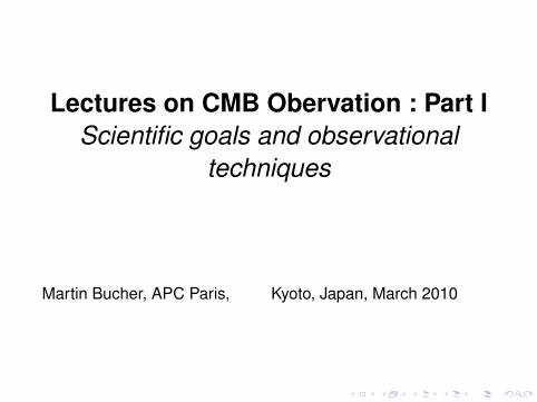
WMAP Internal Linear Combination (ILC) Map

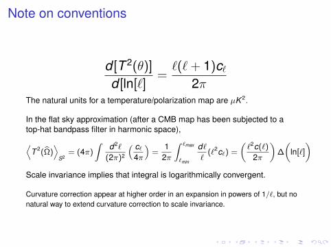
Note on conventions

d [T 2(θ)]

d [ln[`]=`(`+ 1)c`

2πThe natural units for a temperature/polarization map are µK 2.

In the flat sky approximation (after a CMB map has been subjected to atop-hat bandpass filter in harmonic space),D

T 2(bΩ)E

S2= (4π)

Zd2`

(2π)2

“ c`4π

”=

12π

Z `max

`min

d``

(`2c`) =

„`2c(`)

2π

«∆

„ln[`]

«Scale invariance implies that integral is logarithmically convergent.

Curvature correction appear at higher order in an expansion in powers of 1/`, but nonatural way to extend curvature correction to scale invariance.

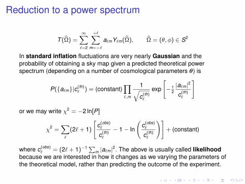
Reduction to a power spectrum

T (bΩ) =∞X`=2

+Xm=−`

a`mY`m(bΩ), bΩ = (θ, φ) ∈ S2

In standard inflation fluctuations are very nearly Gaussian and theprobability of obtaining a sky map given a predicted theoretical powerspectrum (depending on a number of cosmological parameters θ) is

P(a`m|c(th)` ) = (constant)

Y`,m

1qc(th)`

exp

"− 1

2|a`m|2

c(th)`

#

or we may write χ2 = −2 ln[P]

χ2 =X`

(2`+ 1)

"c(obs)`

c(th)`

− 1− ln

c(obs)`

c(th)`

!#+ (constant)

where c(obs)` = (2`+ 1)−1P

m |a`m|2. The above is usually called likelihood

because we are interested in how it changes as we varying the parameters ofthe theoretical model, rather than predicting the outcome of the experiment.

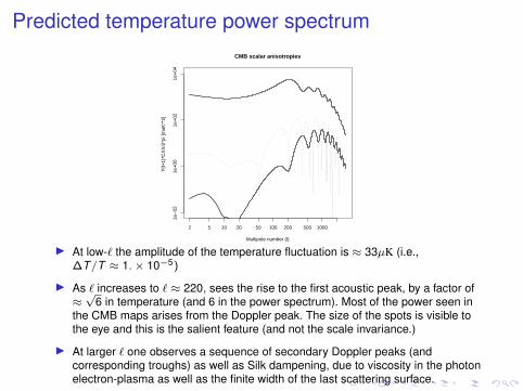
Predicted temperature power spectrum

2 5 10 20 50 100 200 500 1000

1e−

021e

+00

1e+

021e

+04

CMB scalar anisotropies

Multipole number (l)

l*(l+

1)*C

XX

/2*p

i [m

uK**

2]

I At low-` the amplitude of the temperature fluctuation is ≈ 33µK (i.e.,∆T/T ≈ 1.× 10−5)

I As ` increases to ` ≈ 220, sees the rise to the first acoustic peak, by a factor of≈√

6 in temperature (and 6 in the power spectrum). Most of the power seen inthe CMB maps arises from the Doppler peak. The size of the spots is visible tothe eye and this is the salient feature (and not the scale invariance.)

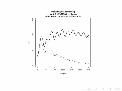
I At larger ` one observes a sequence of secondary Doppler peaks (andcorresponding troughs) as well as Silk dampening, due to viscosity in the photonelectron-plasma as well as the finite width of the last scattering surface.

Including instrument noise (and incomplete skycoverage)

χ2 = T Tsky (C + N)−1Tsky + log[det(Cth + N)]

In general, noise is assumed (to a first approximation) uncorrelated betweenpixels but not necessarily uniform on the sky. Therefore, the N no longertakes the simple form

N`m;`′m′ = N`δ``′δmm′

N`m;`′m′ = (constant)(1/√

t)`m(1/√

t)`′m′

or even a less restricted form when non-whiteness (i.e., redness) of the noiseis allowed.Warning : Although the above defines an exact representation of thelikelihood, given the large number of pixels present, evaluating the above isnot feasible, at least on all scales, and much work has gone into developinggood approximations to the likelihood that are fast to compute. (If Npix = 106

for example, N3pix = 1018 operations are required to invert a matrix.)

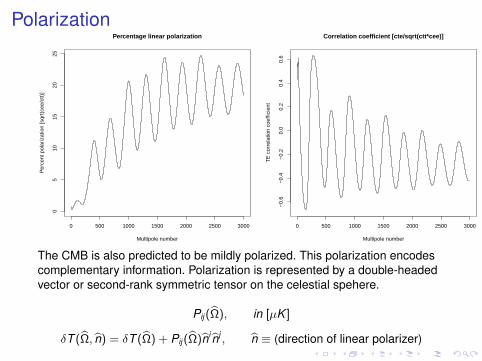
Polarization

0 500 1000 1500 2000 2500 3000

05

1015

2025

Percentage linear polarization

Multipole number

Per

cent

pol

ariz

atio

n [s

qrt(

cee/

ctt)

]

0 500 1000 1500 2000 2500 3000

−0.

6−

0.4

−0.

20.

00.

20.

40.

6

Correlation coefficient [cte/sqrt(ctt*cee)]

Multipole number

TE

cor

rela

tion

coef

ficie

nt

The CMB is also predicted to be mildly polarized. This polarization encodescomplementary information. Polarization is represented by a double-headedvector or second-rank symmetric tensor on the celestial spehere.

Pij (bΩ), in [µK ]

δT (bΩ, bn) = δT (bΩ) + Pij (bΩ)bnibnj , bn ≡ (direction of linear polarizer)

Scalar and Tensor CMB Anisotropies with PLANCK

Red=scalar (top to bottom) TT, TE, EE, BB (lensing)Blue=tensor (T/S=0.1) = TT, TE, EE, BB, dotted BB (T/S=0.01, 0.001)Green PLANCK capabilities = top single alm, bottom agressive binning

0 500 1000 1500 2000 2500 3000

050

100

150

Illustrating Silk dampening sqrt(l*(l+1)*cTT/2.pi) −− dotted,

sqrt(l*(l+1)*cTT/2.pi)*exp(l/1000.) −− solid

Multipole

muK

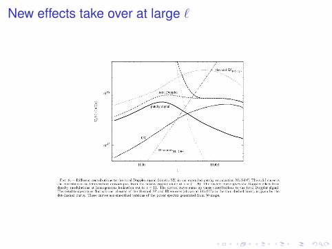
New effects take over at large `

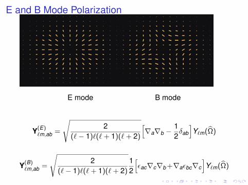
E and B Mode Polarization

E mode B mode

Y(E)`m,ab =

√2

(`− 1)`(`+ 1)(`+ 2)

[∇a∇b −

12δab

]Y`m(Ω)

Y(B)`m,ab =

√2

(`− 1)`(`+ 1)(`+ 2)

12

[εac∇c∇b +∇aεbc∇c

]Y`m(Ω)

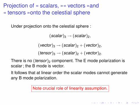
Projection of « scalars, »« vectors »and« tensors »onto the celestial sphere

Under projection onto the celestial sphere :

(scalar)3 → (scalar)2,

(vector)3 → (scalar)2 + (vector)2,

(tensor)3 → (scalar)2 + (vector)2.

There is no (tensor)2 component. The E mode polarization isscalar ; the B mode is vector.

It follows that at linear order the scalar modes cannot generateany B mode polarization.

Note crucial role of linearity assumption.

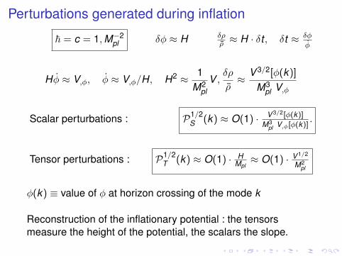
Perturbations generated during inflation

~ = c = 1,M−2pl δφ ≈ H δρ

ρ ≈ H · δt , δt ≈ δφ

φ

Hφ ≈ V,φ, φ ≈ V,φ/H, H2 ≈ 1M2

plV ,

δρ

ρ≈ V 3/2[φ(k)]

M3pl V,φ

Scalar perturbations : P1/2S (k) ≈ O(1) · V 3/2[φ(k)]

M3pl V,φ[φ(k)]

.

Tensor perturbations : P1/2T (k) ≈ O(1) · H

Mpl≈ O(1) · V 1/2

M2pl

φ(k) ≡ value of φ at horizon crossing of the mode k

Reconstruction of the inflationary potential : the tensorsmeasure the height of the potential, the scalars the slope.

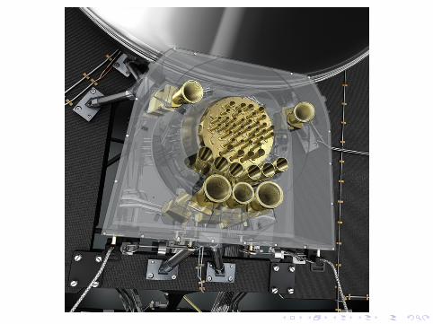
Technologies for the detecting CMB fluctuations

Two competing photon detection strategies

I Coherent detectors — Basically high-sensitivity, low-noise radio setsused to amplify and then measure the incoming CMB signal.Advantages : Can be operated in space with passive cooling. Noisetemperature is less than the ambient temperature. Disadvantages : Atpresent more noisy than bolometers and do not extend above 100 GHzfor CMB applications.

I Incoherent (“bolometric”) detectors — Incoming photons heat device, alarge number of smaller energy quasi-particle excitations thatthermalize. Signal is temperature of the detector may be regarded as aclassical observable because of the large number of quanta into whicheach incoming photon is converted. At present, mainly used at highfrequencies ν >∼ 100GHz, but no obstacle (other than low power fluxes)to using bolometers at lower frequencies.Advantages : Very sensitive, almost at the quantum limit due tounavoidable photon shot noise. Very important for space, less importantfrom the ground where atmospheric noise dominates over CMB shotnoise. Disadvantages : Require very low temperatures ≈ 0.1 If coolingfails, data is unusable.

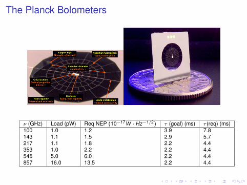
The Planck Bolometers

ν (GHz) Load (pW) Req NEP (10−17W · Hz−1/2) τ (goal) (ms) τ (req) (ms)100 1.0 1.2 3.9 7.8143 1.1 1.5 2.9 5.7217 1.1 1.8 2.2 4.4353 1.0 2.2 2.2 4.4545 5.0 6.0 2.2 4.4857 16.0 13.5 2.2 4.4

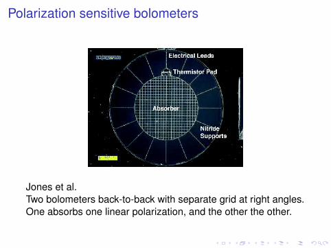
Polarization sensitive bolometers

Jones et al.Two bolometers back-to-back with separate grid at right angles.One absorbs one linear polarization, and the other the other.

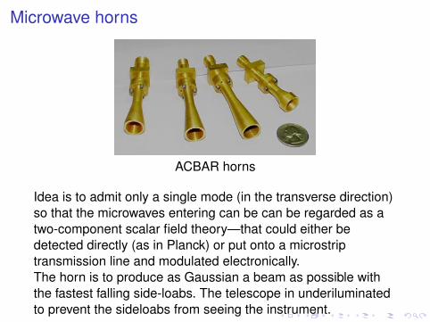
Microwave horns

ACBAR horns

Idea is to admit only a single mode (in the transverse direction)so that the microwaves entering can be can be regarded as atwo-component scalar field theory—that could either bedetected directly (as in Planck) or put onto a microstriptransmission line and modulated electronically.The horn is to produce as Gaussian a beam as possible withthe fastest falling side-loabs. The telescope in underiluminatedto prevent the sideloabs from seeing the instrument.

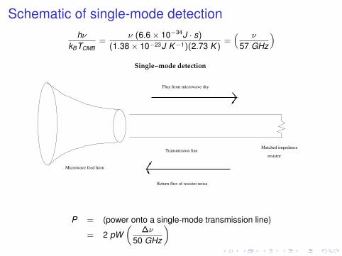
Schematic of single-mode detectionhν

kBTCMB=

ν (6.6× 10−34J · s)

(1.38× 10−23J K−1)(2.73 K )=“ ν

57 GHz

”

Microwave feed horn

Transmission lineMatched impedance

resistor

Flux from microwave sky

Return flux of resistor noise

Single−mode detection

P = (power onto a single-mode transmission line)

= 2 pW„

∆ν

50 GHz

«

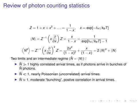
Review of photon counting statistics

Z = 1 + x + x2 + . . . =1

1− x, x = exp[−~ω/kBT ]

〈N〉 = Z−1„

x∂

∂x

«Z =

x1− x

=1

exp[~ω/kBT ]− 1DN2E

= Z−1„

x∂

∂x

«2

Z =2x2

(1− x)2 +x

(1− x)= 2 〈N〉2 + 〈N〉

Two limits and an intermediate regime (N = 〈N〉) :I N 1 highly correlated arrival times, as if photons arrive in bunches of

N photons.I N 1, nearly Poissonian (uncorrelated) arrival times.I N ≈ 1, moderate “bunching”, postive correlation in arrival times.

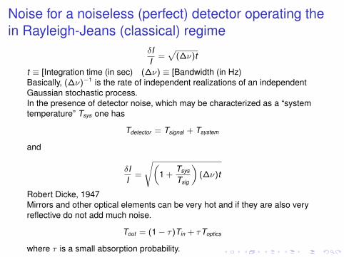
Noise for a noiseless (perfect) detector operating thein Rayleigh-Jeans (classical) regime

δII

=p

(∆ν)t

t ≡ [Integration time (in sec) (∆ν) ≡ [Bandwidth (in Hz)Basically, (∆ν)−1 is the rate of independent realizations of an independentGaussian stochastic process.In the presence of detector noise, which may be characterized as a “systemtemperature” Tsys one has

Tdetector = Tsignal + Tsystem

and

δII

=

s„1 +

Tsys

Tsig

«(∆ν)t

Robert Dicke, 1947Mirrors and other optical elements can be very hot and if they are also veryreflective do not add much noise.

Tout = (1− τ)Tin + τToptics

where τ is a small absorption probability.

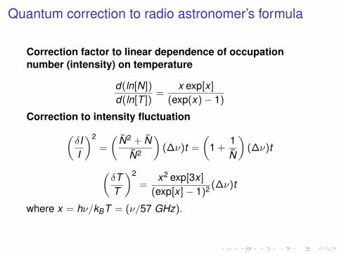
Quantum correction to radio astronomer’s formula

Correction factor to linear dependence of occupationnumber (intensity) on temperature

d(ln[N])

d(ln[T ])=

x exp[x ]

(exp(x)− 1)

Correction to intensity fluctuation(δII

)2

=

(N2 + N

N2

)(∆ν)t =

(1 +

1N

)(∆ν)t

(δTT

)2

=x2 exp[3x ]

(exp[x ]− 1)2 (∆ν)t

where x = hν/kBT = (ν/57 GHz).

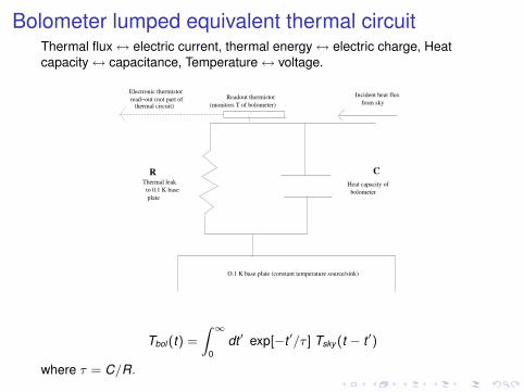
Bolometer lumped equivalent thermal circuitThermal flux↔ electric current, thermal energy↔ electric charge, Heatcapacity↔ capacitance, Temperature↔ voltage.

C

Incident heat flux

from sky

Heat capacity of

bolometer

R

Thermal leak

to 0.1 K base

plate

O.1 K base plate (constant temperature source/sink)

Readout thermistor

(monitors T of bolometer)

Electronic thermistor

read−out (not part ofthermal circuit)

Tbol (t) =

Z ∞0

dt ′ exp[−t ′/τ ] Tsky (t − t ′)

where τ = C/R.

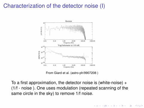
Characterization of the detector noise (I)

Resistor

0.01 0.10 1.00 10.00 100.00 1000.00Frequency (Hz)

1

10

(nV

/Hz^

0.5)

Yogi bolometer at 110 mK

0.01 0.10 1.00 10.00 100.00 1000.00Frequency (Hz)

10-18

10-17

10-16

10-15

(W

/Hz^

0.5)

From Giard et al. (astro-ph/9907208 )

To a first approximation, the detector noise is (white-noise) +(1/f - noise ). One uses modulation (repeated scanning of thesame circle in the sky) to remove 1/f noise.

Characterization of the detector noise (II)As a first approximation, one assumes that detector noise in a sky map isuncorrelated between pixels with variance inversely proportional to the pixelintegration time.

For equal integration time for each pixel

N` = N0

(i.e., a “white-noise” spectrum, rather than the very “red” approximatelyscale-invariant CMB spectrum c` ∝ `−2.)

Non-uniform sky coverage, let t(bΩ) be the integration time in the Ω directionand expand

t1/2(bΩ) = t1/2`mY`m

(summation implied). Then

(N−1)`,m;`′,m′ = t1/2∗`mt1/2

`′m′

(Note that if sky coverage is incomplete N−1 is well-defined, but its inverse Nis not.)

Accounting for the finite-width beam profile

To a first approximation we assume that the beam profile is Gaussian and theaxially symmetric

Tobserved (bΩ) =

Zd bΩ′ K

“Θ(bΩ; bΩ′)” Tsky (bΩ′)

≈ 12πσ2

beam

Zd bΩ′ exp

»− Θ2

2σ2beam

–Tsky (bΩ′)

K acts as a low-pass smoothing filter. In harmonic space

a(map)`m = exp[− 1

2 (`σbeam)2] · a(sky)`m = exp[− 1

2 (`/`beam)2] · a(sky)`m

Note that θbeam = `beam−1 = θFWHM

beam /p

8 log(2) so that

`beam = 1460ׄ

θFWHMbeam

1 arcmin

«FWHM = full width half maximum

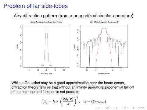
Problem of far side-lobes

Airy diffraction pattern (from a unapodized circular aperature)

−20 −10 0 10 20

0.0

0.2

0.4

0.6

0.8

1.0

Airy diffraction pattern (logarithmic scale)

theta/sigma_theta

Inte

nsity

−20 −10 0 10 20

1e−

091e

−07

1e−

051e

−03

1e−

01

Airy diffraction pattern (linear scale)

theta/sigma_thetaIn

tens

ity

While a Gaussian may be a good approximation near the beam center,diffraction theory tells us that without an infinite aperature exponential fall-offof the point spread function is not possible.

I(x) = I0 ׄ

2J1(x)

x

«2

, x = (θ/θbeam)

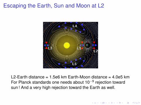
Escaping the Earth, Sun and Moon at L2

L2-Earth distance = 1.5e6 km Earth-Moon distance = 4.0e5 kmFor Planck standards one needs about 10−9 rejection towardsun ! And a very high rejection toward the Earth as well.

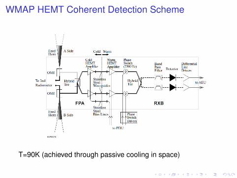
WMAP HEMT Coherent Detection Scheme

T=90K (achieved through passive cooling in space)

WMAP modulation Strategy for overcoming 1/f noise

v1,in =1√2

„A + B√

2+ n1

«g1(t)± 1√

2

„A− B√

2+ n2

«g2(t)

v2,in =1√2

„A + B√

2+ n1

«g1(t)∓ 1√

2

„A− B√

2+ n2

«g2(t)

VL =

„A2 + B2

2+ n2

1

«g1

2(t) +

„A2 + B2

2+ n2

2

«g2

2(t)∓ (A2 − B2)g1(t)g2(t)

VR =

„A2 + B2

2+ n2

1

«g1

2(t) +

„A2 + B2

2+ n2

2

«g2

2(t)± (A2 − B2)g1(t)g2(t)

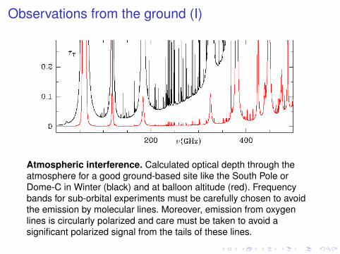
Observations from the ground (I)

Atmospheric interference. Calculated optical depth through theatmosphere for a good ground-based site like the South Pole orDome-C in Winter (black) and at balloon altitude (red). Frequencybands for sub-orbital experiments must be carefully chosen to avoidthe emission by molecular lines. Moreover, emission from oxygenlines is circularly polarized and care must be taken to avoid asignificant polarized signal from the tails of these lines.

Observations from the ground (II)

Numerous CMB polarization experiments from the ground andballoons at various stages : QUaD, BICEP ; BRAIN, CLOVER,EBEx, PAPPA, PolarBear, QUIET and Spider

I Far side lobes

I Scanning strategy (must scan at constant zenith angle)

I Polarization from interaction of Zeeman splitting by earth’smagnetic field of oxgen lines. Atmospheric backscattering(very polarized) could be a serious problem. [SeeL. Pietranera et al., “Observing the CMB polarizationthrough ice,” MNRAS 346, 645 (2007)].

I Lack of stability and partial sky coverage

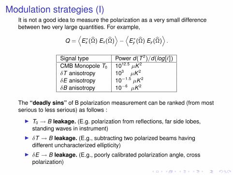
Modulation strategies (I)It is not a good idea to measure the polarization as a very small differencebetween two very large quantities. For example,

Q =D

E∗x (bΩ) Ex (bΩ)E−D

E∗y (bΩ) Ey (bΩ)E.

Signal type Power d(T 2)/d(log[`])

CMB Monopole T0 1012.5 µK 2

δT anisotropy 103 µK 2

δE anisotropy 10−1.5 µK 2

δB anisotropy 10−6 µK 2

The “deadly sins” of B polarization measurement can be ranked (from mostserious to less serious) as follows :

I T0 → B leakage. (E.g. polarization from reflections, far side lobes,standing waves in instrument)

I δT → B leakage. (E.g., subtracting two polarized beams havingdifferent uncharacterized ellipticity)

I δE → B leakage. (E.g., poorly calibrated polarization angle, crosspolarization)

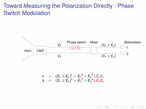
Toward Measuring the Polarization Directly : PhaseSwitch Modulation

Horn OMT

Ex

EyMixer

(Ex ∓ Ey )

(Ex ± Ey )Phase switch

×(±1)

Bolometers

I1

I2

I1 = (Ex ± Ey )2 = Ex2 + Ey

2±Ex Ey

I2 = (Ex ∓ Ey )2 = Ex2 + Ey

2∓Ex Ey

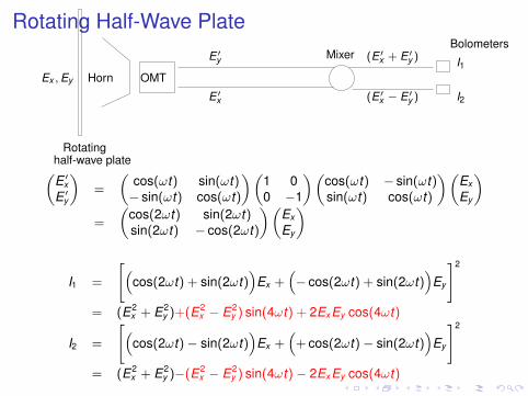
Rotating Half-Wave Plate

Horn OMTEx ,Ey

E ′x

E ′y Mixer

(E ′x − E ′y )

(E ′x + E ′y )Bolometers

I1

I2

Rotatinghalf-wave plate„E ′xE ′y

«=

„cos(ωt) sin(ωt)− sin(ωt) cos(ωt)

«„1 00 −1

«„cos(ωt) − sin(ωt)sin(ωt) cos(ωt)

«„Ex

Ey

«=

„cos(2ωt) sin(2ωt)sin(2ωt) − cos(2ωt)

«„Ex

Ey

«

I1 =

"“cos(2ωt) + sin(2ωt)

”Ex +

“− cos(2ωt) + sin(2ωt)

”Ey

#2

= (E2x + E2

y )+(E2x − E2

y ) sin(4ωt) + 2Ex Ey cos(4ωt)

I2 =

"“cos(2ωt)− sin(2ωt)

”Ex +

“+ cos(2ωt)− sin(2ωt)

”Ey

#2

= (E2x + E2

y )−(E2x − E2

y ) sin(4ωt)− 2Ex Ey cos(4ωt)

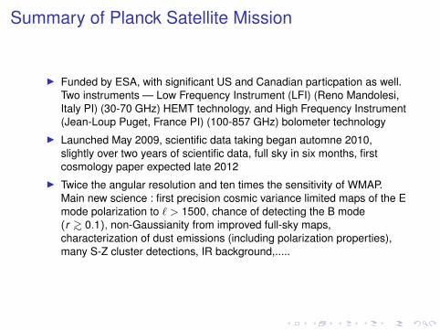
Summary of Planck Satellite Mission

I Funded by ESA, with significant US and Canadian particpation as well.Two instruments — Low Frequency Instrument (LFI) (Reno Mandolesi,Italy PI) (30-70 GHz) HEMT technology, and High Frequency Instrument(Jean-Loup Puget, France PI) (100-857 GHz) bolometer technology

I Launched May 2009, scientific data taking began automne 2010,slightly over two years of scientific data, full sky in six months, firstcosmology paper expected late 2012

I Twice the angular resolution and ten times the sensitivity of WMAP.Main new science : first precision cosmic variance limited maps of the Emode polarization to ` > 1500, chance of detecting the B mode(r >∼ 0.1), non-Gaussianity from improved full-sky maps,characterization of dust emissions (including polarization properties),many S-Z cluster detections, IR background,.....

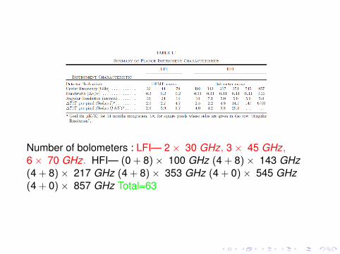
Number of bolometers : LFI— 2× 30 GHz, 3× 45 GHz,6× 70 GHz. HFI— (0 + 8)× 100 GHz (4 + 8)× 143 GHz(4 + 8)× 217 GHz (4 + 8)× 353 GHz (4 + 0)× 545 GHz(4 + 0)× 857 GHz Total=63

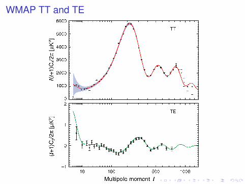
WMAP TT and TE

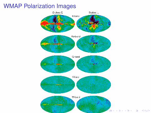
WMAP Polarization Images

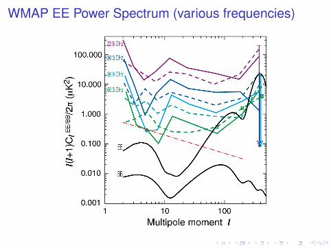
WMAP EE Power Spectrum (various frequencies)

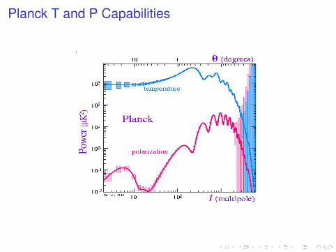
Planck T and P Capabilities

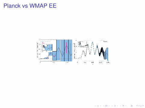
Planck vs WMAP EE

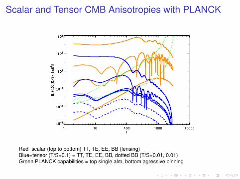
Scalar and Tensor CMB Anisotropies with PLANCK

Red=scalar (top to bottom) TT, TE, EE, BB (lensing)Blue=tensor (T/S=0.1) = TT, TE, EE, BB, dotted BB (T/S=0.01, 0.01)Green PLANCK capabilities = top single alm, bottom agressive binning

Lectures on CMB Obervation : Part IISecondary anisotropies and their

Removal

Martin Bucher, APC Paris, Kyoto, Japan, March 2010

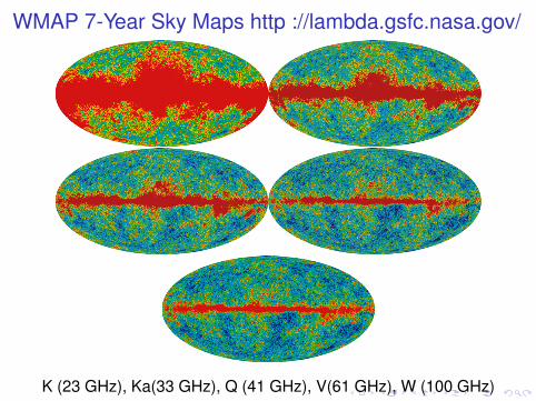
WMAP 7-Year Sky Maps http ://lambda.gsfc.nasa.gov/

K (23 GHz), Ka(33 GHz), Q (41 GHz), V(61 GHz), W (100 GHz)

WMAP Internal Linear Combination (ILC) Map

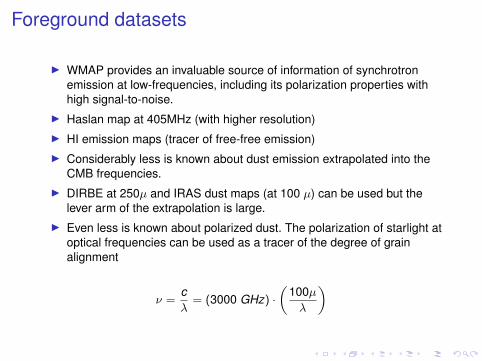
Foreground datasets

I WMAP provides an invaluable source of information of synchrotronemission at low-frequencies, including its polarization properties withhigh signal-to-noise.

I Haslan map at 405MHz (with higher resolution)I HI emission maps (tracer of free-free emission)I Considerably less is known about dust emission extrapolated into the

CMB frequencies.I DIRBE at 250µ and IRAS dust maps (at 100 µ) can be used but the

lever arm of the extrapolation is large.I Even less is known about polarized dust. The polarization of starlight at

optical frequencies can be used as a tracer of the degree of grainalignment

ν =cλ

= (3000 GHz) ·„

100µλ

«

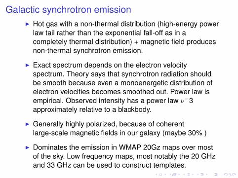
Galactic synchrotron emissionI Hot gas with a non-thermal distribution (high-energy power

law tail rather than the exponential fall-off as in acompletely thermal distribution) + magnetic field producesnon-thermal synchrotron emission.

I Exact spectrum depends on the electron velocityspectrum. Theory says that synchrotron radiation shouldbe smooth because even a monoenergetic distribution ofelectron velocities becomes smoothed out. Power law isempirical. Observed intensity has a power law ν−3approximately relative to a blackbody.

I Generally highly polarized, because of coherentlarge-scale magnetic fields in our galaxy (maybe 30% )

I Dominates the emission in WMAP 20Gz maps over mostof the sky. Low frequency maps, most notably the 20 GHzand 33 GHz can be used to construct templates.

WMAP EE Power Spectrum (various frequencies)

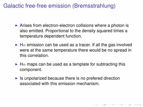
Galactic free-free emission (Bremsstrahlung)

I Arises from electron-electron collisions where a photon isalso emitted. Proportional to the density squared times atemperature dependent function.

I Hα emission can be used as a tracer. If all the gas involvedwere at the same temperature there would be no spread inthis correlation.

I Hα maps can be used as a template for subtracting thiscomponent.

I Is unpolarized because there is no prefered directionassociated with this emission mechanism.

Physics of thermal dust emission

The following simplifications lead to a very simple theoreticaltemplate :

I Dust grains are very small compared to the wavelengths ofinterest

I All resonances of the dust grain coupled to theelectromagnetic field lie at frequencies far above those ofinterest

I The dust is optically thin

Idust (ν,Ω) = τ(Ω; ν0)

(ν

ν0

)2

B(ν,Tdust )

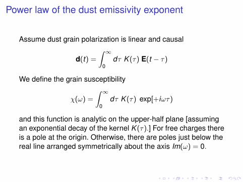
Power law of the dust emissivity exponent

Assume dust grain polarization is linear and causal

d(t) =

∫ ∞0

dτ K (τ) E(t − τ)

We define the grain susceptibility

χ(ω) =

∫ ∞0

dτ K (τ) exp[+iωτ)

and this function is analytic on the upper-half plane [assumingan exponential decay of the kernel K (τ).] For free charges thereis a pole at the origin. Otherwise, there are poles just below thereal line arranged symmetrically about the axis Im(ω) = 0.

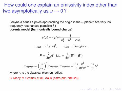
How could one explain an emissivity index other thantwo asymptotically as ω → 0 ?

(Maybe a series a poles approaching the origin in the ω-plane ? Are very lowfrequency resonances plausible ? )Lorentz model (harmonically bound charge)

χ(ω) = (e/m)1

ω20 − ω2 − iγω

σelast = ω4χ(ω)2, σabs = ωIm[χ(ω)],

P =2

3c2 d2,Uinc =1

8π(E2 + B2)

σRayleigh =

„ω

ω0

«4

σThomson, σThomson =8π3

e4

m2c4 =8π3

re2

where re is the classical electron radius.

C. Meny, V. Gromov et al., A& A (astro-ph/0701226)

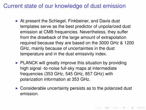
Current state of our knowledge of dust emission

I At present the Schlegel, Finkbeiner, and Davis dusttemplates serve as the best predictor of unpolarized dustemission at CMB frequencies. Nevertheless, they sufferfrom the drawback of the large amount of extrapolationrequired because they are based on the 3000 GHz & 1200GHz, mainly because of uncertainties in the dusttemperature and in the dust emissivity index.

I PLANCK will greatly improve this situation by providinghigh signal -to-noise full-sky maps at intermediatefrequencies (353 GHz, 545 GHz, 857 GHz) withpolarization information at 353 GHz.

I Considerable uncertainty persists as to the polarized dustemission.

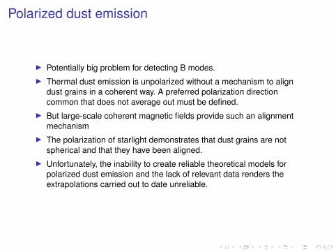
Polarized dust emission

I Potentially big problem for detecting B modes.I Thermal dust emission is unpolarized without a mechanism to align

dust grains in a coherent way. A preferred polarization directioncommon that does not average out must be defined.

I But large-scale coherent magnetic fields provide such an alignmentmechanism

I The polarization of starlight demonstrates that dust grains are notspherical and that they have been aligned.

I Unfortunately, the inability to create reliable theoretical models forpolarized dust emission and the lack of relevant data renders theextrapolations carried out to date unreliable.

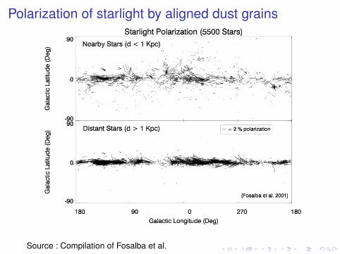
Polarization of starlight by aligned dust grains

Source : Compilation of Fosalba et al.

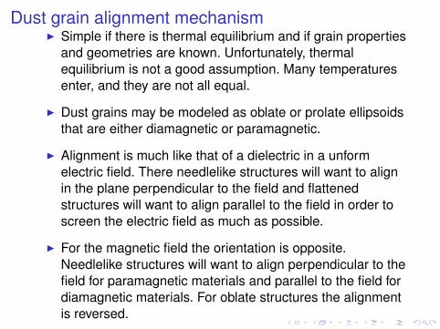
Dust grain alignment mechanismI Simple if there is thermal equilibrium and if grain properties

and geometries are known. Unfortunately, thermalequilibrium is not a good assumption. Many temperaturesenter, and they are not all equal.

I Dust grains may be modeled as oblate or prolate ellipsoidsthat are either diamagnetic or paramagnetic.

I Alignment is much like that of a dielectric in a unformelectric field. There needlelike structures will want to alignin the plane perpendicular to the field and flattenedstructures will want to align parallel to the field in order toscreen the electric field as much as possible.

I For the magnetic field the orientation is opposite.Needlelike structures will want to align perpendicular to thefield for paramagnetic materials and parallel to the field fordiamagnetic materials. For oblate structures the alignmentis reversed.

I Typical dimensionless susceptibilities are of order 1e-5.Thermodynamic considerations will limit the degree ofalignment.

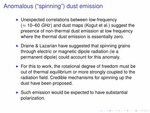
Anomalous (“spinning”) dust emission

I Unexpected correlations between low-frequency(≈ 10–60 GHz) and dust maps (Kogut et al.) suggest thepresence of non-thermal dust emission at low frequencywhere the thermal dust emission is essentially zero.

I Draine & Lazarian have suggested that spinning grainsthrough electric or magnetic dipole radiation (ie apermanent dipole) could account for this anomaly.

I For this to work, the rotational degree of freedom must beout of thermal equilibrium or more strongly coupled to theradiation field. Credible mechanisms for spinning up thedust have been proposed.

I Such emission would be expected to have substantialpolarization.

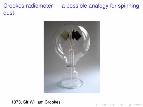
Crookes radiometer — a possible analogy for spinningdust

1873, Sir William Crookes

Rotational properties of dust grains

I For the non-rotational degrees of freedom of dust grains, there is a balancebetween UV flux from stars that is absorbed and the subsequent re-emission atinfrared and microwave frequencies. For small grains, incident photons arriveinfrequently, maybe one a day, raising their temperature to mayeb 150 K, andthen they decay maybe in 100 sec to a very low temperature slightly above theCMB temperature. These are the grains responsible for the small-wavelengthpart of the dust emission spectrum. Larger grains, on the other hand, receivephotons frequently and maintain a nearly constant temperature, around 17 K.There emission is restricted to long wavelengths by the exponential factor in theBoltzmann distribution.

I The rotational degrees of freedom, however, are special. A number of effectscouple only to the rigid degrees of freedom and not to the other internal degreesof freedom, and can spin up a dust grain. There are also emission mechanismsthat are couple only to the rotational mode. For this reason it does make sense tothink about “Suprathermal rotational of interstellar dust grains” (a paper title ofEM Purcell in 1979 on the subject).

I Collisions with molecules would tend to spin up the rotational degree of freedomso that its energy is given by the ambient kinetic gas temperature, in thethousands of degrees.

Rotational properties of dust grains (II)

I Catalysis of the formation of molecular hydrogen on the dust grain, perhaps at aparticular non-random site releases 4.2eV, a huge amount of recoil applying atorque to the rotational degree of freedom, likely in a coherent way. This is morelike an engine extracting energy from an out-of-equilibrium situation.

I Non-uniform radiation pressure will also exert a torque. In general the absorptionproperties across the grain will be non-uniform, causing the incident radiation toexert a torque in a coherent. Again, thermodynamically this is much like anengine. The hot temperature is the UV radiation expelled as at a lowertemperature (the thermal IR radiation). The net torque would vanish if the twotemperatures were equal.

I Dust grains in general have a permanent electric dipole moment, and likenon-symmetric diatomic molecules (eg CO). If they are charged, their center ofcharge is unlikely to coincide precisely with their center of mass. This means thatrotating dust grains act as dipole radiators, with the radiated power proportionalto the fourth power of the angular velocity. This provides a mechanism to limit theangular velocity of a grain.

I This is all very complicated. The necessary information for reliable modelling islacking. (Papers by Draine, Lazarian, and especially older papers by Purcell offeran invaluable source of information.)

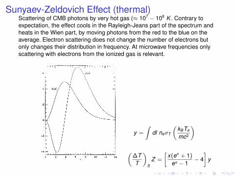
Sunyaev-Zeldovich Effect (thermal)Scattering of CMB photons by very hot gas (≈ 107 − 108 K . Contrary toexpectation, the effect cools in the Rayleigh-Jeans part of the spectrum andheats in the Wien part, by moving photons from the red to the blue on theaverage. Electron scattering does not change the number of electrons butonly changes their distribution in frequency. At microwave frequencies onlyscattering with electrons from the ionized gas is relevant.

y =

Zdl neσT

„kBTe

mc2

«„

∆TT

«S

Z =

»x(ex + 1)

ex − 1− 4–

y

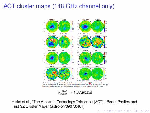
ACT cluster maps (148 GHz channel only)

σFWMHbeam ≈ 1.37arcmin

Hinks et al., “The Atacama Cosmology Telescope (ACT) : Beam Profiles andFirst SZ Cluster Maps” (astro-ph/0907.0461)

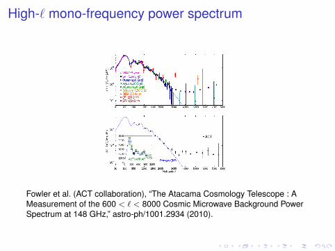
High-` mono-frequency power spectrum

Fowler et al. (ACT collaboration), “The Atacama Cosmology Telescope : AMeasurement of the 600 < ` < 8000 Cosmic Microwave Background PowerSpectrum at 148 GHz,” astro-ph/1001.2934 (2010).

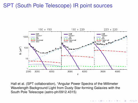
SPT (South Pole Telescope) IR point sources

Hall et al. (SPT collaboration), “Angular Power Spectra of the MillimeterWavelength Background Light from Dusty Star-forming Galaxies with theSouth Pole Telescope (astro-ph/0912.4315)

Kinetic Sunyaev-Zeldovich & Ostriker-Vishniac effect(much smaller than the thermal SZ effect and easily confused withcosmological perturbations because of its blackbody spectral form)

„∆TT

«Ostriker−Vishniac

(bΩ) =

Z η0

0dηa(η)ne(η)σT exp[−τ ]

hbΩ · v(bΩ(η0 − η), η)i

=

Z ∞0

dτσT exp[−τ ]hbΩ · v(bΩ(η0 − η(tau)), η)

i„

∆TT

«kSZ

= τcluster

“vpec

c

”Three related effects are incorporated within a single formula :

I (1) kinetic Sunyaev-Zeldovich (fully collapsed and virialized objects)I (2) Ostriker-Vishniac (in the field, higher-order perturbation theory, later

times,I (3) patchy reionization (emphasizes the effect of sharp edges of the

electron density, due to Strömgen spheres....).

These should be though of as aspect of a single effect because thedistinctions between them cannot be cleanly differentiated.

Point sources

I Two basic types : radio point sources [arising from synchrotronemission in compact objects (e.g., radio-loud AGNs, "flat spectrum"radion galaxies, BL-Lacs,....), and IR points sources (dusty galaxieswith hot thermal dust emission)

I Point sources dominate at high-`. May be approximated as aPoissonian distribution of pointlike objects on the celestial sphere. Butthese two simplifying approximations have their limitations, especiallyas increasingly smaller scales are being probed. Clustering complicatesconstructing a template to account for unsubtracted point sources.

I Unfortunately, their spectral indices vary considerably ; therefore, toidentify either in high frequency or low frequency maps and mask in theintermediate "CMB" frequencies is a good strategy for the mostluminous objects. Nevertheless, a background of unresolved pointsources is predicted to subsist.

Foreground removal techniques

There is no silver bullet for this problem. There are many approaches andsince the problem is hard and no unambiguous solution suggests itself, onewant to try every reasonable approach and compare results.

Approaches can be based on :I (1) Understanding and modelling the detailed physics of the foreground

components and other contaminants.I (2) Data analysis. Study of correlations. Template subtraction.I (3) Blind analyses (e.g. independent component analysis, internal linear

combination). Best for looking for unexpected new components in thedata.

I (4) Bayesian modelling. Expressing what is known as best as possiblein terms of priors which compete with eacg other and are rationallyresolved in accordance with Bayes theorem.

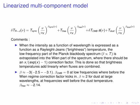
Linearized multi-component model

δTR−J (ν) = Tsync

„ν

νK

«βsync (ν)

+Tfree

„ν

νK

«βfree(ν)

+δTCMB a(ν)+Tdust

„ν

νK

«βdust (ν)

Comments :I When the intensity as a function of wavelength is expressed as a

function as a Rayleight-Jeans (“brightness”) temperature, thelow-frequency part of the Planck blackbody spectrum (I ∝ T ) isextrapolated into the Wien part of the spectrum, where there should bean x/(exp(x)− 1) correction factor. This is done so that brightnesstemperatures add linearly when fluxes are combined.

I β ≈ −3(−2.5 – −3.1). βCMB = 0 at low frequencies where before theWien regime correction factor kicks in. β ≈ 2 for dust at largewavelengths, at frequencies well before the dust temperature.βfree ≈ −2.14.

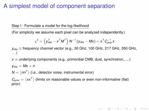
A simplest model of component separation

Step I : Formulate a model for the log-likelihood

(For simplicity we assume each pixel can be analyzed independently.)

χ2 =“

yTobs − xT MT

”N−1 (yobs −Mx) + xT C−1

prior x

yobs ≡ frequency channel vector (e.g., 30 Ghz, 100 GHz, 217 GHz, 350 GHz,. . .)

x ≡ underlying components (e.g., primordial CMB, dust, synchrotron,.....)

yobs = Mx + n

N =˙nnT ¸ (i.e., detector noise, instrumental error)

Cprior =˙xxT ¸ (limits on reasonable values or even non-informative (flat)

prior)

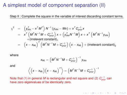
A simplest model of component separation (II)

Step II : Complete the square in the variable of interest discarding constant terms.

χ2 =“

yTobs − xT MT

”N−1 (yobs −Mx) + xT C−1

prior x

= xT“

MT N−1M + C−1prior

”x +

“yT

obsN−1M”

x + xT“

MT N−1yobs

”+(irrelevant constant)1

=“

x − xML

”T “MT N−1M + C−1

prior

”“x − xML

”+ (irrelevant constant)2

wherexML =

“MT N−1M + C−1

prior

”−1yobs

and fi“x − xML

”“x − xML

”Tfl

=“

MT N−1M + C−1prior

”−1

Note that (1) in general M is rectangular and not square and (2) C−1prior can

have zero eigenvalues of be identically zero.

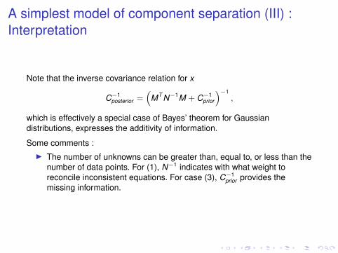
A simplest model of component separation (III) :Interpretation

Note that the inverse covariance relation for x

C−1posterior =

“MT N−1M + C−1

prior

”−1,

which is effectively a special case of Bayes’ theorem for Gaussiandistributions, expresses the additivity of information.

Some comments :I The number of unknowns can be greater than, equal to, or less than the

number of data points. For (1), N−1 indicates with what weight toreconcile inconsistent equations. For case (3), C−1

prior provides themissing information.

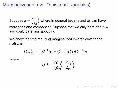
Marginalization (over “nuisance” variables)

Suppose x =

(x1x2

)where in general both x1 and x2 can have

more than one component. Suppose that we only care about x1and could care less about x2.

We show that the resulting marginalized inverse covariancematrix is

(C−1marg) = (C−1)11 − (C−1)12C22(C−1)21

where

C−1 =

(C−1

11 C−112

C−121 C−1

22

).

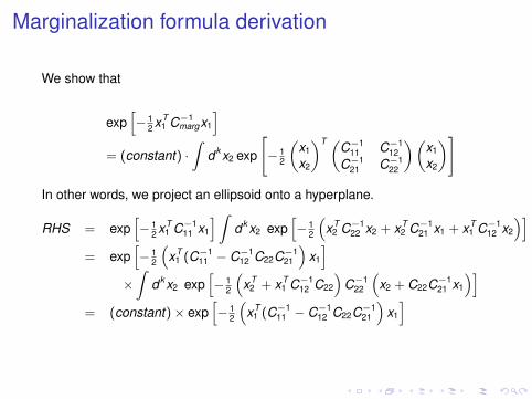
Marginalization formula derivation

We show that

exph− 1

2 xT1 C−1

margx1

i= (constant) ·

Zdk x2 exp

"− 1

2

„x1

x2

«T „C−111 C−1

12C−1

21 C−122

«„x1

x2

«#

In other words, we project an ellipsoid onto a hyperplane.

RHS = exph− 1

2 xT1 C−1

11 x1

i Zdk x2 exp

h− 1

2

“xT

2 C−122 x2 + xT

2 C−121 x1 + xT

1 C−112 x2

”i= exp

h− 1

2

“xT

1 (C−111 − C−1

12 C22C−121

”x1

i×Z

dk x2 exph− 1

2

“xT

2 + xT1 C−1

12 C22

”C−1

22

“x2 + C22C−1

21 x1

”i= (constant)× exp

h− 1

2

“xT

1 (C−111 − C−1

12 C22C−121

”x1

i

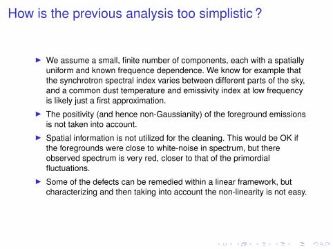
How is the previous analysis too simplistic ?

I We assume a small, finite number of components, each with a spatiallyuniform and known frequence dependence. We know for example thatthe synchrotron spectral index varies between different parts of the sky,and a common dust temperature and emissivity index at low frequencyis likely just a first approximation.

I The positivity (and hence non-Gaussianity) of the foreground emissionsis not taken into account.

I Spatial information is not utilized for the cleaning. This would be OK ifthe foregrounds were close to white-noise in spectrum, but thereobserved spectrum is very red, closer to that of the primordialfluctuations.

I Some of the defects can be remedied within a linear framework, butcharacterizing and then taking into account the non-linearity is not easy.

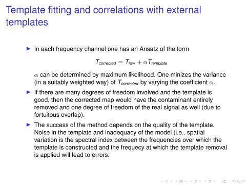
Template fitting and correlations with externaltemplates

I In each frequency channel one has an Ansatz of the form

Tcorrected = Traw + αTtemplate

α can be determined by maximum likelihood. One minizes the variance(in a suitably weighted way) of Tcorrected by varying the coefficient α.

I If there are many degrees of freedom involved and the template isgood, then the corrected map would have the contaminant entirelyremoved and one degree of freedom of the real signal as well (due tofortuitous overlap).

I The success of the method depends on the quality of the template.Noise in the template and inadequacy of the model (i.e., spatialvariation is the spectral index between the frequencies over which thetemplate is constructed and the frequecy at which the template removalis applied will lead to errors.

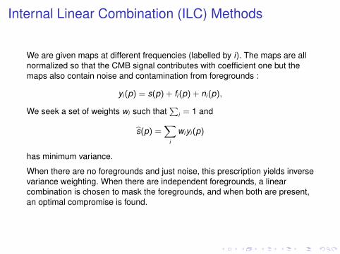
Internal Linear Combination (ILC) Methods

We are given maps at different frequencies (labelled by i). The maps are allnormalized so that the CMB signal contributes with coefficient one but themaps also contain noise and contamination from foregrounds :

yi (p) = s(p) + fi (p) + ni (p),

We seek a set of weights wi such thatP

i = 1 and

bs(p) =X

i

wiyi (p)

has minimum variance.

When there are no foregrounds and just noise, this prescription yields inversevariance weighting. When there are independent foregrounds, a linearcombination is chosen to mask the foregrounds, and when both are present,an optimal compromise is found.

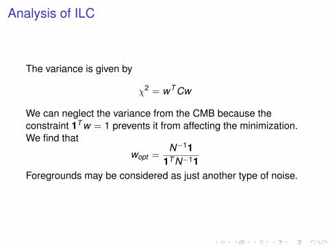
Analysis of ILC

The variance is given by

χ2 = wT Cw

We can neglect the variance from the CMB because theconstraint 1T w = 1 prevents it from affecting the minimization.We find that

wopt =N−11

1T N−11Foregrounds may be considered as just another type of noise.

Weaknesses of the ILC

I Given that the statistical properties of the foregrounds are not uniformover the sky, the variance of the overall ILC map as a figure of merit isnot appropriate. This prescription favors linear combinations that workwell in the galactic plane where the foregrounds are largest, but thelinear combination obtained is likely not to be obtained in the low-noiseregions of the map, which carry the most information. The fineness ofthe pixelization also enters into determining the optimal combination.One may want to use different linear combinations in different regions ofharmonic space. Prior information is not exploited.

I In practice these problems have been alleviated by separating the skyinto several zones suitably matched, with ILC applied independently tothe several regions.

Independent component analysis (ICA)I This ‘blind’ method seeks to extract a number of components from the

data without any prior information.I Let x be the component vector and d the data vector. One seekis a

mixing matrix M and a component vector x such that

χ2 = (d −Mx)T N−1(d −Mx)

is minimized where d is the data vector. One seeks that the componentsbe “independent” or orthogonal in an appropriately defined way.

I One of the problems is that is all the distributions are supposed to beGaussian, the distinction between the components disppears. Apartfrom multiplicative (rescalings of the components), one can mix thecomponents among themselves using an orthogonal matrix O, so thatx → 0x , and M → MOT while maintaining their independence.

I Several solutions have been proposed to this problem, one of which isto maximize the degree of non-Gaussianity of the components. By thecentral limit theorem, mixtures of the non-Gaussian components (whatone seeks to avoid) increases the Gaussianity.

I In practice ICA-based methods work quite well, despite their lack of arigorous foundation.

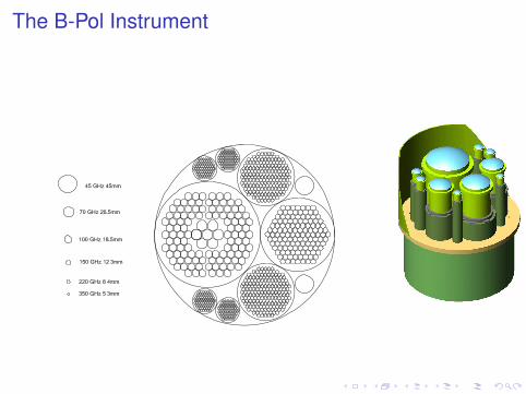
The B-Pol Instrument

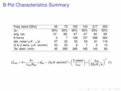
B-Pol Characteristics Summary

Freq. band (GHz) 45 70 100 143 217 353∆ν 30% 30% 30% 30% 30% 30%ang. res. 15 68’ 47’ 47’ 40’ 59’# horns 2 7 108 127 398 364det. noise (µK ·

√s) 57 33 53 53 61 119

Q & U sens. (µK · arcmin) 33 23 8 7 5 10Tel. diam. (mm) 45 265 265 185 143 60

c2noise = 4× 4π

tmissNdet×s2

det = (5µK ·arcmin)2ׄ

2 yearstmiss

«×„

sdet

50µK√

s

«2

(1)