Lecture29 AT620 110711 - Colorado State...
32
Virtual temperature • AMS glossary: (h/p://amsglossary.allenpress.com/glossary/search?id=virtualtemperature1 ) • virtual temperature—(Also called density temperature.) The virtual temperature is computed from T v = T(1 + r v / ε)/(1 + r v ), where r v is the mixing raIo of water vapor and ε is the raIo of the gas constants of air and water vapor , ≈ 0.622. • Always warmer than the physical temperature (corresponds to decrease in density due to water vapor; biggest deviaIons in moist boundary layer). – The virtual temperature allows the use of the dryair equaIon of state for moist air , except with T replaced by T v . – The virtual temperature is the temperature that dry dry air would have if its pressure and density were equal to those of a given sample of moist air. – For typical observed values of r v , the virtual temperature may be approximated by T v = (1 + 0.61 r v ) T. – Some authors incorporate the density increment due to liquid or solid water into virtual temperature, in which case the definiIon becomes T v = T(1 + r v /ε)/ (1 + r v + r l )≈ T(1 + 0.61r v − r l ), where r l is the liquid or liquid plus solid water mixing raIo.
-
Upload
vuongquynh -
Category
Documents
-
view
229 -
download
0
Transcript of Lecture29 AT620 110711 - Colorado State...
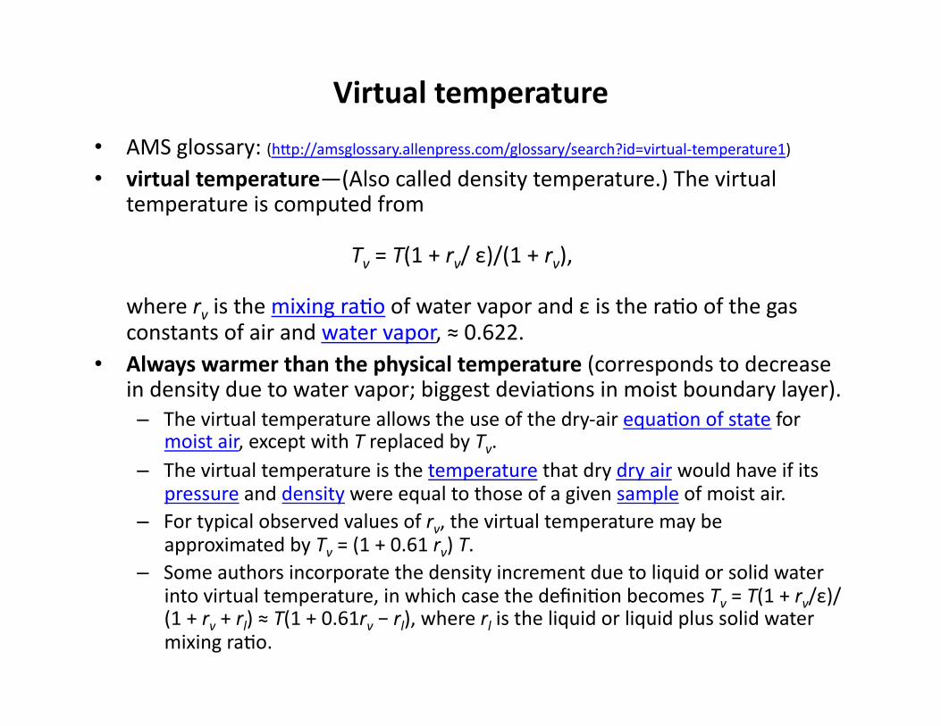
Virtual temperature
• AMS glossary: (h/p://amsglossary.allenpress.com/glossary/search?id=virtual-‐temperature1)
• virtual temperature—(Also called density temperature.) The virtual temperature is computed from
Tv = T(1 + rv/ ε)/(1 + rv),
where rv is the mixing raIo of water vapor and ε is the raIo of the gas constants of air and water vapor, ≈ 0.622.
• Always warmer than the physical temperature (corresponds to decrease in density due to water vapor; biggest deviaIons in moist boundary layer). – The virtual temperature allows the use of the dry-‐air equaIon of state for
moist air, except with T replaced by Tv. – The virtual temperature is the temperature that dry dry air would have if its
pressure and density were equal to those of a given sample of moist air. – For typical observed values of rv, the virtual temperature may be
approximated by Tv = (1 + 0.61 rv) T. – Some authors incorporate the density increment due to liquid or solid water
into virtual temperature, in which case the definiIon becomes Tv = T(1 + rv/ε)/(1 + rv + rl) ≈ T(1 + 0.61rv − rl), where rl is the liquid or liquid plus solid water mixing raIo.
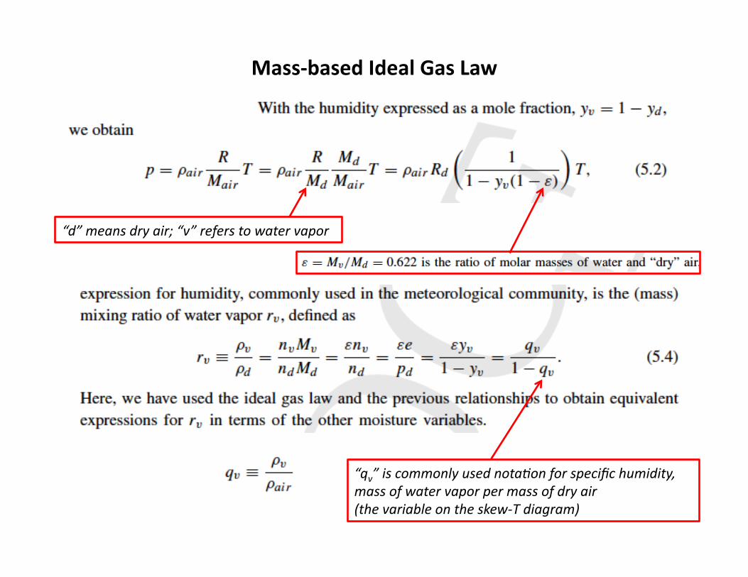
Mass-‐based Ideal Gas Law
“d” means dry air; “v” refers to water vapor
“qv” is commonly used nota9on for specific humidity, mass of water vapor per mass of dry air (the variable on the skew-‐T diagram)
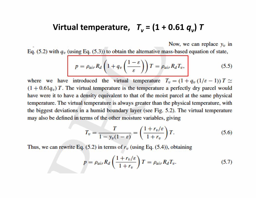
Virtual temperature, Tv = (1 + 0.61 qv) T
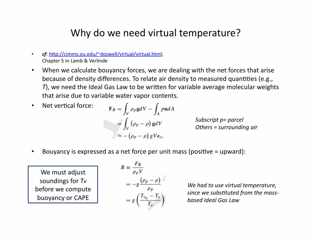
Why do we need virtual temperature?
• cf: h/p://cimms.ou.edu/~doswell/virtual/virtual.html; Chapter 5 in Lamb & Verlinde
• When we calculate bouyancy forces, we are dealing with the net forces that arise because of density differences. To relate air density to measured quanIIes (e.g., T), we need the Ideal Gas Law to be wri/en for variable average molecular weights that arise due to variable water vapor contents.
• Net verIcal force:
• Bouyancy is expressed as a net force per unit mass (posiIve = upward):
Subscript p= parcel Others = surrounding air
We had to use virtual temperature, since we subs9tuted from the mass-‐based Ideal Gas Law
We must adjust soundings for Tv
before we compute buoyancy or CAPE
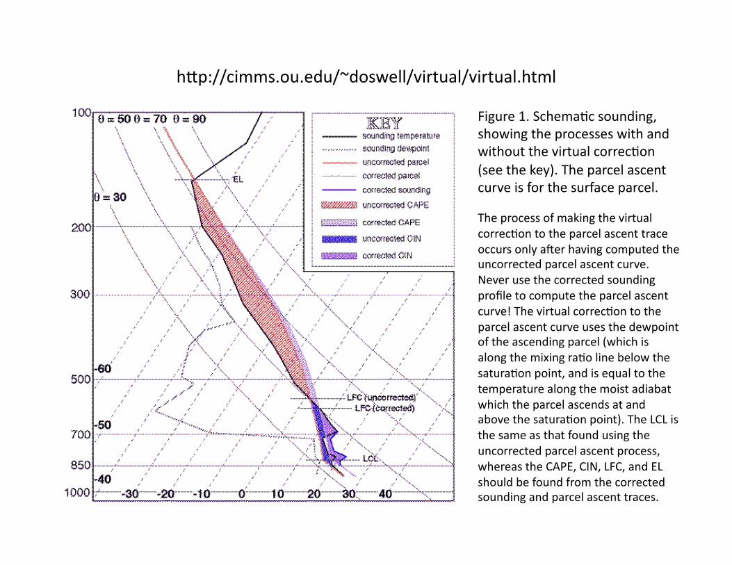
h/p://cimms.ou.edu/~doswell/virtual/virtual.html
Figure 1. SchemaIc sounding, showing the processes with and without the virtual correcIon (see the key). The parcel ascent curve is for the surface parcel.
The process of making the virtual correcIon to the parcel ascent trace occurs only ader having computed the uncorrected parcel ascent curve. Never use the corrected sounding profile to compute the parcel ascent curve! The virtual correcIon to the parcel ascent curve uses the dewpoint of the ascending parcel (which is along the mixing raIo line below the saturaIon point, and is equal to the temperature along the moist adiabat which the parcel ascends at and above the saturaIon point). The LCL is the same as that found using the uncorrected parcel ascent process, whereas the CAPE, CIN, LFC, and EL should be found from the corrected sounding and parcel ascent traces.
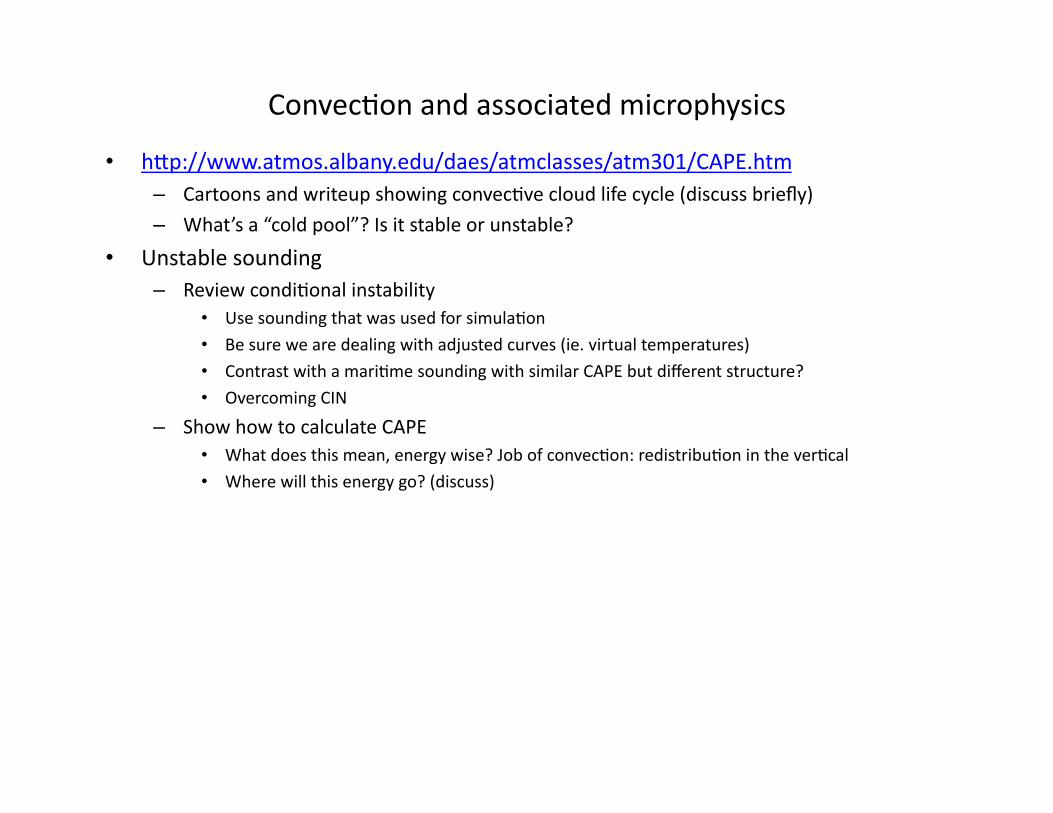
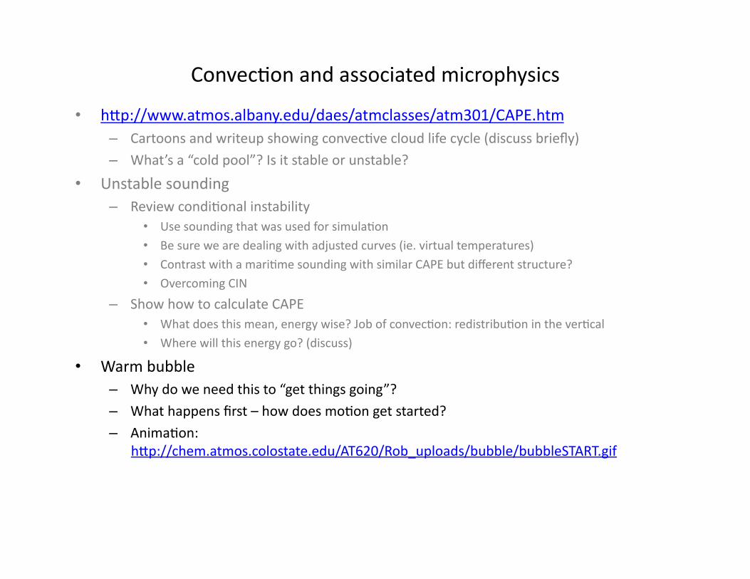
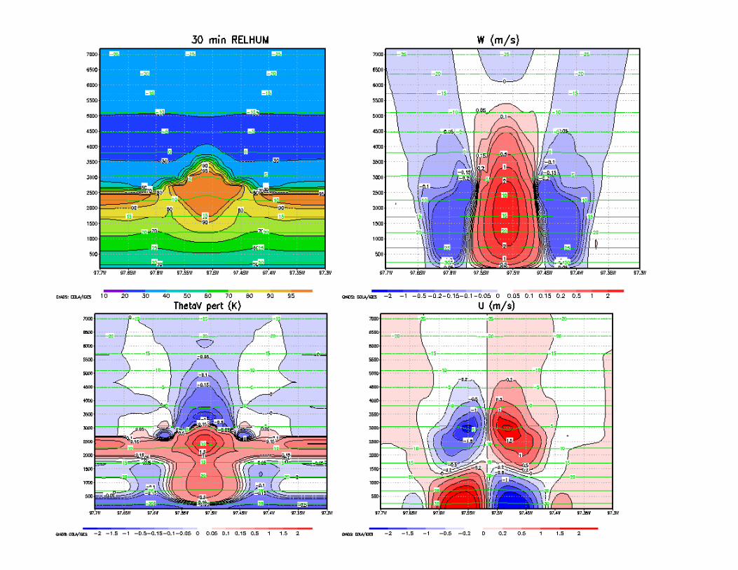
ConvecIon and associated microphysics
• h/p://www.atmos.albany.edu/daes/atmclasses/atm301/CAPE.htm – Cartoons and writeup showing convecIve cloud life cycle (discuss briefly)
– What’s a “cold pool”? Is it stable or unstable?
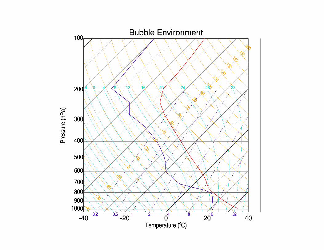
• Unstable sounding – Review condiIonal instability
• Use sounding that was used for simulaIon • Be sure we are dealing with adjusted curves (ie. virtual temperatures) • Contrast with a mariIme sounding with similar CAPE but different structure? • Overcoming CIN
– Show how to calculate CAPE • What does this mean, energy wise? Job of convecIon: redistribuIon in the verIcal • Where will this energy go? (discuss)
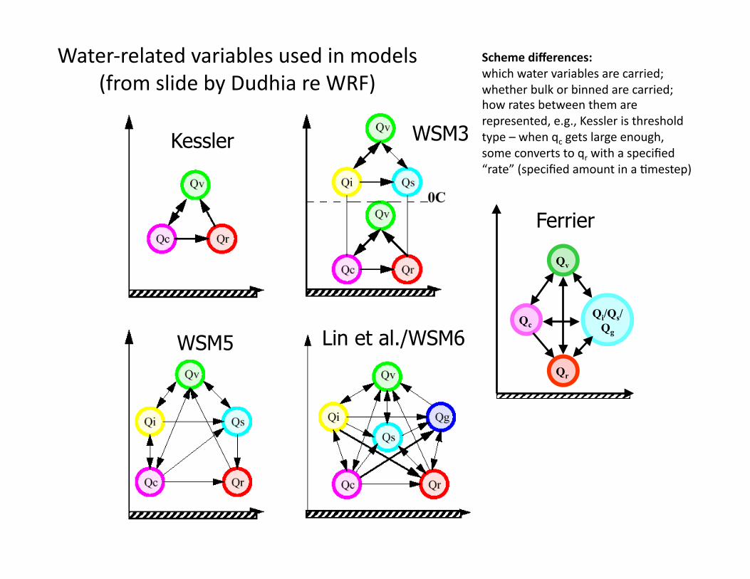
Water-‐related variables used in models (from slide by Dudhia re WRF)
Ferrier
Qi/Qs/ Qg
Qv
Qc
Qr
Kessler WSM3
Lin et al./WSM6 WSM5
Illustration of Microphysics Processes
Scheme differences: which water variables are carried; whether bulk or binned are carried; how rates between them are represented, e.g., Kessler is threshold type – when qc gets large enough, some converts to qr with a specified “rate” (specified amount in a Imestep)
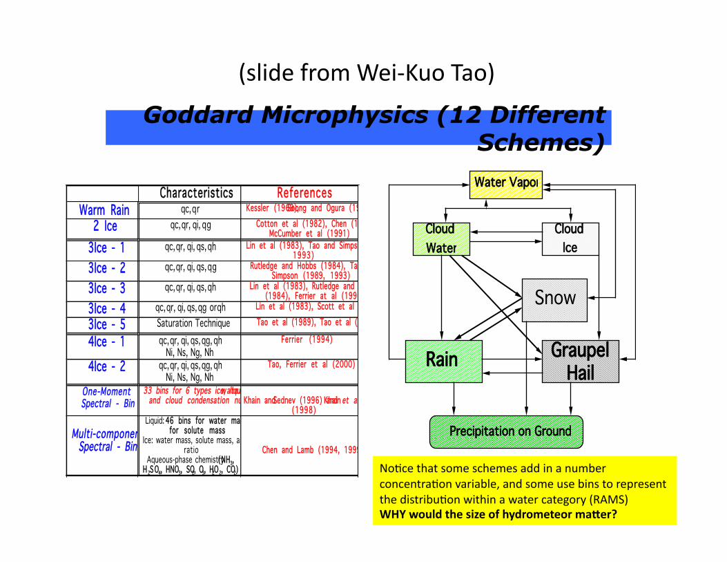
(slide from Wei-‐Kuo Tao)
Goddard Microphysics (12 DifferentSchemes)
Cloud
Water
Water Vapor
Rain GraupelHail
Precipitation on Ground
Snow
Cloud
Ice
Characteristics ReferencesWarm Rain qc, qr Kessler (1969), Soong and Ogura (1973)
2 Ice qc, qr, qi, qg Cotton et al (1982), Chen (1983),McCumber et al (1991)
3Ice - 1 qc, qr, qi, qs, qh Lin et al (1983), Tao and Simpson (1989,1993)
3Ice - 2 qc, qr, qi, qs, qg Rutledge and Hobbs (1984), Tao andSimpson (1989, 1993)
3Ice - 3 qc, qr, qi, qs, qh Lin et al (1983), Rutledge and Hobbs(1984), Ferrier at al (1995)
3Ice - 4 qc, qr, qi, qs, qg or qh Lin et al (1983), Scott et al (2000)
3Ice - 5 Saturation Technique Tao et al (1989), Tao et al (2000)
4Ice - 1 qc, qr, qi, qs, qg, qhNi, Ns, Ng, Nh
Ferrier (1994)
4Ice - 2 qc, qr, qi, qs, qg, qhNi, Ns, Ng, Nh
Tao, Ferrier et al (2000)
One-MomentSpectral - Bin
33 bins for 6 types ice, liquid wate rand cloud condensation nucleiKhain and Sednev (1996) and Khain et al.
(1998)
Multi-componentSpectral - Bin
Liquid: 46 bins for water mass, 25for solute mass
Ice: water mass, solute mass, aspectratio
Aqueous-phase chemistry (NH3,H 2SO4, HNO3, SO2, O3, H2O2, CO2)
Chen and Lamb (1994, 1999)
No Microphysical Scheme is perfect !
NoIce that some schemes add in a number concentraIon variable, and some use bins to represent the distribuIon within a water category (RAMS) WHY would the size of hydrometeor maMer?
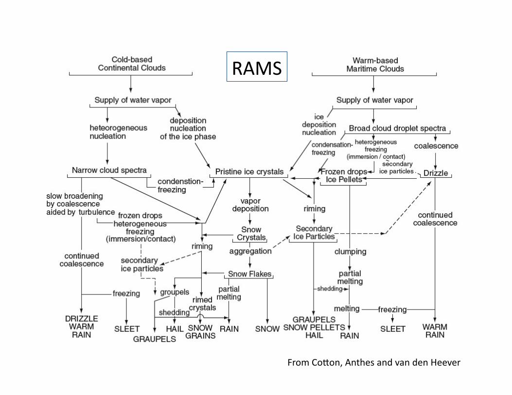
From Co/on, Anthes and van den Heever
RAMS
ConvecIon and associated microphysics
• h/p://www.atmos.albany.edu/daes/atmclasses/atm301/CAPE.htm – Cartoons and writeup showing convecIve cloud life cycle (discuss briefly)
– What’s a “cold pool”? Is it stable or unstable?
• Unstable sounding – Review condiIonal instability
• Use sounding that was used for simulaIon • Be sure we are dealing with adjusted curves (ie. virtual temperatures) • Contrast with a mariIme sounding with similar CAPE but different structure? • Overcoming CIN
– Show how to calculate CAPE • What does this mean, energy wise? Job of convecIon: redistribuIon in the verIcal • Where will this energy go? (discuss)
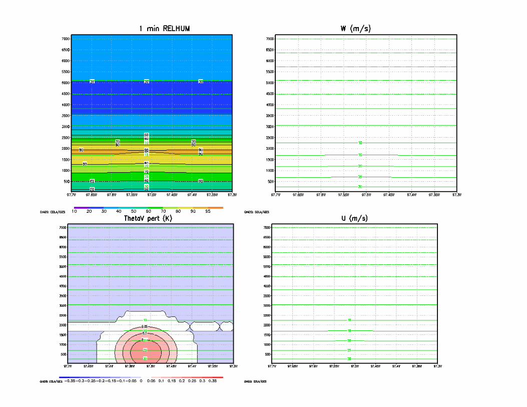
• Warm bubble – Why do we need this to “get things going”?
– What happens first – how does moIon get started?
– AnimaIon: h/p://chem.atmos.colostate.edu/AT620/Rob_uploads/bubble/bubbleSTART.gif
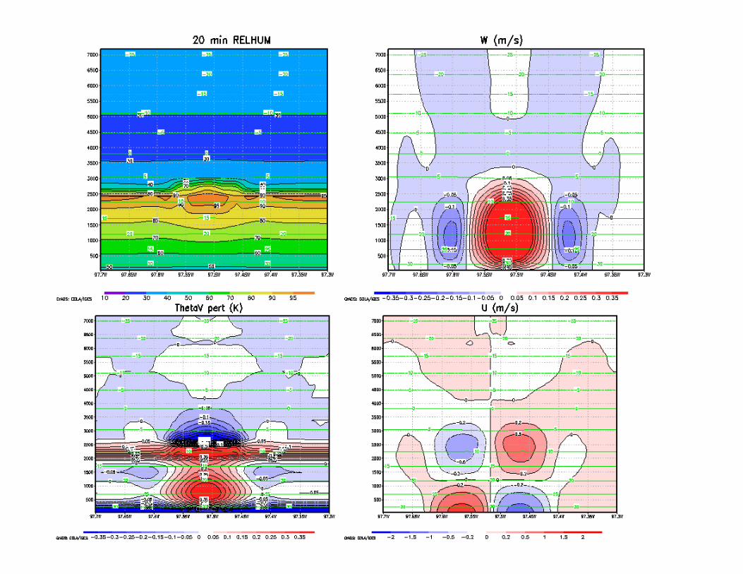
ConvecIon and associated microphysics
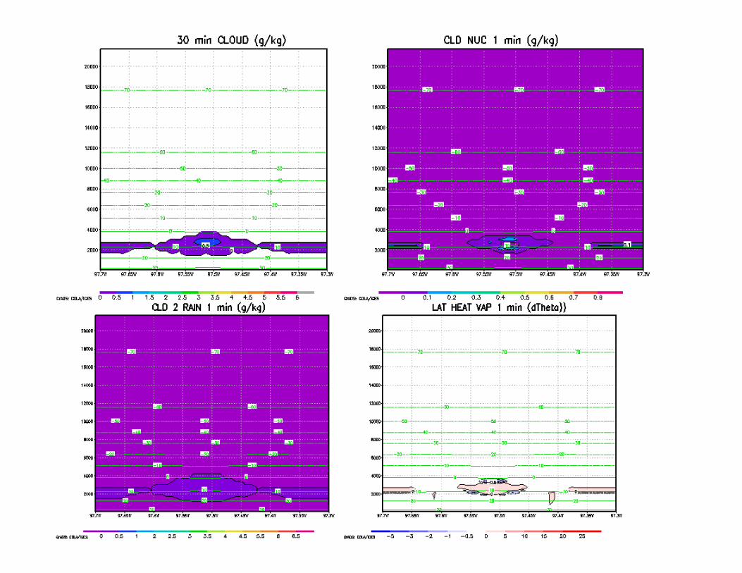
• How are microphysical processes evolving? – When do we start to see cloud water converIng into rain?
– Where in the cloud is this occurring?
– What are the associated heat releases?
– AnimaIon: h/p://chem.atmos.colostate.edu/AT620/Rob_uploads/bubble/bubbleCLD.gif
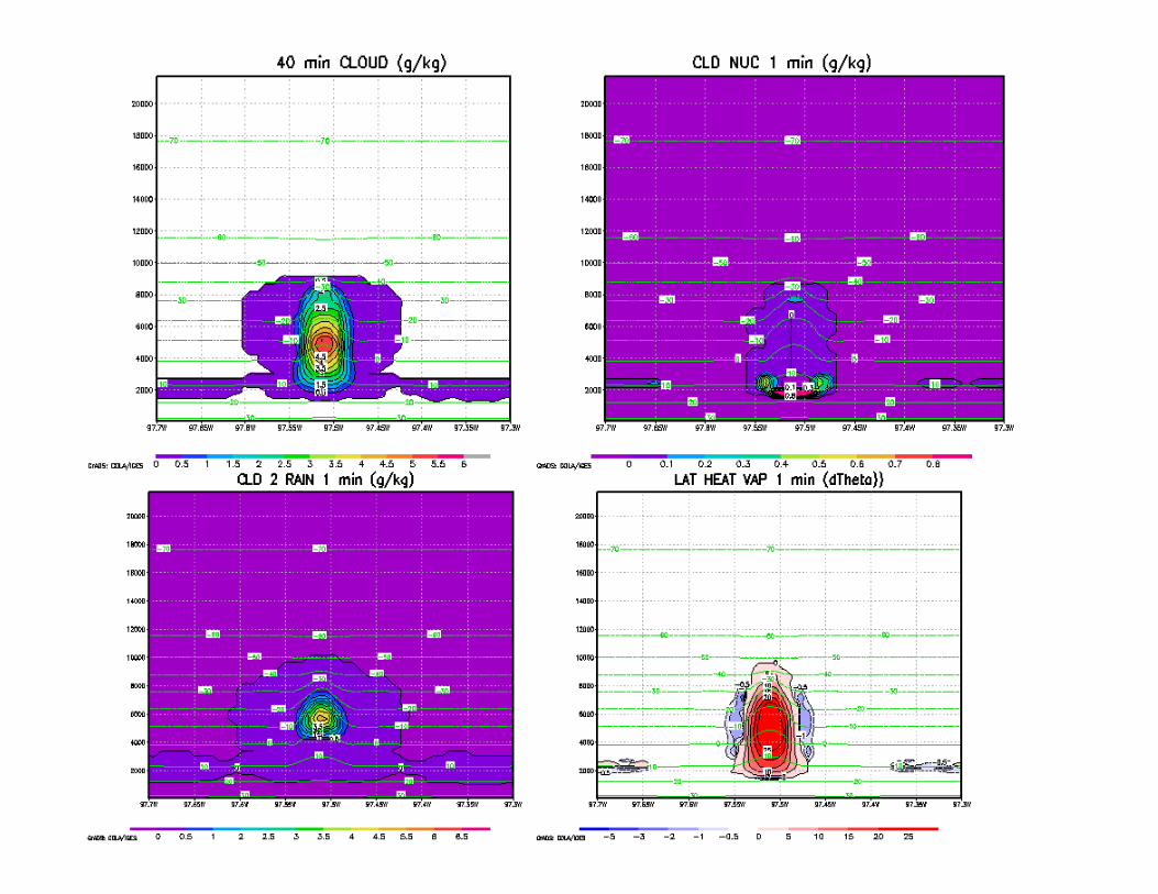

Sketch sounding at 40 min
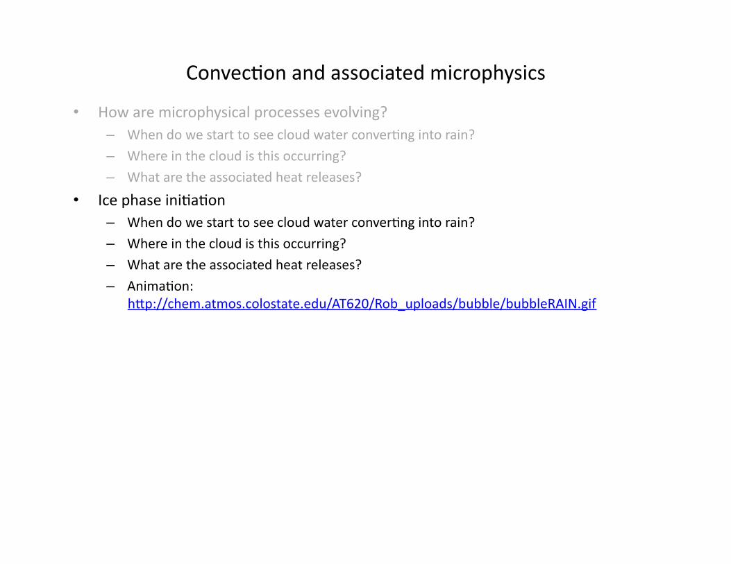
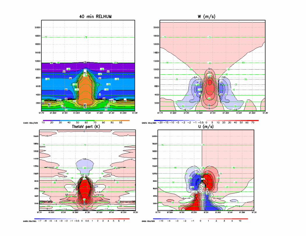
ConvecIon and associated microphysics
• How are microphysical processes evolving? – When do we start to see cloud water converIng into rain?
– Where in the cloud is this occurring?
– What are the associated heat releases?
• Ice phase iniIaIon – When do we start to see cloud water converIng into rain?
– Where in the cloud is this occurring?
– What are the associated heat releases?
– AnimaIon: h/p://chem.atmos.colostate.edu/AT620/Rob_uploads/bubble/bubbleRAIN.gif
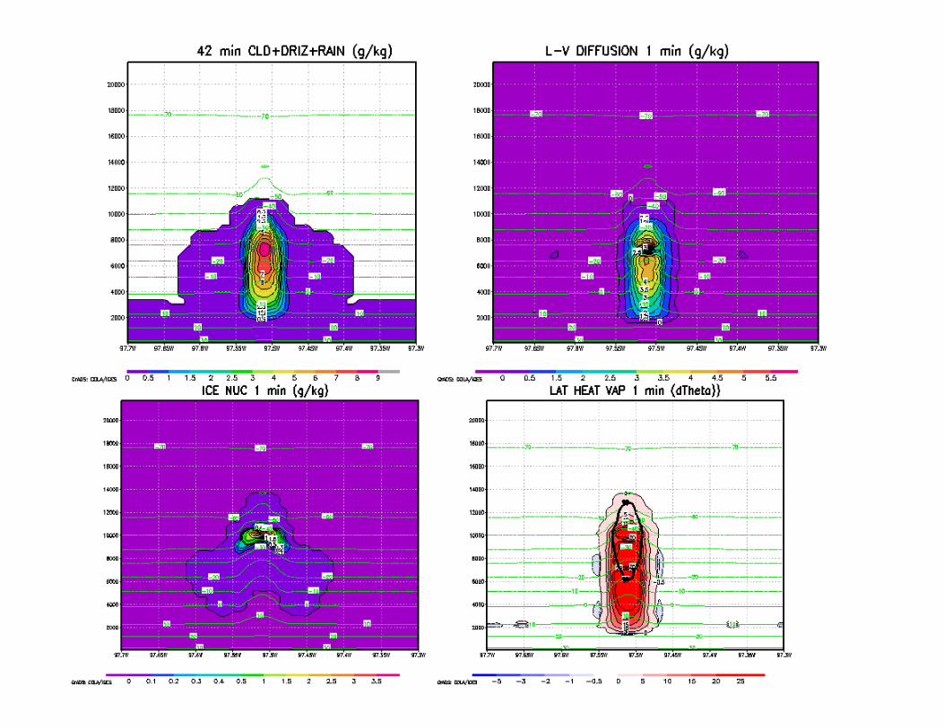
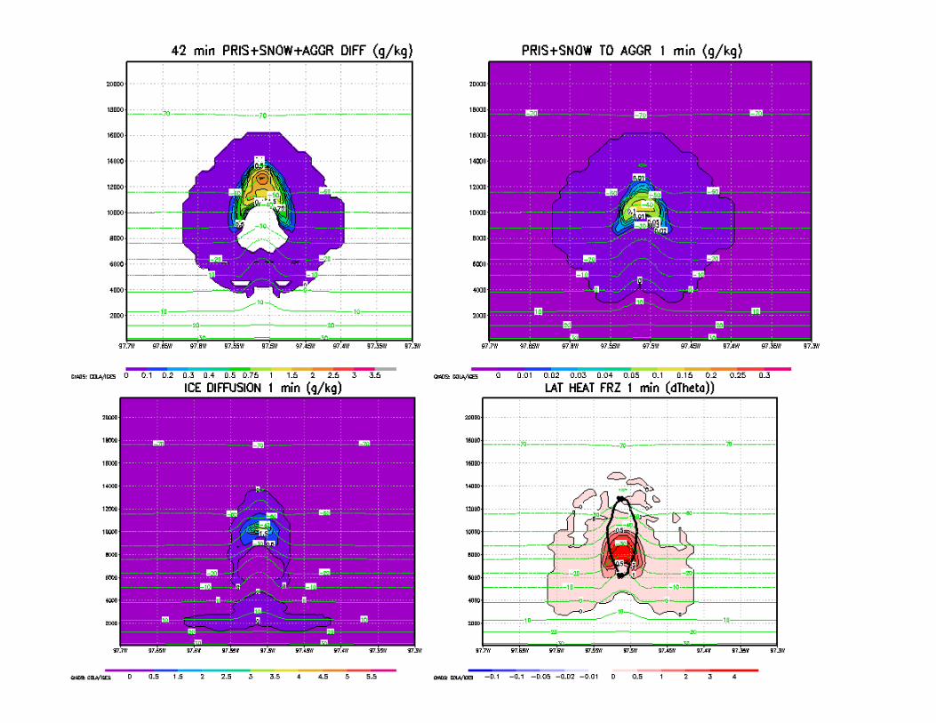
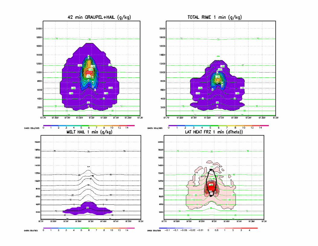
• Ice species evoluIon – What are the rates at which water is being transferred into other species?
– Where in the cloud does this occur?
– AnimaIon: h/p://chem.atmos.colostate.edu/AT620/Rob_uploads/bubble/bubbleICE.gif
– AnimaIon: h/p://chem.atmos.colostate.edu/AT620/Rob_uploads/bubble/bubbleHAIL.gif
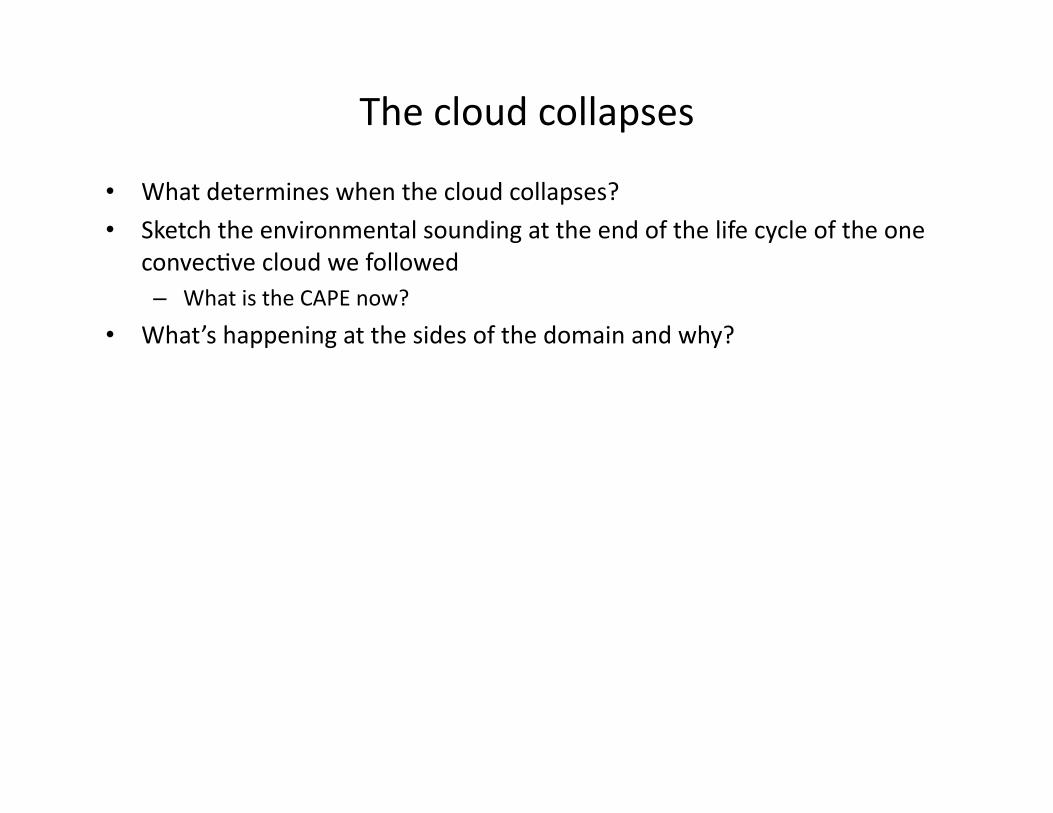
The cloud collapses
• What determines when the cloud collapses?
• Sketch the environmental sounding at the end of the life cycle of the one convecIve cloud we followed – What is the CAPE now?
• What’s happening at the sides of the domain and why?
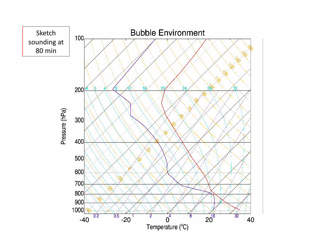
Sketch sounding at 80 min

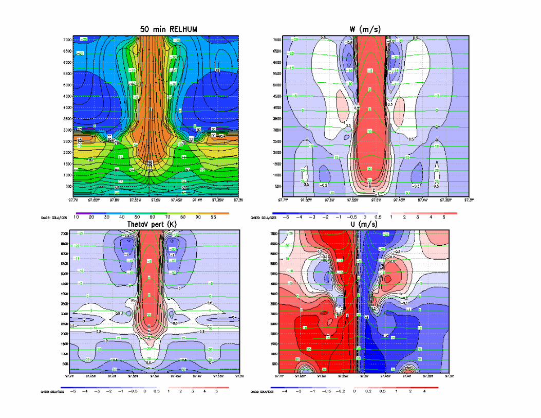
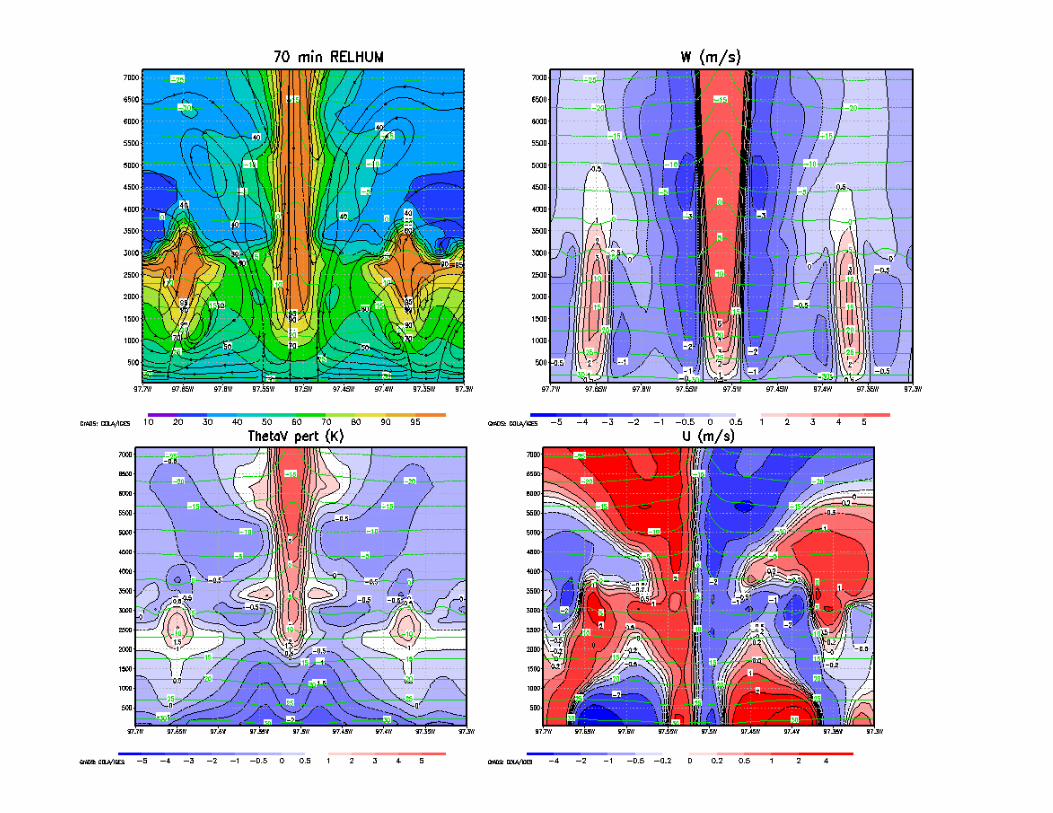
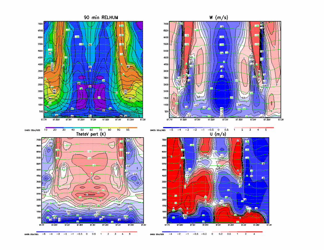
The cold pool
• What iniIated the cold pool?
• Where does the cold pool first form? Why?
• What role does the cold pool play in subsequent convecIon?
• When does the cold pool become ‘strongest’? How can we define cold pool ‘strength’?
• AnimaIon: h/p://chem.atmos.colostate.edu/AT620/Rob_uploads/bubble/bubbleCP.gif
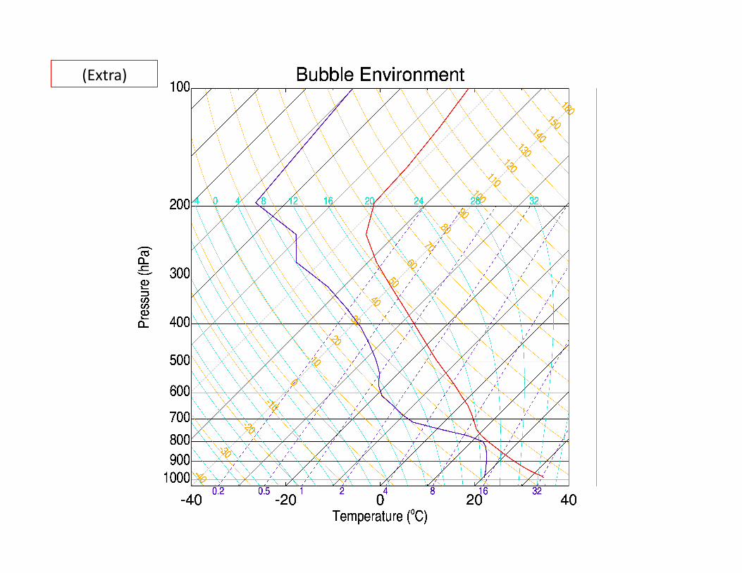
(Extra)


![arXiv:2004.08397v2 [astro-ph.GA] 21 Apr 2020 · 2020-04-22 · 12South African Astronomical Observatories, Observatory, Cape Town 7925, South Africa 13Centre for Astrophysics Research,](https://static.fdocument.org/doc/165x107/5fb71bf143b5d05f7e35cdcf/arxiv200408397v2-astro-phga-21-apr-2020-2020-04-22-12south-african-astronomical.jpg)