Lecture Notes on GeneralRelativity

S. Hollands, Ko Sanders

These lecture notes were prepared by Stefan Hollands, Stefanie Riedel,and Ko Sanders using LATEX 2ε.

2

Preface

These lecture notes on General Relativity intend to give an introduction toall aspects of Einstein’s theory: ranging form the conceptual via the math-ematical to the physical. In the first part we discuss Special Relativity,focusing on the re-examination of the structure of time and space. In thesecond part we cover General Relativity, starting with an introduction to thenecessary mathematical tools and then explaining the structure of the the-ory, the conceptual motivations for it and its relation between spacetime andgravity. Finally, in the third part, we focus on physical applications of Ein-stein’s theory at several length scales: gravitational waves, cosmology, blackholes and GPS. Whereas the third application is the most practical, the firstthree are the best illustration for how General Relativity has influenced ourunderstanding of the world around us.

3

Contents

I Special Relativity 6

1 Introduction 6

2 Time and Space in Classical Mechanics 7

3 Electromagnetism and Poincare Invariance 11

4 Spacetime in Special Relativity 14

5 Mathematics of Minkowski Spacetime 17

6 Mechanics in Special Relativity 21

7 Observer Dependence and Paradoxes 25

II General Relativity 29

8 Introduction 29

9 Mathematical Preliminaries 30

9.1 Calculus of Tensors . . . . . . . . . . . . . . . . . . . . . . . . 31

9.2 Manifolds . . . . . . . . . . . . . . . . . . . . . . . . . . . . . 34

9.3 Tangent, Cotangent and Tensor Bundles . . . . . . . . . . . . 40

9.4 Covariant Derivatives . . . . . . . . . . . . . . . . . . . . . . . 45

9.5 Metrics and Geodesics . . . . . . . . . . . . . . . . . . . . . . 50

10 General Relativity 58

10.1 Kinematics of General Relativity . . . . . . . . . . . . . . . . 58

10.2 Dynamics of General Relativity . . . . . . . . . . . . . . . . . 64

10.3 Properties of General Relativity . . . . . . . . . . . . . . . . . 68

10.4 Stress-Tensor and Energy Conditions . . . . . . . . . . . . . . 71

III Applications of General Relativity 76

4

11 Spacetime Symmetries 76

12 Cosmological Solutions to Einstein’s Equation (MaximallySymmetric Universes) 7912.1 Redshift in cosmological spacetimes . . . . . . . . . . . . . . . 8812.2 Particle Horizons . . . . . . . . . . . . . . . . . . . . . . . . . 92

13 Black Holes 9313.1 Derivation of the Schwarzschild Solution . . . . . . . . . . . . 9413.2 The redshift effect . . . . . . . . . . . . . . . . . . . . . . . . . 9613.3 Geodesics . . . . . . . . . . . . . . . . . . . . . . . . . . . . . 9713.4 Kruskal extension . . . . . . . . . . . . . . . . . . . . . . . . . 102

14 Linearized Gravity and Gravitational Radiation 10714.1 Gravitational waves in empty space . . . . . . . . . . . . . . . 10814.2 Sources of gravitational waves . . . . . . . . . . . . . . . . . . 113

15 The Global Positioning System 11915.1 Introduction . . . . . . . . . . . . . . . . . . . . . . . . . . . . 11915.2 Modelling the gravitational field of Earth . . . . . . . . . . . . 12115.3 Choice of coordinates . . . . . . . . . . . . . . . . . . . . . . . 12315.4 Time measurement on a satellite . . . . . . . . . . . . . . . . . 12515.5 How to synchronise clocks on different satellites. . . . . . . . . 12715.6 Communication with users on Earth . . . . . . . . . . . . . . 12815.7 Conclusions . . . . . . . . . . . . . . . . . . . . . . . . . . . . 129

5

Part I

Special Relativity

1 Introduction

Time and space are two of the most basic concepts in describing the worldaround us. Even young children soon master the difference between ”here”and ”there”, and between ”now” and ”later” or ”earlier”. However, strictlyspeaking, the concepts of time and space are only derived notions, which weintroduce as a theoretical construct to help order our observations of eventsin the world around us.

Because our intuitions about time and space are so strong, it is hardto imagine a description of the world without them, or to explain in detailhow those constructs come about. It should not be surprising, therefore,that time and space were long thought to have a fixed structure, which hasbeen formalised by Newton, Galileo and Leibniz in the early days of modernscience. These notions are now called ”absolute time” and ”absolute space”(or ”absolute distance”). Immanuel Kant could not imagine how time andspace could possibly have any other structure and he even went so far as toraise that structure to a fundamental ordering principle of human thought.

Interestingly, Newton himself noted that absolute time and distance werenot entirely without problems. He illustrated this in the form of the ”ro-tating bucket” paradox. However, this paradox did not seem to admit anyexperimental investigation, so it remained unresolved for a long time anddidn’t diminish the impression that the notions of absolute time and spacewere correct.

It should be considered a major achievement of human thought that thenotions of absolute time and space were found to be faulty and that theycould be replaced by something better: the concept of spacetime. It wasonly possible after Maxwell completed the unification of the theories of elec-tricity and magnetism into a single theory of electromagnetism, based onFaraday’s concept of a field, which avoids action at a distance. Maxwell’stheory brought to light a new problem with the notions of absolute time andspace: the theory was not invariant under all Galilean transformations. Ein-stein1 found that this discrepancy could be resolved in the most elegant way

1Albert Einstein won the 1921 Nobel Prize in physics “for his services to theoretical

6

by noting that the concepts of absolute time and space were not well moti-vated in an operational way. In his Special Theory of Relativity he replacedthem by the new concept of spacetime.

2 Time and Space in Classical Mechanics

For comparison with Special Relativity, it will be useful to give a fairly de-tailed analysis of the structure of time and space in the classical mechanicsof Newton. Let us denote by M the set of all possible events in the universe.Here an event can be identified uniquely by a time and place, indicating whenand where the event happens. We usually encode the time and place intonumbers, which we call coordinates.

To find out when an event p ∈ M happens, we may use a clock: when phappens we read off the time, t(p). In this way the clock defines a function t :M → R. To understand the notion of absolute time, we need to understandhow much of the number t(p) depends on the properties of the clock we use,and how much of it is independent of those properties.

Let us first agree to use an ideal clock: it runs for ever and is not influencedby anything happening around it. (Of course such ideal clocks don’t reallyexist, but they help to clarify the notion of absolute time.) Ideal clocks go along way to exhibit the structure of absolute time, but two ideal clocks maystill give different readings for two reasons:

1. Two ideal clocks can disagree which events happen at t = 0.

2. Two ideal clocks can use different units of time.

In other words, given an ideal clock t : M → R, there is no special physicalsignificance to events p with t(p) = 0, or on the time difference t(p1)− t(p2)for any two events p1, p2. However, all ideal clocks do agree on the following:

Tenet 2.1 (Absolute Time) In classical mechanics, for arbitrary eventsp1, p2, p

′1, p′2 ∈M , all ideal clocks t : M → R agree on

1. whether t(p1) > t(p2), t(p1) < t(p2) or t(p1) = t(p2),

2. the value of t(p1)−t(p2)t(p′1)−t(p′2)

when t(p′1) 6= t(p′2).

physics, and especially for his discovery of the law of the photoelectric effect”.

7

The first property defines a time orientation on M : the notions of before,after and simultaneous are well defined for all events, independent of theideal clock. In the second property, the denominator t(p′1)− t(p′2) essentiallyfixes the units of time. When the units of time are fixed, all ideal clocks agreeon the time interval between any two events. Together these two propertiesfully characterise absolute time. (Note in particular that we can compare theduration of any two time intervals, regardless of when or where the eventsare located.)

Exercise 2.2 Let t : M → R and t′ : M → R be time coordinates defined byideal clocks. Show that t′(p) = rt(p) + t′0 for some r > 0 and t′0 ∈ R.

In an analogous way one may identify places in M using ideal measuringrods, which are infinitely extended and which are not influenced by anyphysical processes happening in the universe. These ideal measuring rodscan be used to form an infinite grid, where the rods intersect at right angles.The grid defines coordinate maps x : M → R3, where x = (x1, x2, x3) incomponents.

For a given absolute time coordinate t we denote by Mt=c the subset ofM of all events taking place at time t = c. All these simultaneous eventsmake up the entire space at the moment t = c. The notion of absolute spacein classical mechanics can then be formulated as follows:

Tenet 2.3 (Absolute Space) In classical mechanics, for any c ∈ R andany events p1, p2, p

′1, p′2 ∈Mt=c, all ideal measuring rods agree on the follow-

ing:

1. the value of ‖x(p1)−x(p2)‖‖x(p′1)−x(p′2)‖ , when ‖x(p′1)− x(p′2)‖ 6= 0,

2. Mt=c is a three-dimensional Euclidean space, i.e. we may construct agrid of ideal measuring rods such that the distance between p1 and p2

satisfies Pythagoras’ Theorem

‖x(p1)− x(p1)‖ =

√√√√ 3∑i=1

(xi(p1)− xi(p2))2.

Again the origin of the coordinates x does not have any physical significance,nor does the orientation. The first property means that all ideal grids agreeon the (absolute) distances, up to a change of units. The second propertyfixes the global shape of space Mt=c.

8

Exercise 2.4 For fixed c ∈ R, let x : Mt=c → R3 and x′ : Mt=c → R3 bebijections, such that

‖x′(p1)− x′(p2)‖‖x′(p′1)− x′(p′2)‖

=‖x(p1)− x(p2)‖‖x(p′1)− x(p′2)‖

for all p1, p2, p′1, p′2 ∈Mt=c with ‖x′(p′1))− x′(p′2))‖ 6= 0. Show that

x′(p) = rA · x(p) + x′0

for some x′0 ∈ R3 and some orthogonal matrix A and some r > 0. (Hint:first identify x′0 and r > 0. Then consider the map ψ : R3 → R3 : X 7→r−1(x′ x−1(X) − x′0). Using the real polarisation identity for the standardinner product, 2〈X, Y 〉 = ‖X‖2 + ‖Y ‖2 − ‖X − Y ‖2 for all X, Y ∈ R3, showthat ψ must preserve the inner product, because it preserves all distances.Use this to prove that ψ is linear and to find A.)

We can use an ideal clock and an orthogonal grid of ideal measuring rodsto define a coordinate system (t,x) : M → R4. In this way, each event in Mis assigned a unique set of coordinates. Coordinates which are obtained inthis way are called classical inertial coordinates. The following is a centraltenet of classical mechanics:

Tenet 2.5 (Galilean Relativity Principle) In all classical inertial coor-dinate systems, the physics of classical mechanics is described by Newton’slaws in terms of absolute time and distance.

In other words, the classical inertial coordinate systems form a preferred classof coordinate systems and Newton’s laws are invariant under the change ofcoordinates from one classical inertial coordinate system to another. How-ever, within classical mechanics, no classical inertial coordinate system ispreferred over any other, simply because one cannot distinguish them by anyexperimental procedure satisfying Newton’s laws. E.g., (approximate) clas-sical inertial coordinates attached to the Earth are no better or worse thanthe (approximate) classical inertial coordinates attached to a train movingwith a constant velocity in a fixed direction. Our natural intuition to favourthe first coordinate system, which is more familiar, cannot be justified byclassical mechanics.

9

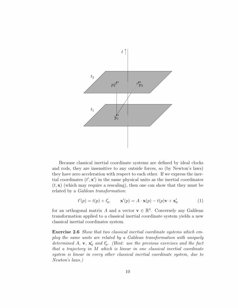
t1

t2

p1

p2 p3

t

Because classical inertial coordinate systems are defined by ideal clocksand rods, they are insensitive to any outside forces, so (by Newton’s laws)they have zero acceleration with respect to each other. If we express the iner-tial coordinates (t′,x′) in the same physical units as the inertial coordinates(t,x) (which may require a rescaling), then one can show that they must berelated by a Galilean transformation:

t′(p) = t(p) + t′0, x′(p) = A · x(p)− t(p)v + x′0 (1)

for an orthogonal matrix A and a vector v ∈ R3. Conversely any Galileantransformation applied to a classical inertial coordinate system yields a newclassical inertial coordinates system.

Exercise 2.6 Show that two classical inertial coordinate systems which em-ploy the same units are related by a Galilean transformation with uniquelydetermined A, v, x′0 and t′0. (Hint: use the previous exercises and the factthat a trajectory in M which is linear in one classical inertial coordinatesystem is linear in every other classical inertial coordinate system, due toNewton’s laws.)

10

Exercise 2.7 Show that the Galilean transformations form a group (i.e. thecomposition and the inverses of such transformations are Galilean transfor-mations).

Exercise 2.8 Let (t,x) be classical inertial coordinates and let p1 and p2 bethe events such that x(p1) = x(p2), but t(p2) > t(p1). Does it make sense tosay that the event p2 happens at the same place as p1 but at a later time?(I.e. would all inertial coordinate systems agree that p2 is at the same placeas p1?) Do points of space preserve their identity in the course of time?

Example 2.9 (Rotating bucket paradox) Let (t,x) be a classical iner-tial coordinate system and consider new coordinates (t′,x′) which rotate arounda fixed axis with a constant angular velocity, e.g.:

t′(p) = t(p), x′(p) = Rt(p) · x(p),

where Rt(p) is a rotation around the x3-axis over an angle t(p). Note that(t′,x′) is not a classical inertial coordinate system. Expressing physical lawsin the coordinates (t′,x′) leads to different formulae than in the coordinates(t,x) (including a centrifugal force).

Newton already noted that a bucket of water in an otherwise empty uni-verse, which stands still w.r.t. the coordinates (t′,x′), rotates w.r.t. (t,x).The water in the bucket experiences a centrifugal force, which causes it torise against the walls of the bucket. Without rotation, the water would re-main flat. Note that the difference cannot be caused by any other matter inthe universe, so it must be due to rotations w.r.t. empty space. This effectis surprising, because a rotation w.r.t. empty space is difficult to see. Thisproblem is called ”Newton’s rotating bucket paradox”.

3 Electromagnetism and Poincare Invariance

A first modification of our understanding of time and space was initiatedwhen Maxwell completed the unification of the theories of electricity andmagnetism. The theory of electromagnetism concerns an electric field E anda magnetic field B on the spacetime M , which satisfy Maxwell’s equationsof motion. In vacuum these equations take the form

∇× E = −∂tB, ∇ ·B = 0

∇ · E = 0, ∇×B =1

c2∂tE. (2)

11

expressed in inertial coordinates (t,x) fixed to Earth.One of the nice aspects of Maxwell’s theory of electromagnetism is that

it is a field theory2, which implements the intuition that physical influencesshould propagate from point to neighbouring point. Indeed, Maxwell’s equa-tions imply that all components of E and B satisfy the wave equation:

2E := − 1

c2∂2t E + ∆E = 0, (3)

where ∆ :=∑3

i=1 ∂2xi is the Laplace operator and 2 is called the d’Alembert

operator. This equation ensures that disturbances in the (components of the)fields can propagate no faster than a certain maximum speed c, the speed oflight in vacuum.

Maxwell’s equations have another property, however, which seems verypuzzling in comparison to classical mechanics: the equations are not invariantunder all Galilean transformations. Although there is no problem with trans-lations or rotations in space, the equations are not invariant under uniformmotion. In particular, the speed of light in vacuum follows from Maxwell’sequations, so if these equations were invariant, all inertial coordinate systemswould have to agree on this speed. However, for a coordinate system movingfast in the opposite direction of a light ray, one might expect the (relative)speed of that light ray to be bigger!

Exercise 3.1 Consider a Galilean transformation to a coordinate system(t′,x′) which moves at a constant speed v in the x1 direction. Show that thewave equation (3) transforms to the equation

2′E = v2∂2x′E + 2v∂t′∂x′E,

where 2′ is defined in a similar way as 2, but with respect to the new coor-dinates. Show in a similar way that Maxwell’s equations transform to

∇′ × E = −∂t′B− v∂x′B, ∇′ ·B = 0

∇′ · E = 0, ∇′ ×B =1

c2(∂t′E + v∂x′E).

so Maxwell’s equations are not invariant under this Galilean transformation.(This conclusion remains true, even if we argue that the components of E

2The concept of a field is due to Faraday.

12

and B are components of vectors, so they should also transform under thechange of coordinates. We will see in Section 9.1 that several componentsof the fields should be unaffected by the change of coordinates, but the waveequation for those coordinates is not invariant.)

The mathematical modifications needed to reconcile electromagnetismwith absolute time and space were soon understood: Maxwell’s equationsare invariant under Poincare transformations :

t′(p) = γ(t(p)− c−2v(A · x(p))‖

)+ t′0,

x′(p) = (A · x(p))⊥ + γ((A · x(p))‖ − t(p)v

)n + x′0 (4)

γ := (1− c−2‖v‖2)−12 ,

where A is an orthogonal matrix, v = vn a velocity vector with speedv = ‖v‖ < c, and ‖ and ⊥ denote the components of a vector parallel orperpendicular to the unit vector n. When v = 0 the two transformationscoincide, but for uniform motion this is not so. When the inhomogeneousterms t′0 and x′0 vanish, we speak of a Lorentz transformation. Lorentz trans-formations for which A = I are called boosts with relative velocity v 6= 0.

Exercise 3.2 Show that any Poincare transformation can be written as acomposition of an orthogonal transformation A of the spatial coordinates, aboost with relative velocity v and a translation in spacetime along (t′0,x

′0).

Show that A, v and (t′0,x′0) are uniquely determined.

Exercise 3.3 Show that the wave equation (3) is invariant under Poincaretransformations. (Hint: by the previous exercise it suffices to consider or-thogonal transformations, boosts and translations.)

Exercise 3.4 Consider a boost with relative velocity v and find the 4 × 4matrix L such that (

t′

x′

)= L ·

(tx

).

Consider the limit c → ∞ with c−1x0 remaining finite and show that onerecovers a Galilean transformation.

One may argue that electromagnetism enables us to do experiments whichgo beyond classical mechanics and which allow us to distinguish certain in-ertial reference frames from others. However, there are several objections

13

to this argument. Firstly, by Galilean Invariance the speed of light shoulddiffer for classical inertial coordinates moving in different directions, but thefamous Michelson-Morley experiment3 failed to detect such differences. Sec-ondly, classical mechanics describes the motion of rigid bodies whose internalforces and collision forces are predominantly electromagnetic. In a uniformlymoving frame at velocity v, Maxwell’s equations take a different form, allow-ing us to detect v. It would be very remarkable if in some miraculous waythe effect of electromagnetism on rigid bodies should cancel out completelyto ensure that the Galilean Relativity Principle is satisfied.

Einstein realised that the conflict of classical mechanics with electromag-netism can be resolved most elegantly by noting that the notions of absolutetime and distance are not operationally justified and need modification. E.g.,let p1, p2 ∈ M be two events which are supposedly simultaneous, but sepa-rated by a large distance. To verify that they really are simultaneous, onewould need to be able to communicate between the places where the eventsare taking place at arbitrarily high speeds. Certainly no electromagneticcommunication channel could satisfy this, because electromagnetic signalstravel at a finite speed of propagation.

In his Special theory of Relativity, Einstein took electromagnetism asmore fundamental than the notions of absolute time and distance, and hedeclared the speed of light in vacuum to be a universal physical constant.This forced him to weaken the assumptions on the properties of time andspace, leading to the new concept of spacetime, which we investigate next.

4 Spacetime in Special Relativity

Let xµ be coordinates on M , where µ = 0, . . . 3 and x0 := ct, and supposethat Newton’s first law and Maxwell’s equations are both valid in these co-ordinates. We call these coordinates (relativistic) inertial coordinates, or a(relativistic) inertial frame. (That such coordinates exist, to a high degreeof accuracy, is known from experience.) Now let x′µ be any new set of co-ordinates, obtained from xµ by a Poincare transformation. Then Maxwell’sequations will also hold in the new coordinates, and so will many essentialaspects of Newton’s laws, because the change of coordinates is linear. In

3Albert Michelson won the 1907 Nobel Prize in physics “for his optical precision in-struments and the spectroscopic and metrological investigations carried out with theiraid”.

14

particular, the straight paths of free particles will map to straight paths,which means that the new coordinates are also inertial coordinates. How-ever, two sets of inertial coordinates may no longer agree on time differencesbetween all events or on the question whether two events are simultaneous,let alone on the distance between simultaneous events, masses of particlesor the strengths of forces. This means that Newtonian mechanics will needsome modification.

In order to preserve the equations of electromagnetism and (much of)classical mechanics, Einstein proposed to remove absolute time and distancefrom Galileo’s Relativity Principle:

Tenet 4.1 (Special Relativity Principle) In all inertial coordinate sys-tems, the physics of classical mechanics and of electromagnetism are describedrespectively by (an adaptation of) Newton’s laws and Maxwell’s equations. Inaddition, nothing moves faster than c, the speed of light in vacuum.

Despite the absence of absolute time and distances, there are still somestatements that all inertial coordinate systems agree on. To formulate these,we introduce a standard basis on R4, eµ with µ = 0, . . . , 3, so we may writex =

∑3µ=0 x

µeµ. In addition we introduce a bilinear symmetric form on R4,

η(x, y) := −x0y0 + (x1y1 + x2y2 + x3y3), (5)

which is called the Lorentz inner product (or rather, pseudo-inner product).Note that η(x, x) is not always non-negative, but η is non-degenerate: whenη(x, y) = 0 for all y, then x = 0. We say that x, y ∈ R4 are orthogonal whenη(x, y) = 0.

We define the spacetime interval (in appropriate units) by

σ(p1, p2) := η(x(p1)− x(p2), x(p1)− x(p2)). (6)

When a physical signal travels from event p1 to event p2, then

σ(p1, p2) = −(x0(p1)− x0(p2))2 + ‖x(p1)− x(p2)‖2 ≤ 0,

x0(p2)− x0(p1) ≥ 0,

because the signal cannot travel faster than the speed of light c. We haveequality in the first line exactly when the signal travels at the speed of lightand along a straight line.

15

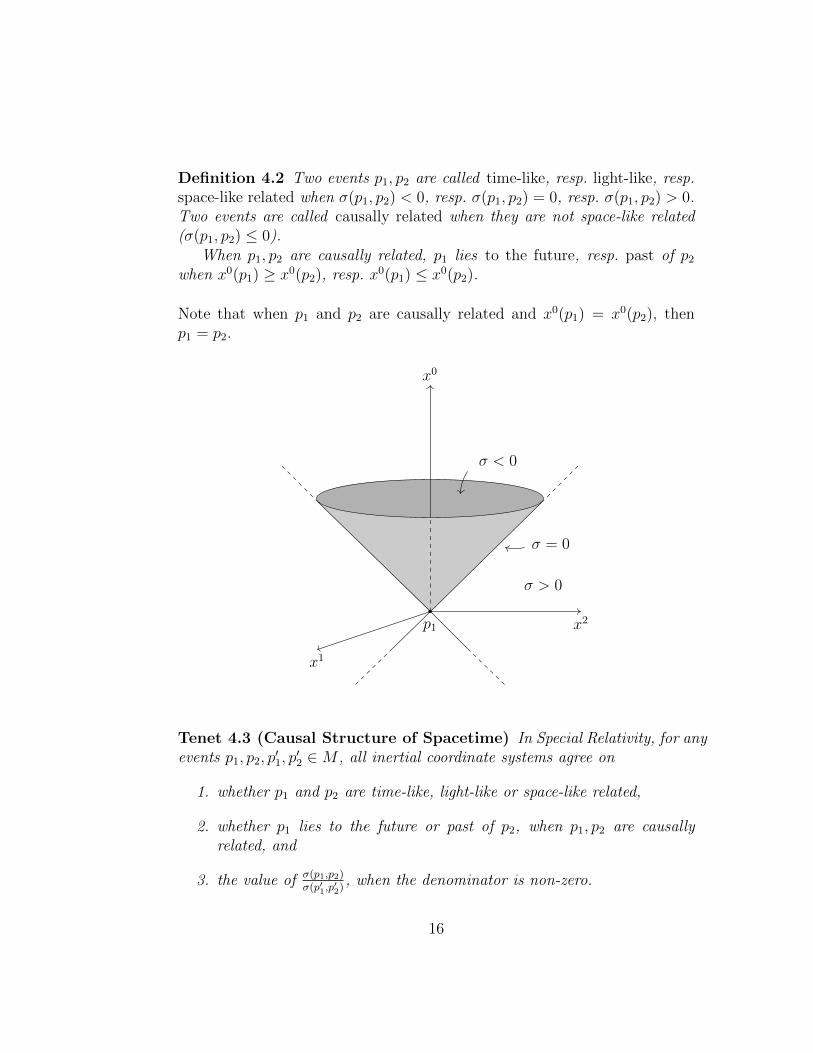
Definition 4.2 Two events p1, p2 are called time-like, resp. light-like, resp.space-like related when σ(p1, p2) < 0, resp. σ(p1, p2) = 0, resp. σ(p1, p2) > 0.Two events are called causally related when they are not space-like related(σ(p1, p2) ≤ 0).

When p1, p2 are causally related, p1 lies to the future, resp. past of p2

when x0(p1) ≥ x0(p2), resp. x0(p1) ≤ x0(p2).

Note that when p1 and p2 are causally related and x0(p1) = x0(p2), thenp1 = p2.

x0

x1

x2p1

σ > 0

σ < 0

σ = 0

Tenet 4.3 (Causal Structure of Spacetime) In Special Relativity, for anyevents p1, p2, p

′1, p′2 ∈M , all inertial coordinate systems agree on

1. whether p1 and p2 are time-like, light-like or space-like related,

2. whether p1 lies to the future or past of p2, when p1, p2 are causallyrelated, and

3. the value of σ(p1,p2)σ(p′1,p

′2)

, when the denominator is non-zero.

16

The second statement means that all inertial coordinate systems agree on thetime-ordering between any two causally related events. In the last statement,the denominator is once again used to fix units. Note that in Special Rel-ativity it suffices to fix time units only, because corresponding spatial unitsare then obtained by multiplication with the universal constant c.

Exercise 4.4 Show that Poincare transformations preserve the spacetimeinterval σ and the causal structure of Tenet 4.3.

Note that we have not defined simultaneity between events. In SpecialRelativity such a notion can only be defined in a coordinate dependent way.

One might worry that the choice of an inertial coordinate system xµ isalready more than can be justified in an operational way. E.g., if an observerremains at position x = 0, how can he possibly ascribe coordinates to eventswith x 6= 0, or synchronise watches at different places? The answers to suchquestions were elaborated by Einstein in an entirely operational way, usingonly light signals and their reflections. This means that inertial coordinatescan be constructed by a procedure that is independent of the observer, andfor any two observers the resulting sets of inertial coordinates are indeedrelated by a Poincare transformation. For the details of these procedures werefer to interested reader to most text books on Special Relativity.

5 Mathematics of Minkowski Spacetime

Using inertial coordinates xµ we identify M with R4 and the structure ofspacetime is then entirely encoded in η. The pair (R4, η) is called Minkowskispace (or rather: Minkowski spacetime). We will now formulate the struc-ture of M and of the Poincare transformations systematically in this four-dimensional formulation, using the coordinates xµ. Most of the results areformulated in terms of exercises.

The terminology for causal relations on spacetime M can also be usedon R4, using the identification via inertial coordinates. E.g. we say that avector x ∈ R4 is time-like when η(x, x) < 0. (This is equivalent to sayingthat the event in M corresponding to the coordinates x is time-like relatedto the event corresponding to the coordinates 0 ∈ R4.) Similarly, x is futurepointing when it is causal (i.e. η(x, x) ≤ 0) and x0 ≥ 0. In addition we callthe set of all light-light vectors the light cone and the set of all causal vectors

17

the causal cone. These cones can be split up into the forward and backwardcones (each containing the vector 0).

Exercise 5.1 Give a sketch of R4, indicating the sets of space-like vectorsand time-like vectors. Also indicate the forward and backward light cones andcausal cones.

Exercise 5.2 Recall the standard basis eµ of R4, such that x =∑3

µ=0 xµeµ.

Show that

η(eµ, eν) =

−1 µ = ν = 01 µ = ν 6= 00 µ 6= ν

.

Exercise 5.3 Let x ∈ R4 be a time-like vector. Show that all vectors orthog-onal to x (w.r.t. the Lorentz inner product η) are space-like or zero.

Exercise 5.4 Let x, y ∈ R4 be two future pointing causal vectors. Showthat η(x, y) ≤ 0, that z := x + y is a future pointing causal vector and thatη(x, y) = 0 if and only if z is light-like if and only if x and y are light-likeand parallel to each other.

Exercise 5.5 Find all vectors in R4 which are orthogonal to themselves(w.r.t. the Lorentz inner product η).

We will now focus on Poincare transformations.

Exercise 5.6 Show that any Poincare transformation is of the form

x′µ(p) = L · xµ(p) + x′µ0 ,

for a unique x′0 ∈ R4 and a unique 4× 4-matrix L such that

η(L · x, L · y) = η(x, y)

for all x, y ∈ R4. Express L in terms of A and v of Ex. 3.2.

Exercise 5.7 Show that the Poincare transformations form a group.

Exercise 5.8 Show that two inertial coordinate systems which employ thesame units are related by a Poincare transformation.

18

It is sometimes helpful to also introduce the standard Euclidean innerproduct 〈x, y〉 =

∑3µ=0 x

µyµ. Any elements x, y ∈ R4 then have

η(x, y) = 〈x, η · y〉

for the diagonal matrix

η :=

−1 0 0 00 1 0 00 0 1 00 0 0 1

. (7)

Note, however, that the standard basis or inner product have no special phys-ical significance. (They are not invariant under Poincare transformations.)

The 4×4-matrices satisfying η(L ·x, L ·y) = η(x, y) form a (Lie-)group L,called the Lorentz group. Equivalently, it consists of all matrices satisfyingLT · η · L = η. Any element L ∈ L has detL = ±1 and, expressed in thebasis eµ, the entry L00 6= 0, because

−L200 +

3∑i=1

L2i0 = 〈L · e0, η · L · e0〉 = 〈e0, η · e0〉 = −1.

We may therefore decompose L into the four disjoint subsets (which are notnecessarily subgroups)

L↑+ = L ∈ L| detL = +1, L00 > 0,L↑− = L ∈ L| detL = −1, L00 > 0,L↓+ = L ∈ L| detL = +1, L00 < 0,L↓− = L ∈ L| detL = −1, L00 < 0.

One may show that all these subsets are connected. We can go from any ofthese subsets to any other by multiplication with one of the following specialelements:

• parity operation (”spatial reflection”): L = −η,

• time reversal operation: L = η,

• spacetime reflection: L = −I.

19

Exercise 5.9 Show that L ∈ L defines a Lorentz transformation (whichpreserves the causal structure of Tenet 4.3) if and only if L is in the or-thochronous Lorentz group

L↑ := L↑+ ∪ L↑−.

Other subgroups of L are the proper Lorentz group L+ = L ∈ L| detL =+1 and the proper, orthochronous Lorentz group L↑+. (The latter wouldhave been the group of interest if we had also introduced an orientation onMinkowski spacetime, in addition to the time orientation.)

Exercise 5.10 Let x ∈ R4 be a future pointing time-like vector. Show thatthere is a matrix L ∈ L such that L · x = e0, the standard basis vector whichis future pointing and time-like.

In the remaining part of this section we give some exercises about boosts,which illustrate the sometimes counter-intuitive consequences of the absenceof absolute time.

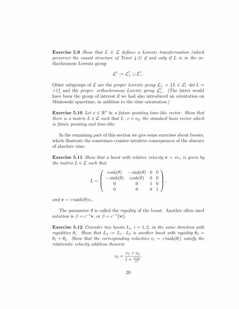
Exercise 5.11 Show that a boost with relative velocity v = ve1 is given bythe matrix L ∈ L such that

L =

cosh(θ) − sinh(θ) 0 0− sinh(θ) cosh(θ) 0 0

0 0 1 00 0 0 1

,

and v = c tanh(θ)e1.

The parameter θ is called the rapidity of the boost. Another often usednotation is β = c−1v, or β = c−1‖v‖.

Exercise 5.12 Consider two boosts Li, i = 1, 2, in the same direction withrapidities θi. Show that L3 := L1 · L2 is another boost with rapidity θ3 =θ1 + θ2. Show that the corresponding velocities vi = c tanh(θi) satisfy therelativistic velocity addition theorem

v3 =v1 + v2

1 + v1v2c2

.

20

6 Mechanics in Special Relativity

Let us now explain how classical mechanics can be reformulated in the contextof Special Relativity. The trajectory that any point-like object follows in thecourse of time forms a curve in the spacetime M , which is called a world line.We begin this section by considering curves in M .

Let I = (a, b) ⊂ R be an open interval and consider a (parameterised)curve ξ : I →M . We choose some inertial coordinate system xµ to make anidentification X : M → R4, so that X(ξ(s)) =

∑3µ=0 ξ

µ(s)eµ with coordinates

ξµ := xµ ξ. We also assume that the ξµ are C1 (continuously differentiable)and we denote the derivatives w.r.t. the parameter s ∈ I by a dot, e.g. ξµ(s).We will also write ξ(s) :=

∑3µ=0 ξ

µ(s)eµ. Curves are a natural way to modelthe trajectories of particles or other physical objects.

We may distinguish several kinds of curves, which have a definite causalcharacter and time orientation:

Definition 6.1 A C1 curve ξ : I → M is called space-like, resp. light-like,resp. time-like, resp. causal, when for all s ∈ I, η(ξ(s), ξ(s)) > 0, resp.η(ξ(s), ξ(s)) = 0, resp. η(ξ(s), ξ(s)) < 0, resp. η(ξ(s), ξ(s)) ≤ 0.

A causal C1 curve ξ is future, resp. past directed when for all s ∈ I,ξ0(s) ≥ 0, resp. ξ0(s) ≤ 0.

Now consider a C1 bijection s : I ′ → I with a C1 inverse, where I ′ =(a′, b′). We call the curve ξ′ : I ′ → M defined by ξ′(s′) := ξ(s(s′)) areparametrisation of ξ. The image of ξ′ coincides with the image of ξ. Thespeed with which this image is traced out may differ, but the velocity vectorsare always parallel:

ξ′µ(s′) = ξµ(s(s′))∂s′s(s′).

We say that ξ′ has the same direction as ξ when s : I ′ → I preserves theorientation, i.e. when s(a′) < s(b′). Otherwise we say that ξ′ has the oppositedirection as ξ.

Exercise 6.2 Show that the causal character (space-like, light-like, time-likeor causal) of a C1 curve is independent of the choice of the parametrisa-tion. Show that the time-orientation of a causal curve is preserved when thereparametrisation preserves the direction of the curves.

Exercise 6.3 All curves in this exercise are assumed to have C1 coordinates:

21

1. Find a curve which is neither space-like nor causal.

2. Find a spacelike curve ξ : (−2, 2) such that ξ(1) lies to the future ofξ(−1).

3. Find a causal curve which is neither light-like not time-like.

4. Find a causal curve which is neither future nor past directed.

5. Show that every time-like curve is either future or past directed.

In analogy to the length of a curve in Euclidean geometry, we can definethe arc length of a space-like C1 curve by:

l(ξ) :=

ˆI

√η(ξ(s), ξ(s))d s

For a causal C1 curve we similarly define the proper time to be

τ(ξ) :=1

c

ˆI

√−η(ξ(s), ξ(s))d s.

Using the arc length and proper time we may find preferred parametrisationsfor all causal and space-like C1 curves:

Definition 6.4 A C1 space-like curve is parameterised by arc-length whenη(ξ, ξ) = 1.

A C1 time-like curve is parameterised by proper time when η(ξ, ξ) = −c2.

Theorem 6.5 A space-like curve ξ can always be parameterised by arc-length, without changing its direction. A time-like curve ξ can always be pa-rameterised by proper time, without changing its direction (or time-orientation).These parametrisations are independent of the choice of inertial coordinates(up to a choice of units).

Proof: In the space-like case we may choose s′(s) such that ∂ss′(s) =√

η(ξ(s), ξ(s)) and in the time-like case such that ∂ss′(s) = 1

c

√−η(ξ(s), ξ(s)).

In this way we find orientation preserving changes of parameter and it isstraight-forward to check that they implement the desired conditions. Inde-pendence of the choice of inertial coordinates follows from the independenceof the spacetime interval (up to a choice of units). 2

22

Exercise 6.6 Show that the arc length and proper time are independent ofthe choice of coordinates xµ and of the parametrisation of ξ. This showsthat the parametrisations by arc length or proper time are independent of thechoice of inertial coordinates.

When a future directed time-like curve ξ(τ) is parameterised by propertime, we may define its velocity and acceleration as:

ξ(τ) :=3∑

µ=0

ξµ(τ)eµ,

ξ(τ) :=3∑

µ=0

ξµ(τ)eµ.

The expressions on the left are independent of the choice of inertial coordi-nates, if we let a change of coordinates also affect the basis eµ. By the (rest)mass m0 of a particle we mean the mass that it has in an inertial coordinatesystem where it is at rest, i.e. a frame where it maintains a fixed positionin space, so that it follows the trajectory τ 7→ (cτ,x0) for some fixed x0.When such a particle traverses a general, future directed, time-like curve ξ,we define its energy-momentum vector to be

P µ(τ) := m0ξµ(τ), (8)

where τ is the proper time of the curve. In Special Relativity, Newton’s firstlaw then takes the form

F µ(τ) = ∂τPµ(τ) (9)

Let us now fix any choice of inertial coordinates and express the formulaeabove in terms of the coordinate time x0, rather than the proper time τ .If a curve is time-like, then ξ0(s) 6= 0 for all s ∈ I and (after reversing theorientation of the parameter, if necessary) we may assume that ξ0(s) > 0. Wemay then introduce a new parameter t, defined by t(s) := c−1

´ ss0ξ0 for some

s0 ∈ I. (The map s 7→ t(s) will be an orientation preserving diffeomorphismon I, because ξ0 > 0.) The new parametrisation leads to

ξ0(s) = ∂sξ′0(t(s)) = ξ′0(t)t(s)

and hence ξ′0(t) = c. This means that, after changing parametrisation, wemay assume that ξ0(t) = ct and ξµ(t) = (ct,x(t)).

23

The parameter derivative is now the same as the time derivative w.r.t.the inertial time coordinate t = c−1x0:

ξµ(t) = (c, x(t)) =: (c,v(t)).

The formula above then shows that (in an arbitrary choice of inertial coordi-nates) the speed of the time-like curve satisfies ‖v(t)‖ < c. This shows thattime-like, future pointing curves model the trajectories of massive particles(also in the presence of forces). When ξ is a light-like curve (but ξ 6= 0)we find in a similar way that ‖v(t)‖ = c, which models the trajectory of amassless particle or light ray. Similarly, space-like curves may have speeds‖v(t)‖ > c, or even infinite speeds. Such curves do not model any knownmatter in the universe. Hypothetical particles that move faster than lightare called tachyons.

A comparison of the parametrisation ξµ(t) with the parametrisation byproper time yields:

ξµ(τ) = ∂τ t(τ)ξµ(t(τ)) = γ(τ) (c,v(t(τ))) ,

∂τ t(τ) = γ(τ) := (1− c−2‖v(t(τ))‖2)−12 ,

where the second line follows from the normalisation c2 = −η(ξµ(τ), ξµ(τ)).It follows that

P µ(τ) = m0γ(τ)ξµ(t(τ)) = m0γ(τ) (c,v(t(τ))) =: (c−1E(t(τ)),P(t(τ))),

so that spatial components of the energy-momentum vector P µ(τ) in thegiven inertial frame take the form P(t) = m(t)v(t), where the apparent (orinertial) mass in this coordinate frame is m(t) = γ(τ(t))m0. (Note that ahigh velocity implies a high apparent mass.) The energy in the given inertialframe satisfies

E(t) = γ(τ(t))m0c2 = m0c

2 +m0‖v(t)‖2

2+ . . . ,

where we made a Taylor expansion in c−1‖v‖. From this we see that thetotal energy in the given coordinate frame consists not only of the kineticenergy, but also a contribution from the rest mass m0c

2 and higher ordercorrections. Note that the total energy is frame dependent: in the rest frameof the particle, only the first term remains.

24

Taking a further derivative we find

F µ(τ) = ∂τPµ(τ) = γ(τ)

(c−1∂tE(t(τ)), ∂tP(t(τ))

)= γ(τ)

(c−1∂tE(t(τ)),F(t(τ))

),

where F(t) = ∂tP(t) corresponds to the force appearing in Newton’s secondlaw (with a time-dependent mass m(t)) in the given inertial frame.

7 Observer Dependence and Paradoxes

To conclude we present some examples of effects in Special Relativity whichare counter-intuitive and whose resolution relies on the fact that some of thequantities used are defined in a coordinate dependent way.

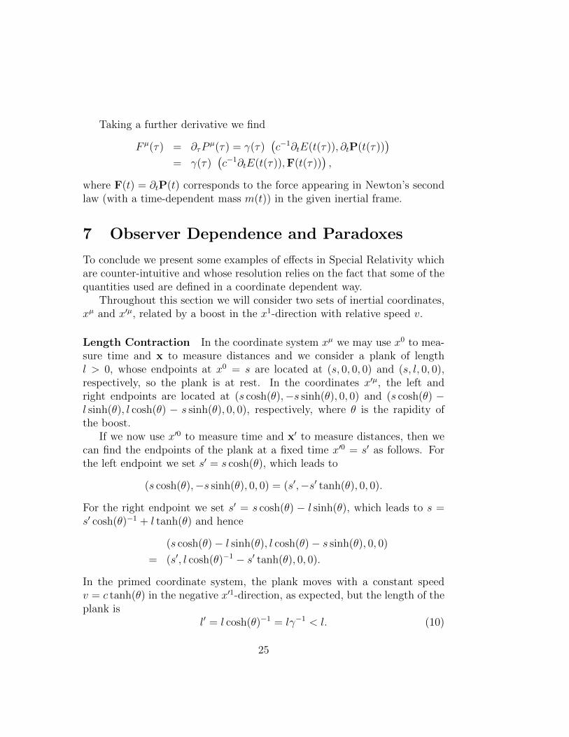
Throughout this section we will consider two sets of inertial coordinates,xµ and x′µ, related by a boost in the x1-direction with relative speed v.

Length Contraction In the coordinate system xµ we may use x0 to mea-sure time and x to measure distances and we consider a plank of lengthl > 0, whose endpoints at x0 = s are located at (s, 0, 0, 0) and (s, l, 0, 0),respectively, so the plank is at rest. In the coordinates x′µ, the left andright endpoints are located at (s cosh(θ),−s sinh(θ), 0, 0) and (s cosh(θ) −l sinh(θ), l cosh(θ) − s sinh(θ), 0, 0), respectively, where θ is the rapidity ofthe boost.

If we now use x′0 to measure time and x′ to measure distances, then wecan find the endpoints of the plank at a fixed time x′0 = s′ as follows. Forthe left endpoint we set s′ = s cosh(θ), which leads to

(s cosh(θ),−s sinh(θ), 0, 0) = (s′,−s′ tanh(θ), 0, 0).

For the right endpoint we set s′ = s cosh(θ) − l sinh(θ), which leads to s =s′ cosh(θ)−1 + l tanh(θ) and hence

(s cosh(θ)− l sinh(θ), l cosh(θ)− s sinh(θ), 0, 0)

= (s′, l cosh(θ)−1 − s′ tanh(θ), 0, 0).

In the primed coordinate system, the plank moves with a constant speedv = c tanh(θ) in the negative x′1-direction, as expected, but the length of theplank is

l′ = l cosh(θ)−1 = lγ−1 < l. (10)

25

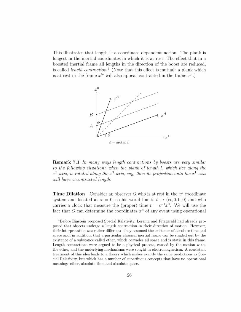
This illustrates that length is a coordinate dependent notion. The plank islongest in the inertial coordinates in which it is at rest. The effect that in aboosted inertial frame all lengths in the direction of the boost are reduced,is called length contraction.4 (Note that this effect is mutual: a plank whichis at rest in the frame x′µ will also appear contracted in the frame xµ.)

x1

x0

x′0

x′1

A

B

φ

φ

φ = arctan β

Remark 7.1 In many ways length contractions by boosts are very similarto the following situation: when the plank of length l, which lies along thex1-axis, is rotated along the x3-axis, say, then its projection onto the x1-axiswill have a contracted length.

Time Dilation Consider an observer O who is at rest in the xµ coordinatesystem and located at x = 0, so his world line is t 7→ (ct, 0, 0, 0) and whocarries a clock that measure the (proper) time t = c−1x0. We will use thefact that O can determine the coordinates xµ of any event using operational

4Before Einstein proposed Special Relativity, Lorentz and Fitzgerald had already pro-posed that objects undergo a length contraction in their direction of motion. However,their interpretation was rather different: They assumed the existence of absolute time andspace and, in addition, that a particular classical inertial frame can be singled out by theexistence of a substance called ether, which pervades all space and is static in this frame.Length contractions were argued to be a physical process, caused by the motion w.r.t.the ether, and the underlying mechanisms were sought in electromagnetism. A consistenttreatment of this idea leads to a theory which makes exactly the same predictions as Spe-cial Relativity, but which has a number of superfluous concepts that have no operationalmeaning: ether, absolute time and absolute space.

26

procedures (involving sending light rays), so he may use x0 as a global timecoordinate.

Now we consider a similar observer O′ in the x′µ coordinate system, sothat each observer sees the other one moving away with a speed v. LetA = (ct1, 0, 0, 0) and B = (ct2, 0, 0, 0) be two events in the coordinates xµ,which differ by a time interval (t2 − t1) according to O. We may expressthese events in the coordinate frame x′µ as

A = (ct1 cosh(θ),−ct1 sinh(θ), 0, 0), B = (ct2 cosh(θ),−ct2 sinh(θ), 0, 0)

in the primed coordinate system. According to O′, the two events are there-fore separated by a time interval

T ′ = cosh(θ)(t2 − t1) = γT, (11)

where T = t2 − t1. According to O′, more time has elapsed between the twoevents, so O’s clock is slow. In a similar way, O will find that the clock thatO′ uses is slow!

This effect is called time dilation. The fact that both observers find theother observer’s clock to be slow violates the intuition that one clock must befaster than the other. However, this intuition is based on the false assumptionthat there exists an absolute time (and that both clocks run at a fixed ratecompared with absolute time).

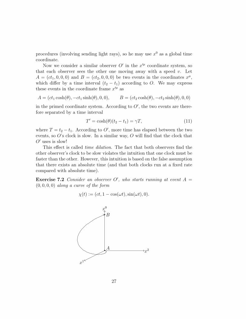
Exercise 7.2 Consider an observer O′, who starts running at event A =(0, 0, 0, 0) along a curve of the form

χ(t) := (ct, 1− cos(ωt), sin(ωt), 0).

x2

x0

x1

A

B

27

For what values of ω is this curve time-like? For what values of ω is O′

also present at the event B = (ct1, 0, 0, 0)? What is the proper length of thiscurve between A and B? For what values of ω is this proper time less thanhalf of the proper time t1 along the straight line t 7→ (ct, 0, 0, 0)? How fastmust O′ run to age only half as fast?

The Twin Paradox Consider the same Observer O in the coordinatesystem xµ and an observer O′ traveling through A = (ct1, 0, 0, 0) to B =(ct2, 0, 0, 0) via any C1 time-like and future pointing curve ξ : I →M . Thenthe following holds:

Theorem 7.3 Let τξ(A,B) be the proper time interval between A and Balong ξ. Then τξ(A,B) ≤ (t2 − t1), with equality if and only if the (proper)velocity satisfies ξµ ≡ (c, 0, 0, 0) between A and B.

Proof: Because ξ is time-like and future pointing we have ξ0(s) > 0 for alls ∈ I, so we may change the parametrisation such that t = c−1x0 becomesthe new parameter and ξµ(t) = (ct,x(t)). The proper time interval betweenA and B is then

τξ(A,B) = c−1

ˆ t2

t1

√c2 − ‖x(t)‖2d t

≤ c−1

ˆ t2

t1

c = (t2 − t1),

which proves the estimate. Note that we have equality if and only if x ≡ 0,which means that ξµ = (c, 0, 0, 0). In that case t is the proper time coordinatealong ξ and we have ξµ(t) = (ct, 0, 0, 0), so ξ does indeed go from A to B. 2

Theorem 7.3 is completely analogous to the familiar result in Euclidean spacethat two points A and B can be connected by curves of different lengths,and there is a unique shortest curve. However, in the present context, theinterpretation of the theorem is that the observer O, who followed the linearcurve, has aged more than the observer O′, who followed the curve ξ. Thisexhibits a violation of the idea of absolute time. The effect is most strikingwhen O′ first travels away from O at a constant speed and then turns aroundto return. ξ is then also a linear curve most of the way, so in view of timedilation, which is symmetric, it is then paradoxical that both observers agreeon the fact that O has aged more than O′.

28

The resolution of the paradox lies in the fact that we cannot (in general)choose an inertial frame in which O′ is at rest all the way, so there is nosymmetry between O and O′. We will see in Section 9.5 that the essentialaspect of Theorem 7.3 is that the linear curve that O follows is a geodesic,whereas ξ is not, in general. (Using this idea one may reformulate Theorem7.3 in a way that is independent of the choice of inertial coordinates: all thatmatters is that O follows the linear curve between A and B in any inertialcoordinate frame.)

In the case where ξ is linear most of the time, at least two inertial co-ordinate frames are relevant. In this setting it is tempting to use the timecoordinates of those inertial frames globally, to find out ”when” the agingof O with respect to O′ takes place. Some interpretations ascribe this ag-ing to the acceleration of O′ at the turning point. However, the main issueis that this question is ill-posed, because the term ”when” makes no globalsense in Special Relativity, especially not when several inertial frames areinvolved. Indeed, it is a non-trivial issue for O′ to compute inertial (time)coordinates for events taking place elsewhere (i.e. not on his world line) andthe coordinates that he computes (using light signals) depend on his stateof motion. The change of inertial frame by O′ thus forces a change in thenotion of simultaneity, which causes a jump in the age of O, as computed byO′.

Part II

General Relativity

8 Introduction

Special Relativity was already a wonderful scientific revelation, which unifiedNewtonian mechanics and electromagnetism by weakening the assumed in-trinsic structure of space and time. However, Newton’s theory of gravitationdoes not fit into this new framework, because it does not behave well underPoincare transformations. Indeed, Newtonian gravity involves an instanta-neous action at a distance, but when the notion of simultaneity at non-zerodistances is no longer available, such an action makes no sense anymore.Newton’s theory had been criticised before for its action at a distance, no-

29

tably by Descartes. Descartes had proposed an alternative theory of gravity,based on vortices, which, however, contradicted empirical evidence.

It was not until Einstein formulated his General Theory of Relativitythat Newton’s theory was replaced by a field theory of gravity. Moreover,with General Relativity Einstein achieved a variety of other deep and subtlegoals. It drops e.g. the assumption that the set M of all events should admita bijection onto R4. It also explains why the (heavy) mass appearing inNewton’s law of gravitation is the same as the (inertial) mass that appears inhis first law of mechanics (the weak equivalence principle). This equivalencemeans that the trajectory of a freely falling body is completely determined byits initial position and velocity and it is independent of the object’s mass orshape. In General Relativity this is explained by the fact that these preferredfree-fall trajectories are a part of the structure of the spacetime M .

Note that all bodies are influenced by gravity, so it is now inconceivablethat one may produce the idealised clocks and measuring rods which make upthe inertial coordinate systems of Special Relativity. Instead, General Rel-ativity will treat all coordinate systems on an equal footing. Only on verysmall scales, where variations in the gravitational field can be neglected, canwe consider inertial coordinates, which are associated to freely falling clocksand rods. As before we require that all such local inertial frames are equiv-alent, i.e. the outcome of any local experiment in a freely falling laboratoryis independent of the initial position and velocity of the laboratory. (To-gether with the weak equivalence principle, this forms the strong equivalenceprinciple.)

The important conceptual step that makes all this possible is to turn thebackground structure of spacetime, which determines the spacetime intervals,into a dynamical structure, like a physical field, which must satisfy Einstein’sequation of motion. This conceptual change also resolves Newton’s ”rotatingbucket” paradox: the bucket is not rotating with respect to empty space,but with respect to the gravitational field, which is a physical quantity in itsown right.

9 Mathematical Preliminaries

In this section we will present the mathematical tools needed to formulateGeneral Relativity. These mathematical tools had been developed beforeGeneral Relativity, in particular by Riemann (building on earlier work by

30

Gauss). Most of these tools deal with the idea that the set of all eventsM mayno longer be identifiable with R4, which requires the mathematical theory ofmanifolds (i.e. differential geometry). The idea that there should be a fieldwhich tells us how to measure time intervals and distances locally, requires thetheory of (pseudo)-Riemannian manifolds. First, however, we will describesome notations for tensors, that will make the subsequent developments runmore smoothly.

9.1 Calculus of Tensors

Let V be a finite dimensional real vector space of dimension n ∈ N andlet e1, . . . , en be a basis for V . Then each vector v ∈ V can be writtenin a unique way as v =

∑nµ=1 v

µeµ and we call the real numbers vµ thecomponents of v in the basis eµ. To simplify our notations we introducethe following convention:

Convention 9.1 (Einstein’s Summation Convention) Whenever an ex-pression contains an index that appears once as a superscript and once as asubscript, then a summation over the range of this index (e.g. 1, . . . , n) isimplied, unless explicitly stated otherwise.

This means that we may write v = vµeµ, dropping the summation symbol.Now let V ∗ be the dual vector space of V , i.e. the vector space of all linear

maps ω : V → R, where the vector space structure is given by pointwiseaddition and multiplication:

(λ1ω1 + λ2ω2)(v) := λ1ω1(v) + λ2ω2(v).

There is a natural basis of V ∗ which is dual to eµ, namely e∗1, . . . , e∗n suchthat

e∗µ(eν) = δµν =

1 µ = ν0 µ 6= ν

. (12)

Because any ω ∈ V ∗ is uniquely determined by its values on the basis vectorseµ, we see that e∗µ is indeed a basis and that V ∗ also has the dimensionn. We may write ω = ωµe

∗µ with unique components ωµ in the basis e∗µ.Note that

ω(v) = ωµvνe∗µ(eν) = ωµv

µ,

because the bases of V and V ∗ are dual to each other.

31

Exercise 9.1 Let V ∗∗ be the double dual vector space, i.e. the dual vectorspace of V v. Show that there is a linear map ι : V → V ∗∗ defined by ι(v)(ω) =ω(v) for all ω ∈ V ∗. Moreover, show that ι is an isomorphism of vectorspaces, which is independent of any choice of basis for V . (For this reason itsuffices to consider V and V ∗ and no further duals are needed.)

By a tensor T of type (k, l) we will mean a multi-linear map5

T : V ∗ × . . .× V ∗︸ ︷︷ ︸k times

×V × . . .× V︸ ︷︷ ︸l times

→ R,

i.e. a map T (ω1, . . . , ωk, v1 . . . , vl) which is linear in each ωi and vj when allother arguments are fixed. The space of all such tensors is denoted by

V ⊗ . . .⊗ V︸ ︷︷ ︸k times

⊗V ∗ ⊗ . . .⊗ V ∗︸ ︷︷ ︸l times

and it carries a natural vector space structure (by pointwise addition andscalar multiplication).

A tensor of type (0, 1) is an element of V ∗, whereas a tensor of type (1, 0)is an element of V ∗∗ ' V . In this way tensors generalise vectors and dualvectors. Note that the tensor product V ⊗ V has a natural basis determinedby the eµ, namely eµ⊗eν with µ, ν = 1, . . . , n. (The number of such vectors isn2, which is indeed the dimension of V ⊗V .) Any element of w ∈ V ⊗V cantherefore be written in terms of components as w = wµνeµ ⊗ eν . Similarly,for L ∈ V ⊗ V ∗ we may write L = Lµνeµ ⊗ e∗ν and an analogous expansioninto components works for arbitrary tensors.

Of course the components of tensors depend heavily on the choice ofbasis eµ. Nevertheless, it is possible to write down expressions which areindependent of this choice of basis. To see how this goes we will now considerhow a change of basis acts on the various components.

Let e1, . . . , en be another basis of V . Then there is a unique, invertiblelinear map L : V → V such that eµ = L · eµ for all µ = 1, . . . , n. We canview L as an element of V ⊗ V ∗, using

L : V ∗ × V → R : (ω, v) 7→ ω(L(v)),

5The symbol × denotes the Cartesian product of sets, i.e. the set whose elements areof the form (ω1, . . . , ωk, v1 . . . , vl).

32

which is bilinear. The components of L in the basis eµ ⊗ e∗ν are

Lµν = e∗µ(eν) = e∗µ(L(eν)).

Note in particular that

eν = Lµνeµ, e∗µ = Lµν e∗ν ,

where the second equality follows from the fact that both sides of the equationtake the same values on the basis eρ.

For any element v ∈ V we may now compare the components vµ and vµ

in the two bases:

vµeµ = v = vν eν = Lµν vνeµ ⇔ vµ = Lµν v

ν .

Similarly, for any ω ∈ V ∗ we have

ωµe∗µ = ω = ωνe

∗ν = ωµLµν e∗ν ⇔ ων = ωµL

µν .

After interchanging the roles of eµ and eµ and using L−1 instead of L thisleads to:

ων = (L−1)µνωµ.

A similar relation can be obtained for arbitrary tensors:

T µ1···µkν1···νl = Lµ1ρ1 · · ·Lµkρk

(L−1)σ1ν1 · · · (L−1)σlνlT

ρ1···ρkσ1···σl . (13)

This is called the tensor transformation law.Given two tensors T and S of the same type (k, l), the equality T = S of

multi-linear maps is equivalent to the equality of the components

T µ1···µkν1···νl = Sµ1···µkν1···νl (14)

using a basis eµ of V . This is because the tensors are uniquely determined bytheir values on the basis elements, and these values are exactly the compo-nents. Note that this equality holds in any basis eµ. Sometimes, however, itis convenient to write equality (14) for the components of a tensor T in somegiven basis eµ and a set of numbers Sµ1···µkν1···νl which may not be relatedto a tensor, but which emerge in some other way from a particular physi-cal problem. Such an equality does depend on the choice of basis, becausethe numbers in S do not transform as a tensor. To distinguish true ten-sor equations from other equalities using indices we introduce an additionalconvention:

33

Convention 9.2 (Abstract Index Notation) The components of a ten-sor in a certain basis will be denoted by Greek indices. When the choice ofbasis is arbitrary, we will use a symbol with latin indices, e.g. T a1···akb1···bl,to denote the type of the tensor. (These are not numbers or components ofthe tensor in some basis.) In particular, an equality between tensors, whichholds in any basis, will be written using latin indices: it is an equality betweenmulti-linear maps, rather than between real numbers.

For general developments it is often nicer to use abstract indices, but inconcrete examples it is often easier to choose a particular set of coordinates,which is adapted to the symmetries of the problem. This is why we will useabstract indices for now, but we will mostly revert to particular coordinateswhen considering applications.

There are two widely used operations on tensors, which we will now de-scribe. Firstly, given a tensor S of type (k, l) and a tensor T of type (k′, l′)we may define the outer product as the tensor of type (k + k′, l + l′) definedby

(S ⊗ T )a1···ak+k′

b1···bl+l′:= Sa1···akb1···blT

ak+1···ak+k′bl+1···bl+l′

.

(Note that this definition is independent of the choice of basis.) Furthermore,given any tensor T of type (k, l) with k ≥ 1 and l ≥ 1 we may define thecontraction CT of the ith upper index and the jth lower index as the tensor

(CT )a1···ai···akb1···bj ···bl

:= T a1···c···akb1···c···bl ,

where we recall that a sum is implied. As an example we consider a vector va

and a dual vector ωb, for which the outer product is vaωb and the contractionof the outer product is vaωa = ω(v).

Exercise 9.2 Verify that the equality vaωa = ω(v) holds in any basis eµ.

9.2 Manifolds

In order to describe the set M of all events with as few unphysical assump-tions as possible, we introduce the mathematical concept of a manifold. Thisis ultimately based on ideas from cartography.

34

ψ

0

x2

x1

M

UV

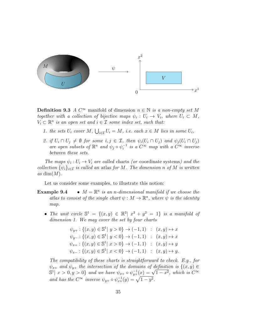
Definition 9.3 A C∞ manifold of dimension n ∈ N is a non-empty set Mtogether with a collection of bijective maps ψi : Ui → Vi, where Ui ⊂ M ,Vi ⊂ Rn is an open set and i ∈ I some index set, such that:

1. the sets Ui cover M ,⋃i∈I Ui = M , i.e. each x ∈M lies in some Ui,

2. if Ui ∩ Uj 6= ∅ for some i, j ∈ I, then ψi(Ui ∩ Uj) and ψj(Ui ∩ Uj)are open subsets of Rn and ψj ψ−1

i is a C∞ map with a C∞ inversebetween these sets.

The maps ψi : Ui → Vi are called charts (or coordinate systems) and thecollection ψii∈I is called an atlas for M . The dimension n of M is writtenas dim(M).

Let us consider some examples, to illustrate this notion:

Example 9.4 • M = Rn is an n-dimensional manifold if we choose theatlas to consist of the single chart ψ : M → Rn, where ψ is the identitymap.

• The unit circle S1 = (x, y) ∈ R2| x2 + y2 = 1 is a manifold ofdimension 1. We may cover the set by four charts

ψy+ : (x, y) ∈ S1| y > 0 → (−1, 1) : (x, y) 7→ x

ψy− : (x, y) ∈ S1| y < 0 → (−1, 1) : (x, y) 7→ x

ψx+ : (x, y) ∈ S1| x > 0 → (−1, 1) : (x, y) 7→ y

ψx− : (x, y) ∈ S1| x < 0 → (−1, 1) : (x, y) 7→ y.

The compatibility of these charts is straightforward to check. E.g., forψx+ and ψy+ the intersection of the domains of definition is (x, y) ∈S1| x > 0, y > 0 and we have ψx+ ψ−1

y+(x) =√

1− x2, which is C∞

and has the C∞ inverse ψy+ ψ−1x+(y) =

√1− y2.

35

• The n-dimensional unit sphere Sn = x ∈ Rn+1|∑n+1

k=1(xk)2 = 1 is amanifold of dimension n. It can be covered by charts in a similar wayas S1, but now 2(n+ 1) charts are needed.

Notice that a general manifold cannot be covered by a single chart.

Exercise 9.5 Show that S2 is a manifold, give the coordinate charts in anal-ogy to S1 and show that the changes of coordinate charts are smooth. (Youmay use symmetries to simplify the problem.)

In addition to specific examples, there are general constructions whichallow us to construct new manifolds from old ones. We mention the mostimportant ones.

First, we call a set O ⊂M an open subset if and only if ψi(O ∩ Ui) is anopen subset of Rn for all charts in the atlas. Any open subset O ⊂ M is amanifold in its own right, where the charts are given by ψi|O : (O ∩ Ui) →ψi(O ∩ Ui) with i ∈ I.

Given two manifolds M and M ′, the product set M ×M ′ is a manifold,where the charts are given by all maps ψi × ψ′j : Ui × U ′j → Vi × Vj, whereψi : Ui → Vi is any chart on M and ψ′i : U ′i → V ′i on M ′. Note thatdim(M ×M ′) = dim(M) + dim(M ′).

Example 9.6

The n-dimensional torus is Tn := S1 × . . .× S1 (n factors). Note that T1 isjust the circle and T2 has the shape of a doughnut.

Exercise 9.7 Sketch T2 as a subset of R3 and sketch a typical product chartobtained from the charts of S1 given in Example 9.4.

A map f : M →M ′ between two manifolds is called k-times continuouslydifferentiable, or Ck, when ψ′i f ψ−1

j is k-times continuously differentiablefor all charts ψj in the atlas for M and all charts ψ′i in the atlas for M ′.As an example we note that, in any chart ψi : Ui → Vi, the coordinatesxk : Rn → R can be used to define smooth maps xk ψi on Ui. Other thansuch local coordinates, we will mostly be concerned with curves, ξ : I →M ,where I ⊂ R is an open interval (which is also a manifold of dimension 1).

All of our manifolds will have some additional properties, which we men-tion here without a very detailed discussion, because they will not be neededexplicitly:

36

1. The atlas of a manifold M is called maximal when it has the followingproperty: Let ψ : U → V be a bijective map between some U ⊂M andan open set V ⊂ Rn and suppose that for all i ∈ I, ψ is compatible withψi in the sense of the second condition in the definition of a manifold.Then ψ is already contained in the atlas ψii∈I , i.e. ψ = ψj for somej ∈ I. Any atlas of a manifold M can always be extended in a uniqueway to a maximal one. We will always assume that our manifolds areequipped with a maximal atlas.

2. All our manifolds are path-connected. This means that for any twopoints p1, p2 ∈ M there is a continuous curve ξ : [0, 1] → M such thatξ(0) = p1 and ξ(1) = p2.

3. All our manifolds are Hausdorff topological spaces. This means thatfor any two points p1, p2 ∈ M there are open sets U1, U2 ⊂ M withpi ∈ Ui, i = 1, 2, but U1 ∩ U2 = ∅. (This is an additional assumptionon M , which we will always make.)

4. All our manifolds are second countable. This means that there is acountable collection Onn∈N of open sets On ⊂ M such that everyopen set O ⊂M contains some On.

All of the examples of manifolds M we have seen so far can be embeddedinto Rm (for some m ≥ dim(M)). However, the importance of manifolds isthat we can investigate them in a framework which is independent of thisembedding. For example, S1 is defined as a subset of R2 and by takingproducts T2 can be viewed as a subset of R4. However, T2 can also beviewed as a subset of R3. Moreover, for the set M that models all eventsin the universe, it is not clear a priori if it can be embedded into any Rm

at all! Also the shape of M is not a priori clear – why should we assumethat it be covered by a single chart like Minkowski space? For these reasons,any information about a manifold should really be formulated in terms ofthe intrinsic structure of the manifold itself, independent of any embedding.We have already done this for the set M and its topological and differentialstructure (i.e. we know what C∞ maps on M are). We now turn to thenotion of tangent vectors.

A C1 curve ξ : I → Rn with 0 ∈ I has a tangent vector at p = ξ(0),which is given by ξµ(0) (where the derivative is taken component-wise in

37

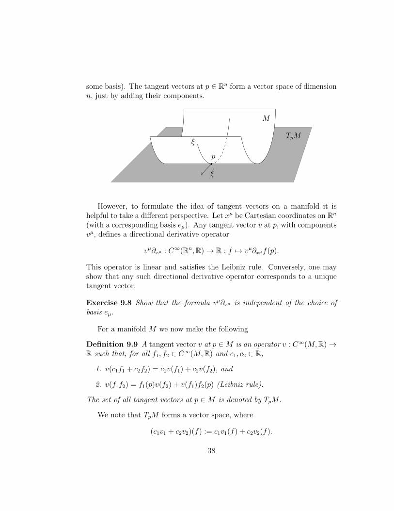
some basis). The tangent vectors at p ∈ Rn form a vector space of dimensionn, just by adding their components.

p

ξ

ξ

M

TpM

However, to formulate the idea of tangent vectors on a manifold it ishelpful to take a different perspective. Let xµ be Cartesian coordinates on Rn

(with a corresponding basis eµ). Any tangent vector v at p, with componentsvµ, defines a directional derivative operator

vµ∂xµ : C∞(Rn,R)→ R : f 7→ vµ∂xµf(p).

This operator is linear and satisfies the Leibniz rule. Conversely, one mayshow that any such directional derivative operator corresponds to a uniquetangent vector.

Exercise 9.8 Show that the formula vµ∂xµ is independent of the choice ofbasis eµ.

For a manifold M we now make the following

Definition 9.9 A tangent vector v at p ∈M is an operator v : C∞(M,R)→R such that, for all f1, f2 ∈ C∞(M,R) and c1, c2 ∈ R,

1. v(c1f1 + c2f2) = c1v(f1) + c2v(f2), and

2. v(f1f2) = f1(p)v(f2) + v(f1)f2(p) (Leibniz rule).

The set of all tangent vectors at p ∈M is denoted by TpM .

We note that TpM forms a vector space, where

(c1v1 + c2v2)(f) := c1v1(f) + c2v2(f).

38

One way to obtain some examples Xµ ∈ TpM is by fixing a chart ψ : U → Vwith p ∈ U and setting

Xµ(f) := ∂xµ(f ψ−1)(ψ(p)),

where the xµ are Cartesian coordinates on Rn. It is not hard to verify thatthe Xµ are indeed in TpM . Moreover, one may show that they form a basisof TpM , so that TpM is a vector space of dimension n = dim(M). (To seethis one first shows that v only depends on the values of f in any (small)neighbourhood of p. One may then use a chart near p to turn the questioninto a problem in ordinary calculus.)

In fact, we may use the chart ψ : U → V to define tangent vectors likeXµ at any point p ∈ U . In this way we obtain a basis for TpM for any p ∈ U ,which is called a coordinate basis. If we use a different chart ψ′ : U ′ → V ′

near p, then the vectors X ′µ are related to the Xµ by the chain rule:

X ′µ =∂xν(x′)

∂x′µXν ,

where xν(x′) is short-hand for xν(ψ ψ′−1(x′)), which describes how the mapψ ψ′ changes the coordinates x′µ into coordinates xν . The quotient can alsobe written in the matrix notation Dν

µ(ψ ψ′−1) (with bases correspondingto the Cartesian coordinates xµ and x′ν).

Similarly, any vector v ∈ TpM can be written as v = vµXµ = v′µX ′µ with

v′µ =∂x′µ(x)

∂xνvν . (15)

This is just the tensor transformation law applied to a vector, except thatthe matrix involved may now depend on the point p ∈M .

Another way to obtain tangent vectors in TpM is to consider a C1 curveξ : I →M with 0 ∈ I and such that ξ(0) = p and setting

D0ξ(f) := ξ0(f) := ∂s(f ξ)(0).

In a chart ψ : U → V with p ∈ U , we can express ξ in terms of its componentsξµ := xµ ψ ξ in Cartesian coordinates xµ:

D0ξ(f) = ∂s(f ψ−1 ψ ξ)(0)

= ∂µ(f ψ−1)(ψ(p)) · ∂sξµ(0)

= ξµ(0)Xµ(f),

39

i.e.

D0ξ = ξµ(0)Xµ.

Many curves can define the same tangent vector in TpM , but every tangentvector in TpM is of this form for some curve ξ.

More generally, let χ : M → M ′ be a smooth map such that χ(p) = p′.Any tangent vector v ∈ TpM gives rise to a tangent vector Dpχ(v) ∈ Tp′M ′

defined by

(Dpχ(v))(f) := v(f χ). (16)

Note that the map Dpχ : TpM → Tp′M′ is linear in v. We recover D0ξ as a

special case, where our notation suppresses the vector v = e1 ∈ T0R, whichis the unit vector which points in the positive direction.

As a general warning we emphasise that for a general manifold thereis no natural way to identify tangent vectors at some point p ∈ M withtangent vectors at some other point q ∈ M . We know that this is possiblein Rn, simply by applying a translation. (More precisely, there is a uniquetranslation τ : Rn → Rn : x 7→ x− (p− q) which maps p to q and Dpτ can beused to identify TpRn with TqRn.) However, such translations are not definedfor general manifolds and there is no natural analog.

9.3 Tangent, Cotangent and Tensor Bundles

In order to systematically keep track of all tangent vectors at all points weintroduce the tangent bundle:

Definition 9.10 The tangent bundle TM of a manifold M of dimension nis the set

TM :=⋃p∈M

p × TpM = (p, v)| p ∈M, v ∈ TpM,

where the union is disjoint (so (p, v) = (p′, v′) if and only if p = p′ andv = v′). We view TM as a manifold of dimension 2n with a maximal atlascontaining all charts of the form

Dψ : TU → V × Rn : (p, v) 7→ (ψ(p), Dpψ(v))

such that v = (Dpψ(v))µXµ in the coordinate basis of TpM determined by ψ.

40

To see that the manifold structure of TM is well defined we notice that forany charts ψ : U → V and ψ′ : U ′ → V ′ with U ∩ U ′ 6= ∅, the change ofcharts from Dψ to Dψ′ is

(Dψ (Dψ′)−1)(ψ′(p), Dpψ′(v)) = (ψ(p), Dpψ(v)),

which is a diffeomorphism. To see this one may write it in component formand use Equation (15) for the vector components.

If χ : M →M ′ is a C∞ map, we may define the tangent map

Dχ : TM → TM ′ : Dχ(p, v) := (χ(p), Dpχ(v)),

where Dpχ was defined in Equation (16).

Definition 9.11 A C∞ vector field is a C∞ map v : M → TM such thatv(p) ∈ Tp(M). The space of all C∞ vector fields is denoted by Γ∞(M,TM).

Because the atlas of TM is closely related to that of M , the smoothnesscondition can be formulated as follows: for any chart ψ : U → V in theatlas of M and the corresponding coordinate bases Xµ of TpM , p ∈ U , thecoefficient functions vµ appearing in

v(p) = vµ(p)Xµ,

must be C∞. This local condition is independent of the choice of chart, so itgives rise to a global condition on v. The simplest example of vector fields,at least on the domain U of a chart ψ, are the coordinate basis vector fieldsXµ.

For any p ∈M , TpM is a vector space, so we may apply the constructionsof Section 9.1. We denote the dual space by T ∗pM and for the space of tensorsof type (k, l) we introduce the notation

T (k,l)p M := TpM ⊗ . . .⊗ TpM︸ ︷︷ ︸

k times

⊗T ∗pM ⊗ . . .⊗ T ∗pM︸ ︷︷ ︸l times

.

We will now show that these linear spaces may be pasted together to formnew manifolds, just like the tangent bundle.

Let us first consider the space T ∗pM , which is called the cotangent spaceof M at p ∈ M . The dimension of T ∗pM equals that of TpM , which isn = dim(M). We may obtain interesting examples of elements in T ∗pM by

41

choosing a function f ∈ C∞(M,R) and defining d pf ∈ T ∗pM by a funnyreversal of perspective in the definition of tangent vectors:

d pf : TpM → R : v 7→ v(f). (17)

d pf is called the differential of f at p ∈M .Using a chart ψ : U → V with p ∈ U we may apply this procedure to the

coordinate functions xµ ψ, which leads to a basis

X∗µ := d (xµ ψ).

At each p ∈ U , this basis is dual to Xµ:

X∗µ(Xν) = Xν(xµ ψ) = ∂xν (x

µ) = δµν .

We therefore call it the dual coordinate basis determined by ψ.Recall that a change of chart at p induces a change of the basis Xµ,

which can be written as a matrix multiplication. The change in the dualbasis is then given by a multiplication with the inverse matrix, as in thetensor transformation law (13).

Definition 9.12 The cotangent bundle T ∗M of a manifold M of dimensionn is the set

T ∗M :=⋃p∈M

p × T ∗pM = (p, ω)| p ∈M, ω ∈ T ∗PM,

where the union is disjoint (so (p, ω) = (p′, ω′) if and only if p = p′ andω = ω′). We view T ∗M as a manifold of dimension 2n with a maximal atlascontaining all charts of the form

D∗ψ : T ∗U → V × Rn : (p, ω) := (ψ(p), D∗pψ(ω))

such that (D∗pψ(ω))µ = ω(Xµ).A C∞ cotangent vector field (or dual vector field or 1-form field) is a

C∞ map ω : M → T ∗M such that v(p) ∈ T ∗p (M). The space of all C∞ dualvector fields is denoted by Γ∞(M,T ∗M).

Note that ω(Xµ) are the components of ω in the dual coordinate basis, ω =ω(Xµ)X∗µ, as may be checked by letting both sides act on the coordinatebasis Xν . The dual coordinate basis X∗µ defines C∞ cotangent vector fields

42

on the domain U of the given chart and a general C∞ cotangent vector fieldcan be expressed as

ω(p) = ωµ(p)X∗µ

with C∞ coefficients ωµ.

General tensors may be treated in an analogous way:

Definition 9.13 The tensor bundle T (k,l)M of type (k, l) on a manifold Mof dimension n is the set

T (k,l)M :=⋃p∈M

T (k,l)p M,

where the union is disjoint. We view T (k,l)M as a manifold of dimensionnk+l+1 with a maximal atlas containing all charts of the form

D(k,l)ψ : T (k,l)U → V × Rnk+l : (p, S) := (ψ(p), (D(k,l)p ψ)S)

such that the components of ((D(k,l)p ψ)S)µ1···µkν1···νl = S(X∗µ1 , . . . , X∗µk , Xν1 , . . . , Xνl).

A C∞ tensor field of type (k, l) is a C∞ map S : M → T (k,l)M such that

S(p) ∈ T (k,l)p (M). The space of all C∞ tensor fields of type (k, l) is denoted

by Γ∞(M,T (k,l)M).

Again the smoothness of a tensor field S means that the components of S inthe basis obtained from Xµ and X∗,ν are smooth functions on M .

A chart ψ : U → V determines a coordinate basis at each p ∈ U forthe tensor bundle. This basis consists of tensor products of Xµ and theirduals X∗,µ. We may express the components of a tensor field T in terms ofthis basis, but we may also use the abstract index notation. Recall that aformula in the abstract index notation is valid when the abstract symbolsare replaced by the components of the tensor in any coordinate basis (cf.Convention 9.2).

The outer product and contraction of tensors can also be defined fortensor fields in a point-wise fashion. Given a tensor field S of type (k, l) anda tensor field T of type (k′, l′), the outer product is a tensor field of type(k + k′, l + l′), given by

(S ⊗ T )a1···ak+k′

b1···bl+l′:= Sa1···akb1···blT

ak+1···ak+k′bl+1···bl+l′

,

43

whereas the contraction over the ith upper index and the jth lower index isgiven by

(CT )a1···ai···akb1···bj ···bl

:= T a1···c···akb1···c···bl .

These equations hold point-wise as identities between linear maps. In ad-dition, given any p ∈ M we may choose a chart ψ : U → V with p ∈ Uand the equations above (in abstract index notation) imply correspondingequalities for the components in the coordinate basis of ψ. These equationsare independent of the choice of the chart ψ, but they only make sense forp ∈ U and not for the entire manifold M . This is an important reason touse abstract indices: because the equations are independent of the choice ofchart and basis Xµ, they make sense on the entire manifold.

Example 9.14 For a vector field va and a dual vector field ωb we can con-struct the (1, 1)-tensor field (v⊗ ω)ab = vaωb and its contraction (Cv⊗ ω) =vaωa. (In this case there is only one choice of indices that we can contract.)The result is a C∞ function on M , which at each point p ∈ M equals thevalue of ω(p) when acting on v(p).

Example 9.15 For any tensor T of type (0, l) we can define a fully anti-symmetric tensor aT by

(aT )b1···bl :=1

l!

∑π∈Sl

ε(π)Tbπ(1)···bπ(l) ,

where Sl is the group of all permutations π of the numbers (1, . . . , l) andε(π) = ±1 according to whether the permutation is odd or even. Such fullyanti-symmetric tensors are called differential forms in the mathematical lit-erature. Note that aT is indeed anti-symmetric in all its indices and thata(aT ) = aT . As a matter of notation we will write

T[b1···bl] := (aT )b1···bl ,

where the square brackets [ ] indicate that the indices should be anti-symmetrisedover.

In a similar way we can also define a fully symmetric tensor sT by

(sT )b1···bl :=1

l!

∑π∈Sl

Tbπ(1)···bπ(l) ,

44

which we will write asT(b1···bl) := (sT )b1···bl .

where the round brackets ( ) indicate that the indices should be symmetrisedover.

With a slight abuse of notation the basis vectors Xµ and their duals X∗µ

are often written as

∂

∂xµ:= Xµ, dxµ := X∗µ.

We have avoided this notation so far, because it suppresses the choice of theψ and treats the tangent vectors ∂

∂xµon V as if they were tangent vectors on

U . (The purpose of the charts ψ is of course to translate the usual differentialcalculus on V into a differential calculus on U , thereby justifying that theabusive notation is indeed valid.)

9.4 Covariant Derivatives

We now turn our attention to derivatives of tensor fields on a manifoldM . Wehave already seen that any C∞ function f : M → R gives rise to a one-formd f defined by d f(v) := v(f). In a chart ψ the one-form locally has the ex-pression (d f)µ = ∂xµf . Under a change of chart, this expression is multipliedby a Jacobi matrix, as usual for a dual vector. For higher order derivatives,however, an expression like ∂xµ∂xνf can be used to define a tensor, but theresulting tensor depends on the choice of coordinates used. In other words,the formula ∂xµ∂xνf is not preserved under changes of coordinates, becausewe also obtain terms involving derivatives of the Jacobi matrix. We nowdiscuss how to eliminate, or at least keep track of, this dependence on thechart, using the notion of (covariant) derivative operators.

Definition 9.16 A (covariant) derivative operator ∇ on a manifold M is amap (or rather a set of maps, for each (k, l))

∇ : Γ∞(M,T (k,l)M)→ Γ∞(M,T (k,l+1)M) : T a1···akb1···bl → ∇b0Ta1···ak

b1···bl

with the following properties:

1. linearity: for all ci ∈ R and tensor fields Ti of type (k, l), ∇(c1T1 +c2T2) = c1∇T1 + c2∇T2, i.e.

∇b0(c1T1 + c2T2)a1···akb1···bl = c1∇b0(T1)a1···akb1···bl + c2∇b0(T2)a1···akb1···bl ,

45

2. Leibniz rule: for all tensor fields T and S, ∇(T ⊗ S) = (∇T ) ⊗ S +T ⊗ (∇S), i.e.

∇b0(Ta1···ak

b1···blSak+1···ak+k′

bl+1···bl+l′) = ∇b0T

a1···akb1···blS

ak+1···ak+k′bl+1···bl+l′

+

T a1···akb1···bl∇b0Sak+1···ak+k′

bl+1···bl+l′

if T is of type (k, l) and T ′ of type (k′, l′).

3. commutativity with contractions: for any tensor field T of type (k, l)with k, l ≥ 1, (∇CT ) = C ′(∇T ), where C contracts the ith upper andjth lower index and C ′ the ith upper and j + 1st lower index:

∇b0(Ta1···c···ak

b1···c···bl) = ∇b0Ta1···c···ak

b1···c···bl ,

4. consistency with differentials: for any C∞ function f , ∇f = d f , i.e.

∇b0f = (d f)b0 .

5. torsion free: for any C∞ function f , ∇∇f is a symmetric tensor, i.e.

∇b0∇b1f = ∇b1∇b0f.

All these properties are familiar from calculus in Rn (except perhaps thecommutativity with contractions). In fact, using a chart ψ : U → V andexpressing tensors in their coordinate basis, one may choose ∇µ := ∂xµ todefine a derivative operator on U . This derivative, however, depends on thechoice of coordinates. That covariant derivatives exist globally will be seenlater, when we prove the existence of a preferred derivative operator.

For a general derivative operator, the action at p ∈M on a general tensorfield T depends only on the values of T in an infinitesimal neighbourhood ofp. This follows form the Leibniz rule and (∇T )(p) = (∇(fT ))(p) when f isa C∞ function with f(p) = 1 and d f(p) = 0. Expanding T in a coordinatebasis, we may use linearity and the Leibniz rule to express ∇T in terms ofderivatives of the basis vector and dual vector fields. Because the derivativeoperator commutes with contractions and its value on functions is known,we also have

ωb∇avb = ∇a(v

bωb)− vb∇aωb.

When ωb ranges over a basis, this allows us to express the action on anyvector field in terms of the action on dual vector fields and functions. Thus,the only freedom we have, is to modify the action on dual vector fields.

46

Theorem 9.17 Given two derivative operators on M , ∇ and ∇′, there is aunique tensor field C of type (1, 2) such that Cc

ab = Ccba and

∇′aωb −∇aωb = Ccabωc (18)

for all dual vector fields ωa. Conversely, given any derivative operator ∇′and a tensor field Cc

ab which is symmetric in its lower indices, Equation(18) defines a derivative operator ∇.

Proof: At any point p ∈ M , ∇aωb − ∇′aωb is a tensor of type (0, 2) whichdepends linearly on ωa. We will show that it actually only depends on thevalues ωa(p) and not on any derivatives. For this purpose we fix any chartψ : U → V with p ∈ U and we define the coordinate functions xµ ψ on U ,µ = 1, . . . , n, where the xµ are Cartesian coordinates on Rn. The local basisX∗µ can be expressed in an abstract index notation as

(X∗µ)a = (d (xµ ψ))a = ∇a(xµ ψ) = ∇′a(xµ ψ)

and we may write (Xµ)c in a similar way. We then view the components ωµ asfunctions on U and write ωa = ωµ(X∗µ)a = ωµ∇a(x

µ ψ) and ωµ = ωc(Xµ)c.Then we compute with Leibniz rule and linearity:

∇′aωb −∇aωb = (∇′aωµ −∇aωµ)(X∗µ)b + ωµ(∇′a∇′b(xµ ψ)−∇a∇b(xµ ψ))

= ωc(Xµ)c(∇′a∇′b(xµ ψ)−∇a∇b(xµ ψ)).

Note that the first term on the right-hand side of the first line vanishes,because all derivative operators have the same action on the functions ωµ.We have now shown that (∇′aωb−∇aωb)(p) is a linear map of ωa(p) withoutany derivatives. This entails the existence of the tensor field Cc

ab. We evenobtain a formula for this tensor field,

Ccab := (Xµ)c(∇′a∇′b(xµ ψ)−∇a∇b(x

µ ψ)),

(which is actually independent of the choice of chart).Conversely, given any derivative operator ∇′ and a tensor field Cc

ab whichis symmetric in its lower indices, one may define

∇b0Ta1···ak

b1···bl := ∇′b0Ta1···ak

b1···bl +k∑i=1

Caib0cT a1···c···akb1···bl

−l∑

j=1

Ccb0bj

T a1···akb1···c···bl .

47

We will omit the straightforward verification that ∇ is indeed a derivativeoperator. 2

In a local chart we may choose ∇′ to be a coordinate derivative. Althoughthis derivative is not covariant, an analog of Theorem 9.17 still works, butnow the components Cρ

µν do not transform like a tensor. In the chosenlocal chart, these components are written as Γρµν and they are called theChristoffel symbol.

Given a covariant derivative operator, it is natural to consider tensorfields whose covariant derivative vanishes. A very useful way of doing this isas follows. Let ξ : I → M be C∞ curve with 0 ∈ I and p := ξ(0) and letva(p) ∈ TpM . Given a covariant derivative operator, we may define uniquevectors va(q) at all points q on ξ such that

ξa∇avb = 0

on the curve. To see why this is true, we choose a chart and write theequation as

0 = ξµ(∂µvν + Γνµρv

ρ) = ∂s(vν ξ) + ξµΓνµρv

ρ.

This is a first order differential equation for the components vνξ as a functionof the parameter s, so given the initial values, it admits a unique solution.The vectors va(q) are called the parallel transports of va(p). Of course asimilar result holds for any tensor. (The general result may be obtained bylinearity and taking tensor products and duals.)

Given a curve ξ : I →M that goes through p, p′ ∈M , we can use paralleltransports to define a map Cξ;p,p′ : TpM → Tp′M . Notice that this mapis linear, because the parallel transport equation is linear. Moreover, it isinvertible, because we can traverse the curve ξ in the opposite direction tofind that Cξ;p′,p is the inverse. This way of identifying tangent spaces atdifferent points is called a connection in the mathematical literature.

As a warning we emphasise that the linear isomorphism Cξ;p,p′ : TpM →Tp′M depends on the choice of the curve ξ.

The fact that connections depend on the choice of a curve ξ is unfamiliarfrom calculus in Rn. Another marked difference between covariant derivativesand ordinary derivatives is the fact that mixed derivatives do not alwayscommute. We do have ∇a∇bf = ∇b∇af for functions f , but for tensors thismay no longer be true. This leads to the concept of curvature.

48

Theorem 9.18 Given a derivative operator ∇ on a manifold M , there is atensor field R d

abc of type (1, 3) such that

∇a∇bωc −∇b∇aωc = R dabc ωd

for all one-form fields ωc.

Proof: The left-hand side is a tensor which depends linearly on ωc. Themain point is to show that the value at any p ∈M depends only on the valueωc(p) and not on any derivatives. For this purpose one may simply work inlocal coordinates and express ∇ in terms of the coordinate derivatives anda Christoffel symbol. A straightforward computation, which we omit, showsthat no derivatives of ω at p appear and

R σµνρ = −∂µΓσνρ + ΓτµρΓ

σντ − (µ↔ ν).

2Using linearity and the Leibniz rule one may show that for general tensors,

(∇a∇b −∇b∇a)Tc1···ck

d1···dl = −k∑i=1

R ciabe T c1···e···ckd1···dl

+l∑

j=1

Re

abdjT c1···ckd1···e···dl .

Definition 9.19 The tensor R dabc is called the Riemann curvature tensor of

∇. The tensor R dadc of type (0, 2) is called the Ricci curvature tensor.

Theorem 9.20 The Riemann curvature tensor has the following properties:

1. R dabc = −R d

bac ,

2. Rd

[abc] = 0,

3. ∇[aRe

bc]d = 0 (Bianchi identity).

Proof: The first property of R dabc is obvious. For the second we note that

∇[µων] = ∂[µων], because the Christoffel symbol is symmetric in its lowerindices. Similarly,

∇[µ∇νωρ] = ∂[µ∂νωρ] = 0

49

by Equation (19) and the fact that ordinary derivatives commute. Thus,

Rσ

[µνρ] ωσ = 2∇[µ∇νωρ] = 0. For the third property we consider

(∇a∇b −∇b∇a)∇cωd = R eabc ∇eωd +R e

abd ∇cωe

and∇a(∇b∇c −∇c∇b)ωd = (∇aR

ebcd )ωe +R e

bcd ∇aωe.

Antisymmetrising over the indices a, b, c, the left-hand sides become equal.Using the properties of the Riemann curvature that we have already shownon the right-hand side leads to

(∇[aRe

bc]d )ωe = Re

[ab|d| ∇c]ωe −R e[bc|d| ∇a]ωe = 0.

As ωe is arbitrary, the Bianchi identity follows. 2

9.5 Metrics and Geodesics

So far we do not have sufficient structure on our manifolds to formulate phys-ically relevant questions: What is the distance between two points? Whatis the shortest path between two points? And is there a preferred choice ofcovariant derivative?

Let us start with the definition of a (pseudo-) metric:

Definition 9.21 A (pseudo-)metric on a manifold M is a smooth tensorfield gab of type (0, 2) such that

1. gab = gba (symmetry),

2. if va ∈ TpM has gab(p)vawb = 0 for all wb ∈ TpM , then va = 0 (non-

degeneracy).

A pair (M, gab) consisting of a manifold with a (pseudo-)metric is called apseudo-Riemannian manifold.

For any va ∈ TM , gabvavb can be viewed as the squared norm of the

vector va. However, gab need not be positive definite, i.e. it need not be truethat gabv

avb ≥ 0 for all va ∈ TM .At any point p ∈ M we can consider the matrix gµν(p) in a coordinate

basis of some chart. This matrix depends on the choice of coordinates, but ithas a number of properties which are independent of this choice. It is always

50

symmetric, so it can be diagonalised and the numbers n+ of positive eigenval-ues and n− = n−n+ of negative eigenvalues are also coordinate independent.In fact, for a given point p ∈M we can always choose coordinates such thatgµν(p) is diagonal with eigenvalues +1 and −1 only. However, this may holdonly hold at the point p! Finally we note that n+ and n− do not depend onthe choice of p, because the components gµν(p) vary smoothly with p and gµνmust remain non-degenerate.

Definition 9.22 The signature of a metric is the pair (n+, n−), where n+ isthe number of positive eigenvalues of the matrix gµν(p) (in a coordinate basisat any point p ∈M), and n− is the number of negative eigenvalues.

We call a metric Riemannian when its signature is (n, 0). In that casewe call the pair (M, gab) a Riemannian manifold.

We call a metric Lorentzian when its signature is (n − 1, 1) and n ≥ 2.In that case we call the pair (M, gab) a Lorentzian manifold, or a spacetime.

For a Riemannian metric, gµν is positive definite. For a Lorentzian metric,gµν is similar to the matrix η of Equation (7).

For a Riemannian manifold (M, gab) and a curve ξ : (a, b) → M we candefine the length of ξ by

ˆ b

a

√gµν(ξ(s))ξµ(s)ξν(s) d s,

i.e. we integrate the length of the tangent vectors along the curve. Note thatthis expression is independent of the choice of parameter.

For Lorentzian manifolds (M, gab) we say that a curve γ : (s1, s2) → Mis spacelike when gab(γ(s))γa(s)γb(s) > 0 for all s. The length of γ is thengiven by

lγ :=

ˆ s2

s1

√gab(γ(s))γa(s)γb(s)d s.

Similarly, γ is called timelike when gab(γ(s))γa(s)γb(s) < 0 for all s. Theproper time of γ is then given by

τγ :=

ˆ s2

s1

√−gab(γ(s))γa(s)γb(s)d s.

For curves which are neither timelike nor spacelike we do not define a lengthor proper time.

51

Because gab is non-degenerate, we can use it to define a bijection

TM → T ∗M : (p, vb) 7→ (p, gab(p)vb),

which is a linear isomorphism from TpM to T ∗pM for each p ∈M . The inverseof this map is a tensor of type (2, 0) and will be denoted by gab, with upperindices, so that

gabgbc = δac

is the identity map on TM . As a matter of notation we will define

va := gab(p)vb, ωa := gab(p)ωb

for any (p, vb) ∈ TM and (p, ωb) ∈ T ∗M . In this way we can use the metric toraise and lower indices, i.e. to identify vectors and dual vectors. The notationcan be extended in an obvious way to all tensors. As a warning, however,we note that in General Relativity, the Lorentzian metric gab is a dynamicalobject, so the identification between vectors and dual vectors is not given apriori. Instead, we must solve Einstein’s equations to find it.

Exercise 9.23 Use the inverse metric gab to show that gabgacgbd = gcd, so the

notation for raising and lowering indices can also be applied in a consistentway to the metric itself.

Suppose that γ : I →M is a curve and va and wb are vector fields alongthe curve which are parallel transports for some covariant derivative operator∇. The inner product gabv

awb along γ changes as follows:

γa∇a(gbcvbwc) = γavbwc∇agbc.

This means that the inner product remains constant if ∇agbc = 0. We nowshow that for a given (pseudo-)metric gab there exists a unique covariantderivative operator which satisfies this additional condition:

Theorem 9.24 Let gab be any (pseudo-) metric on a manifold M . Thenthere exists a unique covariant derivative operator ∇ on M which is compat-ible with gab in the sense that ∇agbc = 0.

Proof: In any chart ψ : U → V we can use the coordinate derivative ∂µ onU . By Theorem 9.17 we can characterise ∇ on U by its Christoffel symbolsΓcab = Cc

ab. We have

0 = ∇µgνρ = ∂µgνρ − Γσµνgσρ − Γσµρgνσ

52

and therefore,

∂µgνρ + ∂νgµρ − ∂ρgµν = (Γρµν + Γνµρ) + (Γρνµ + Γµνρ)− (Γνρµ + Γµρν)

= 2Γρµν ,

where we used the symmetry of the Christoffel symbol. This shows thatany derivative operator which is compatible with gab must have a Christoffelsymbol which is given in any chart by

Γσµν =1

2gσρ(∂µgνρ + ∂νgµρ − ∂ρgµν),

which proves uniqueness of ∇ on U . Conversely, choosing this Christoffelsymbol to define ∇, we also see that ∇ exists on U . We can do this forany chart and on the intersection of any two chart domains, the resultingcovariant derivatives must coincide, because both satisfy the compatibilitycondition. 2

The unique covariant derivative operator which is compatible with gab iscalled the Levi-Civita covariant derivative (or Levi-Civita connection). TheLevi-Civita derivative operator gives rise to a connection Cξ;p,p′ which is notjust a linear isomorphism TpM → Tp′M , but it also preserves inner products,i.e. it maps gab(p) to gab(p

′).We now consider the curvature of the Levi-Civita derivative operator,

starting with some additional notations:

Definition 9.25 The function R := gacRac = gacR babc is called the (Ricci)

scalar curvature of the Levi-Civita derivative. The tensor Gab := Rab− 12Rgab

is called its Einstein tensor.

Theorem 9.26 The curvature of the Levi-Civita derivative operator satisfies

Rabcd = −Rabdc,

Gab = Gba,

∇aGab = 0.

Proof: The first property follows directly from 0 = ∇[a∇b]gcd and Equation

(19). The second property follows from Rd

[abc] = 0, because

Rba = R cbca = −R c

abc −R ccab = −gcdRabcd +R c

acb = Rab.

53

(The first term vanishes by the first property and symmetry reasons.) Forthe third we consider the Bianchi identity ∇[aR

ebc]d = 0 (cf. Theorem 9.20)

and we use the symmetries of the Riemann curvature to compute:

0 = 3gbd∇[aRc

bc]d

= gbd∇aRc

bcd + gbd∇bRc

cad + gbd∇cRc

abd

= ∇agbdRbd −∇dR c

acd −∇cgbdRabcd

= ∇aR− 2∇dRad

= −2∇d(Rad −1

2gadR) = −2∇dGad.

Because the Einstein tensor is symmetric, the result follows. 2

Definition 9.27 A geodesic in a (pseudo-)Riemannian manifold (M, gab) isa curve ξ : I → M whose tangent vectors ξa are parallelly transported alongξ with respect to the Levi-Civita covariant derivative operator.

(Actually, the definition can be made for arbitrary covariant derivative opera-tors on M , but the Levi-Civita derivative operator will be our main interest.)

We think of geodesics as curves which are as straight as possible. Thecondition on the tangent vectors can be written as the geodesic equation:

ξa∇aξb = 0, (19)

or, in a chart and using the parameter s along ξ:

ξµ + Γµνρ(ξ)ξν ξρ = 0.

This is a second order (non-linear) ordinary differential equation for the com-ponents ξµ(s), so its solution is uniquely determined (for s in some maximalinterval) by initial values for ξµ and ξµ. In other words, there exists a uniquemaximal geodesic through any point (p, va) ∈ TM .

Exercise 9.28 Consider Rn as a Riemannian manifold with the constantmetric field gµν = δµν in a global Cartesian chart. Given any tangent vector,(p, vµ) ∈ TRn, show that the unique geodesic ξ with initial data (p, vµ) is

ξµ(s) := pµ + svµ.

54

Exercise 9.29 Show that for any geodesic ξ : I →M , ξaξa is constant alongthe curve ξ.

For spacelike or timelike curves the geodesic equation (19) can be ob-tained from a variational principle. The length lγ, resp. proper time τγ, ofa spacelike, respectively timelike, curve γ between two fixed points attainsa (local) extremum when γ is a geodesic. To verify this one computes theEuler-Lagrange equations of

ˆ √|gab(γ(s))γa(s)γb(s)|d s

to be (in local coordinates (xµ))

0 =−2√

|gµν(ξ)ξµξν |

(−1

2(∂ρgµν)(ξ)ξ

µξν + ∂s(gµρ(ξ)ξµ)

)

and the term in brackets can be rewritten, using ∂s(gµρ(ξ) = (∂νgµρ)ξν and

relabeling indices, as

gµρ

(ξµ + Γµσν ξ

σ ξν).

Example 9.30 (Riemann-tensor and geodesics on S2) The metric of a‘round’ 2-sphere S2 with radius r is by definition

ds2 = r2(dθ2 + sin2 θ dϕ2

)with θ = x1 and ϕ = x2, or in matrix form

(gµν) =

(r2 00 r2 sin2 θ

),

(gµν) =

(1r2

00 1

r2 sin2 θ

).

N

S

ϕθ

55

One can check using the definition of Γσµν that

Γ122 = − sin θ cos θ

Γ212 = Γ2

21 = cot θ

and that all other components vanish.

R 1212 = ∂1Γ1

22 − ∂2Γ112 + Γ1

1αΓα22 − Γ12αΓα12 (sum over α = 1, 2!)

=(sin2 θ − cos2 θ

)− (0) + (0)− (− sin θ cos θ) (cot θ)

= sin2 θ.

To get Rµνσρ with lower indices, we use Rµνσρ = gραRα

µνσ . Then we have

⇒ R2121 = g1αRα

212

= g11R1

212 +g12=0R 2

212

= r2 sin2 θ.

Using the symmetries

R11αβ = R22αβ = Rαβ11 = Rαβ22 = 0

we find R2112 = −R2121,. . . and so on for all 16 components of Rαβγδ.

R11 = gαβR1α1β

= g11R1111

=0 + g22R1212 + 2g12R1121

=0

= 1

R22 = gαβR2α2β

= g11R2121 + g22R2222

=0 + 2g12R2122

=0

= sin2 θ

⇒ R = g11R11 +2g12 =0R12 + g22R22

=2

r2.

It shows, that S2 has a constant scalar curvature.To find the geodesics, let (γµ(t)) = (x1(t), x2(t)) = (θ(t), ϕ(t)). Then we

have the geodesic equation

d2

dt2γµ(t) + Γµαβ (γ(t))

d

dtγα(t)

d

dtγβ(t) = 0

56

Written out using ddt

= ˙ and µ = 1 or µ = 2:

θ − sin θ cos θ (ϕ)2 = 0 and ϕ+ 2 cot θ ϕθ = 0.

One solution is obtained for ϕ = ϕ0 = const. Then we have:

ϕ = ϕ = 0

and we findθ = 0 which implies θ = θ0 + νt.

This describes a segment of a longitudinal great circle of the sphere. Bysymmetry, one can see that all geodesics are great circles.

Example 9.31 Another interesting metric is that of H2, the hyperbolic space(x1 = x, x2 = y > 0) with line element

ds2 =dx2 + dy2

y2,

or in matrix form

(gµν) =

( 1y2

0

0 1y2

)(gµν) =

(y2 00 y2

)(20)

One way to obtain geodesics γ is to go back to the length functional lγ and toremember that geodesics correspond to critical points of this functional. Forpractical computations, let us parameterize the curve by its x-coordinate as

(γµ(x)) = (x, y(x)) which leads to (γµ(x)) = (1, y′(x)) .

(Note that not all curves in H2 can be parameterized that way, but it turnsout that all geodesics which are not vertical lines paralell to the y-axis can.)Then we have

lγ =

ˆdx

√1 + (y′)2

ywhere y = y(x)

and we get the Euler-Lagrange equations(y′

y√

1 + y′2

)′= −

√1 + y′2

y2.

It can be seen that the solutions are arcs of circles in the x-y-plane with thecentre on the x-axis, or vertical lines (exercise).

57

10 General Relativity

We now discuss how the techniques of the theory of manifolds can be used toformulate General Relativity. We will make the following basic assumptions:

1. the set M of all possible events in the universe is a manifold of dimen-sion four,

2. on M there is a Lorentzian metric gab,

3. any pointlike test-object with a mass m > 0 follows a timelike curveξ : I →M ,

4. in the case of free fall, i.e. in the absence of forces other than gravity,ξ is a geodesic.

From now on we will restrict attention to manifolds of dimension four andfor convenience we will also choose physical units such that c = 1.

We have dropped the assumption that M = R4, which is difficult to verifyexperimentally, but we still assume that M locally looks like R4, in the sensethat it is a 4-dimensional manifold. Using this formulation, all charts aretreated on an equal footing and there are no preferred choices of coordinates.In other words coordinates have no intrinsic physical meaning.

We have also replaced the rather rigid structure of ηab, that was of suchfundamental importance in Minkowski space, by a Lorentzian metric gab.This metric may vary from point to point and in some sense we may thinkof it as the gravitational field. It certainly determines the geodesics and thetimelike geodesics are the same for any object, regardless of its mass (weakequivalence principle).

Of course we have yet to supply an equation of motion for the physicalfield gab. Because the gravitational field depends on the mass distributionof the matter in the universe, the equation of motion should also depend onthis matter.

10.1 Kinematics of General Relativity

In this section we will supply some kinematical aspects of General Relativity,describing how observers can measure properties of particles. We will alsoinvestigate how the framework that we have developed so far can implementthe strong equivalence principle, that the outcome of any local experiment in

58

a freely falling laboratory is independent of the initial position and velocityof the laboratory. In addition we will see how the metric gab can encodegravity.

Let us now consider an object, e.g. a particle, following a timelike trajec-tory ξ : I → M in a Lorentzian manifold M . Our first purpose is to definenotions of future and past on M . At each point p ∈ M , the tangent spaceTpM is isomorphic to Minkowski space, so it has two light cones and we canchoose one of these to be the future and the other the past. We can make sucha choice for any p ∈ M , but it is not obvious that we can make this choicein a way that depends smoothly (or continuously) on the base point p ∈M .Such a smooth dependence is desirable in order to avoid pathological situ-ations, where a smooth timelike curve suddenly switches from being futurepointing to past pointing. For this reason we will only consider spacetimeswhich are time-oriented in the following sense:

Definition 10.1 A spacetime (M, gab) is called time-orientable when thereexists a vector field T a on M which is timelike at every point of M . Sucha vector field determines a time-orientation: a timelike vector va ∈ TpM iscalled future pointing if it is in the same light cone as T a (i.e. if vaTa < 0)and past pointing otherwise (vaTa > 0).

A spacetime is called time-oriented if it is time-orientable and a time-orientation has been chosen.

Not every spacetime is time-orientable. However, when a spacetime is time-orientable, then there are many timelike vector fields T a that determine thesame time-orientation. Mathematically speaking, a time-orientation is anequivalence class of timelike vector fields, where two such vector fields T a andT ′a are equivalent if their vectors lie in the same light cone at every point p ∈M . Because M is connected and T a and T ′a are both timelike, it suffices toverify this condition at one point. It follows that a time-orientable Lorentzianmanifold has exactly two time-orientations. We will always assume that achoice of time-orientation can and has been made. Moreover, the trajectoriesof massive objects and observers are always assumed to be future pointing.

We return to our particle, following a timelike, future pointing trajectoryξ : I → M in the Lorentzian manifold M . In analogy to Special Relativitywe can use the proper time along ξ as a parameter:

Theorem 10.2 A time-like curve ξ in a (time-oriented) Lorentzian man-ifold (M, gab) can always be parameterised by proper time, i.e. such thatgab(ξ(τ))ξa(τ)ξb(τ) = −1, without changing its time-orientation.

59

The proof is analogous to that of Theorem 6.5. We may define the velocityand acceleration in terms of the proper time by

va := ξa, aa := ξb∇bξa.

Note that both expressions are independent of any choice of coordinates,whereas the expression ξµ(τ) does depend on this choice. The problem isthat, to quantify the change of va at different values of the proper time τ ,we need to compare tangent vectors at different points of the spacetime M .To do this in a coordinate independent way, we need to use the covariantderivative. Also note that the norm of va is constantly 1, just like in SpecialRelativity. It follows that vaa

a = 0.If the rest mass of the particle is m0, then its energy-momentum and the

force are defined as the dual vectors

Pa := m0va, Fa := vb∇bPa.

Here Fa includes all forces other than gravity. One may easily verify that ifm0 is constant, Fa = 0 is equivalent to the geodesic equation va∇av

b = 0.Let us now consider an observer, who follows another future pointing,

timelike trajectory s 7→ α(s), which we also assume to be parameterised byproper time. The velocity of the observer is αa. If α and ξ both go throughthe point p ∈ M , then the observer may measure properties of the particle.Choosing an inertial frame in TpM and comparing with Special Relativitywe define the energy E and the (spatial) momentum Pa, as measured by theobserver at p, to be

E = −Paαa = −m0ξaαa, Pa = Pa − Eαa.

To obtain Pa we simply projected out the component along αa.The kinematical concepts we introduced above make use of the fact that

for any p ∈ M , the tangent space Tp(M) equipped with the pseudo-innerproduct gab(p) is isomorphic to Minkowski space. We now want to discusshow this identification between TpM and Minkowski space can be made evenmore precise.

Theorem 10.3 (Riemannian normal coordinates) At any p ∈M thereis a diffeomorphism expp of an open neighbourhood W ⊂ TpM containing 0,onto an open neighbourhood U ⊂ M containing p ∈ U , with the followingproperties:

60

1. For any va ∈ W and λ ∈ [0, 1], λva ∈ W ,

2. For any va ∈ W , the curve γ : [0, 1]→M defined by γ(λ) := expp(λva)

is a geodesic with γ(0) = p and γa(0) = va.

The proof uses results on how solutions of differential equations depend ontheir initial data. These can be used to show that the map expp is well-definedand C∞. The fact that it is a diffeomorphism on some neighbourhood W of0 follows from the inverse function theorem.

If we choose an orthonormal basis eµ of TpM , with e0 timelike and with adual basis e∗µ, then we can construct a chart ψ : U → V by setting ψ(x) :=(e∗1(expp(x)), . . . , e∗n(expp(x))). The coordinate system xµ : e∗µ expp hasthe following properties:

xµ(p) = 0, gµν(p) = ηµν , ∂xρgµν(p) = 0.

The last equality is equivalent to the vanishing of the Christoffel symbol atp ∈ M in Riemannian normal coordinates, which follows from the geodesicequation (19) for the curves λ 7→ λxµ. This shows that the identification ofTpM with Minkowski space can even be made up to first order derivatives ofthe metric.

Note that the choice of coordinates heavily depends on the fact thatp ∈ M was fixed in advance, so in this coordinate system these specialproperties typically fail at any other point. However, it is possible to choosecoordinates along any curve such that the metric takes the form gµν = ηµνand the derivatives ∂xρgµν = 0 vanish all along the curve. (Such coordinatesare called Fermi-Walker coordinates.) This explains how General Relativitysatisfies the strong equivalence principle.

One cannot expect to do much better than Fermi-Walker coordinates,because the Riemann curvature tensor R d

abc is independent of the choice ofcoordinates, but its coordinate expression only depends on derivatives of themetric up to second order.

Definition 10.4 A spacetime (M, gab) is called flat, when the Riemann cur-vature tensor vanishes, R d

abc = 0.

One can show that a flat spacetime can be covered by charts on which themetric takes the form ηµν throughout the domain of the chart. I.e., we cancover M by open regions which look like open regions of Minkowski space(including the metric).

61

Our framework very nicely implements the strong equivalence principle,but how exactly does the metric gab encode gravity? The answer to this ques-tion is a bit subtle, because we like to think of gravity as a force which causesacceleration. In General Relativity, however, there is no longer any notionof absolute acceleration, because there is no preferred structure with respectto which something could be accelerated. (This is the ultimate consequenceof treating all charts on an equal footing.) Nevertheless, we can investigatethe relative acceleration of two freely falling objects, which will explain therelation between General Relativity and gravity.

Xa

γ

ξ

Suppose that ξ : (−a, a)→M is a timelike, future pointing geodesic withp := ξ(0) and let Xa ∈ TpM be a vector which is orthogonal to ξa. Wewish to displace p = ξ(0) to an infinitesimally close point in the direction ofXa, track the displaced point as it follows its geodesic and then see how thedisplacement vector changes.

To make these ideas precise we construct a map γ : (−a, a)2 →M as fol-

62

lows (for a suitably small a > 0): We define the geodesic γ(s, 0) := expp(sXa)

and we extend Xa ∈ TpM to the vector field Xa := ∂sγa(s, 0) along the curve.

Note that Xa is parallely transported along the curve, because it is just thetangent vector field of a geodesic.

Next we let T a(γ(s, 0)) be the parallel transport of ξa(0) ∈ TpM alongthe curve γ(s, 0). We then have XaTa = 0 along the curve γ(s, 0), be-cause parallel transports preserve inner products. Finally we define γ(s, t) :=expγ(s,0)(tT

a(γ(s, 0))), i.e. we consider the geodesics generated by the vectorsT a on the curve γ(s, 0). We now extend T a and Xa to the entire range of γby setting T a := ∂tγ

a(s, t) and Xa := ∂sγa(s, t). Note that T a is a tangent

to a geodesic t 7→ γ(s, t), so it is parallelly transported along this geodesic.We have now constructed a one-parameter family of geodesics t 7→ γ(s, t)

with γ(0, t) = ξ(t). We may think of Xa on ξ(t) as the relative position of, orthe infinitesimal displacement to, a nearby geodesic. The relative velocity ofthe nearby geodesic is given by V b := T a∇aX

b and the relative accelerationby

Ac := T a∇a(Tb∇bX

c).

Theorem 10.5 (Geodesic Deviation Equation) In the notations above,

Aa = −R abcd T

bXcT d. (21)

Proof: We first show that T a∇aXb = Xa∇aT

b. This follows from ∂t∂s =∂s∂t as follows. For any smooth function f on M we have X(f) = ∂s(f γ)(s, t) and T (f) = ∂t(f γ)(s, t). The right-hand sides can once again beinterpreted as smooth functions on the range of γ, to which the vectors Xand T can be applied. In this way we find T (X(f)) = ∂t∂s(f γ) = X(T (f)).Using the calculus of covariant derivatives, this means

0 = T a∇a(Xb∇bf)−Xa∇a(T

b∇bf)

= (T a∇aXb)∇bf − (Xa∇aT

b)∇bf + T aXb(∇a∇bf −∇b∇af)

= (T a∇aXb)∇bf − (Xa∇aT

b)∇bf.

Since f was arbitrary, we must have T a∇aXb = Xa∇aT

b.Incidentally, note that T aTa = −1 on the range of γ and hence, by the

geodesic equation for T a,

T a∇a(XbTb) = TbT

a∇a(Xb) = TbX

a∇a(Tb)

=1

2Xa∇a(TbT

b) =−1

2Xa∇a1 = 0.

63

Since XbTb = 0 on γ(s, 0), it follows that XbT

b = 0 on the entire range of γ.

Now we use the geodesic equation for T a and the definition of the Riemanncurvature tensor to compute:

Ac = T a∇a(Tb∇bX

c) = T a∇a(Xb∇bT

c)

= (T a∇aXb)∇bT

c +XbT a∇a∇bTc

= (Xa∇aTb)∇bT

c +XbT a∇b∇aTc −XbT aR c

abd Td

= Xa∇a(Tb∇bT

c)−R cabd T

aXbT d

= −R cabd T

aXbT d.

Relabelling indices yields the result. 2

Equation (21) shows that nearby geodesics can exhibit relative accelera-tion, which is described by the Riemann curvature of the metric. Roughlyspeaking, the gravitational field corresponds to the curvature of the metric.This effect goes under the name gravitational tidal forces.

10.2 Dynamics of General Relativity

In Newton’s theory of gravity, the strength of the gravitational force on atest-mass is determined by the matter in the universe. In General Relativity,gravity is encoded by the metric gab, so it seems reasonable that gab shouldsatisfy an equation of motion, Einstein’s equation, which also involves thematter in the universe. This equation is the topic of the present section.

Because General Relativity should reduce to Newton’s Theory of Gravityin a suitable limit, let us first recall how the dynamics of the latter theory isformulated. For this we revert to classical spacetime, with a classical inertialcoordinate system (t,x), where t is an absolute time coordinate. Let usconsider a continuous distribution of matter, described by a mass density ρ.This mass density gives rise to a gravitational potential Φ, defined by

Φ(x) :=

ˆ−GNρ(x′)

‖x− x′‖d x′,

so that the acceleration that the mass distribution causes on any test-massm is

g(x) = −∇Φ(x) =

ˆ−GNρ(x′)

x− x′

‖x− x′‖3d x′.

64

These are continuous versions of the usual point mass formula for Newton’slaw of gravitation, where the test-mass m drops out, due to the (weak)equivalence principle. Note that ρ can be recovered from Poisson’s equation:

∆Φ(x) = −∇ · g(x) = 4πGNρ(x), (22)

where all derivatives are in the spatial directions. This differential equationtells us how the gravitational potential Φ depends on the mass density dis-tribution ρ. Einstein’s equation should be analogous to Poisson’s equation,but formulated in a relativistic context.

We may compare the acceleration of a test-mass in Newtonian gravity tothe geodesics of General Relativity:

ξi(t) = −∇iΦ(ξ(t)) ←→ ξµ(t) = −Γµνρξν(t)ξρ(t),

where i = 1, 2, 3 and µ = 0, 1, 2, 3. Now suppose that we can choose coor-dinates xµ such that x0 is a time coordinate in which the variations of themetric are negligible, i.e. the gravitational field is constant. Also supposethat the velocity of the test-mass is small, so that ξρ(t) is close to (1, 0, 0, 0).The comparison above then suggests that

∇iΦ ←→ Γi00 = −1

2giµ∂µg00

and Φ might correspond to Φ ' −12− 1

2g00. (The term −1

2is needed to find

the Minkowski metric component g00 = −1 in the absence of masses.)To find a suitable correspondence for ∆Φ we need to consider second

order derivatives. For this purpose we will investigate the gravitational tidalforces from the point of view of Newton’s Theory of Gravitation. GivenΦ(x) we can consider two freely falling particles at time t, at positions x andx + h. Their respective accelerations will be −∇Φ(x) and −∇Φ(x + h), sothe relative acceleration is

−∇Φ(x + h) +∇Φ(x).

To find the relative acceleration of a particle which is infinitesimally close tothe particle at x we take the derivative with respect to h at h = 0 in thedirection X, which yields

−(X · ∇)∇Φ(x).

65

This is the gravitational tidal force in the setting of Newtonian gravity andshould be compared with the result in General Relativity, Theorem 10.5:

−R abcd T

bT d ←→ −∇c∇aΦ.

Here the timelike vector T b can be compared to the classical flow of absolutetime and, due to the antisymmetry properties of the Riemann curvature ten-sor, the indices a and b only range over the spatial coordinates. Contractingover a and b yields a suitable analogue of the term 2Φ in Poisson’s equation:

RbdTbT d ←→ ∆Φ. (23)

Now we turn to a relativistic formulation of the mass density ρ. Keepingin mind the lesson of Special Relativity that mass is energy, it makes senseto compare ρ with an energy density. For a continuous (or C∞) distributionof matter in a spacetime M , we define the energy density at a point p ∈M ,from the perspective of an observer at p ∈ M , to be the quotient of themass in a spatial region B divided by the volume of B, in the limit where Bshrinks to the point p. To see what this limit entails we consider an example,consisting of a matter distribution in Minkowski space, which we assume toconsist of particles which are all at rest in some inertial frame. Now considertwo inertial observers, related by a Lorentz boost, but both going throughthe same point p ∈M with velocity vectors T a and T ′b, respectively. Supposethat the first observer is also at rest, so he measures an energy density whichconsists entirely of the rest masses of the particles, leading to a mass densityρ, say. To compute the result for the second observer, we apply a Lorentztransformation. We recall the following two relevant effects: the rest massesget multiplied by a factor γ = TaT

′a and the lengths in the direction ofmotion get multiplied by a factor γ−1. The energy density for the secondobserver therefore becomes ρ′ = γ2ρ. The results so far can be formulatedvery neatly as follows:

ρ′ = TabT′aT ′b, Tab := ρTaTb.

Generalising this idea leads to the following:

Tenet 10.6 A continuous matter distribution in a spacetime (M, gab) canbe described by a symmetric tensor Tab = Tba, the stress-energy-momentumtensor (which we will often abbreviate to stress tensor, for convenience). Foran observer with velocity T a ∈ TpM , the components of Tab are interpretedas follows:

66

1. TabTaT b is the energy density at p,

2. TabvaT b is the momentum in the direction va, if vaT

a = 0,

3. Tabvawb is the (va, wb)-component of the stress tensor, if vaT

a = 0 andwaT

a = 0.

For normal matter, the stress tensor is conserved, ∇aTab = 0, and itsatisfies the weak energy condition: TabT

aT b ≥ 0 for all timelike vectors T a.

In Special Relativity, the conservation equation∇aTab = 0 is equivalent to theconservation of energy-momentum. In General Relativity, this interpretationonly holds when gravity does not exert forces on the matter.

Thus, given a timelike vector T a and a stress tensor Tab we choose thequantity TabT

aT b to correspond with the mass density ρ for the observerdescribed by T a. In order to obtaine the appropriate analogue of Poisson’sequation in General Relativity, we note that we may also choose instead thecorrespondence

2

(Tab −

1

2gabT

cc

)T aT b ←→ ρ. (24)

To see this, we note that the main contribution to T cc comes from the energydensity TabT

aT b, because the stress components in the stress tensor are typi-cally comparably small in units where c = 1. The values of the left-hand sideis therefore very close to TabT

aT b, so the correspondence is still physicallyreasonable.

Together with the correspondence in Equation (23) we may now rewritePoisson’s equation as RabT

aT b = 8πGN

(Tab − 1

2gabT

cc

)T aT b. Assuming that

this holds for all timelike vectors T a leads to

Rab = 8πGN

(Tab −

1

2gabT

cc

).

In order to obtain an equation which just contains Tab on the right-handside we proceed as follows. Contracting over the indices a and b we findR = −8πGNT

cc. This can be used to eliminate the term T cc in favour of

R, which can be brought to the other side of the equation. The result isEinstein’s equation:

Gab = Rab −1

2gabR = 8πGNTab. (25)

67

Einstein’s equation is a non-linear partial differential equation for thecomponents of the metric gab, which occur in Einstein’s tensor Gab withderivatives up to second order. The metric also occurs in the equations ofmotion of any matter in the universe, which, in turn, determine the form ofTab. One ought to solve all these equations of motion together.

From Bianchi’s identity, ∇aGab = 0 (cf. Theorem 9.20) we immediatelyfind ∇aTab = 0. This equation already imposes a strong, but physically jus-tifiable restriction on the matter in the universe. Note that if we had chosenthe correspondence TabT

aT b = ρ in our derivation of Einstein’s equation, wewould instead have found Rab = 8πGNTab which would not have been con-sistent with the conservation of the stress tensor. In many cases, ∇aTab = 0encodes the full equations of motion of this matter.

It is possible to formulate Einstein’s equation as a Cauchy problem. Thismeans that one can prescribe a manifold Σ of dimension 3 and initial valuesfor the metric gab and its “normal” derivatives on Σ and then construct aunique, maximal manifold M with a Lorentzian metric gab which contains Σas a spacelike hypersurface and whose metric has the correct data on Σ. Wewill not consider the rather technical aspects of this formulation.

10.3 Properties of General Relativity

With Einstein’s equation in place, the content of General Relativity can beformulated concisely as follows (cf. [8]):

Tenet 10.7 (General Relativity) Spacetime is a four-dimensional man-ifold with a Lorentzian metric, whose relation to the matter distribution inspacetime is given by Einstein’s equation (25).

Before we proceed to discuss a number of physical predictions and ap-plications of this theory, let us pause to mention a few general properties ofit.

If the Lorentzian manifold (M, gab) is a solution to Einstein’s equation forsome stress tensor Tab, then we can immediately construct further solutionsusing embeddings:

Definition 10.8 An embedding of manifolds M,M ′ of the same dimension,is a smooth injective map ψ : M → M ′ such that the range ψ(M) ⊂ M ′ isopen and the map ψ−1 : ψ(M)→M is also smooth.

68

A diffeomorphism is a surjective embedding ψ : M →M . Because the in-verse ψ−1 : M →M is also a diffeomorphism, the set of all diffeomorphismsof a manifold M forms a group.

One particular kind of embedding is the canonical inclusion map U → Mof a subset U ⊂ M . Another kind is the charts that were used to definemanifolds in the first place.

Given any embedding ψ : M → M ′, we can use ψ and ψ−1 to maptangent vectors and tensors from a point p ∈ M to a point ψ(p) ∈ M ′ andback. Assuming that all laws of physics can be formulated in terms of tensorfields (or similar geometric objects), we can use ψ and ψ−1 to transport allfields from M ′ to M , just as we did for charts. Now suppose that M ′ hasa Lorentzian metric g′ab and various tensor fields collectively denoted by φ,and let use denote by gab := ψ∗g′ab respectively φ = ψ∗φ′ the metric andtensor fields that we obtain on M via the embedding ψ. If (g′ab, φ

′) satisfiesEinstein’s equation on M ′, then so does (gab, φ) on M . In formulae, if wewrite Einstein’s equation as Eab(g, φ) = 0 (Eab being the left minus rightside), then Eab is such that

Eab(g, φ) = ψ∗Eab(g′, φ′)

for any embedding ψ : M →M ′ and (gab, φ) related to (g′ab, φ) in the mannerdescribed above. The above property of the Einstein field equations is of-ten referred to as general covariance. One can show that general covarianceimplies, under certain reasonable technical assumptions, that Eab must be alocal differential operator, i.e. Eab|p can be written, at each p as a contractionof (gab, g

ab, φ, . . . ,∇(a1 . . .∇ar)φ,Rabcd, . . . ,∇(a1 . . .∇as)Rabcd)|p, where the or-ders r, s are locally bounded (Peetre’s theorem, Thomas replacement theo-rem). Of course, we want Eab to be given by the Einstein field equationwith a local matter stress tensor, so general covariance along does not implyEinstein’s equation but would hold for a broad class of field equations.

Intuitively speaking, general covariance means that the laws of physicscannot contain any non-dynamical quantities that refer to spacetime otherthan the metric gab (and possibly the time-orientation and orientation ofM), and any other dynamical fields φ on a manifold M , and that the lawsare described by partial differential equations (Einstein field equation). Anexample of a non-dynamical quantity would be a preferred coordinate system,which we can think of as a collection of four scalar fields x0, . . . , x3 : M → Rsuch that (∇ax

0, . . . ,∇ax3)|p spans T ∗pM at each point p. Of course, there

69

is no difficulty having a dynamical coordinate system. In this case, our fourscalar fields would have to enter the stress tensor Tab in a generally covariantway. Such theories are sometimes called “Einstein-ether”-theories, becausethe four scalar fields locally define a frame. From a general perspective, thereis nothing special about such theories compared to theories with other kindsof matter fields.

Another consequence of general covariance is that the individual pointsp ∈ M have no intrinsic physical meaning. In fact, we can only identify apoint p by giving it a physical description, e.g. that it is the point where cer-tain physical fields (including the metric gab) take certain prescribed values.Now, if we apply a diffeomorphism ψ to the Lorentzian manifold (M, gab) toobtain the new field configurations (M,ψ∗g′ab), then a point p ∈ M remainsfixed, but the field configurations do not, so the physical description will nowdetermine the point ψ(p), rather than p.

Apart from being generally covariant in the above sense, which, as wehave seen, is a feature of a broad class of theories, Einstein’s equation arealso local in another, more subtle sense. This property has to do with the factthat the Einstein field equations are basically hyperbolic partial differentialequations. The prototype of such a hyperbolic equation is the wave equationfor a scalar field φ : M → R on a fixed spacetime (M, gab),

∇a∇aφ = j .

Suppose (M, gab) does not have any grossly pathological causal features, inthe sense that there is a space like embedded hyper surface Σ ⊂ M withthe property that every inextendible causal curve γ : (a, b) → M (meaningγa timeline or null everywhere) intersects Σ precisely once. Then it can beshown that the wave equation has a well-posed initial value problem: For eachj ∈ C∞0 (M), and each choice of p, q ∈ C∞0 (Σ), there is a smooth solution φhaving φ|Σ = q, na∇aφ|Σ = p, where na is the unit normal to Σ. Furthermore,if we change j in the causal future of Σ, then φ does not change in the causalpast of Σ. Likewise, if we change p, q inside some compact set K ⊂ Σ, thenφ does not change outside the domain of causal influence of K, i.e. outsidethe set of points p that can be connected to K by a causal curve. Sincethere are many ways of choosing Σ, j, p, q, this implies a kind of locality (i.e.local dependence on the source and initial conditions). There is a sense inwhich Einstein’s equations are also hyperbolic and possess an initial valueformulation of the above kind, although this feature is complicated by the fact

70

that Einstein’s equations are also generally covariant. A detailed discussionis outside the scope of our lectures and can be found e.g. in [?]. Let us onlymention here that this feature is tightly related to the special form of Eaband is not shared by most other generally covariant field equations.

10.4 Stress-Tensor and Energy Conditions

Let us list some stress tensors for various matter models.

1. Incoherent matter (a.k.a. dust): pointlike particles that follow timelikepaths without influencing each other. The flow of the particles can bedescribed by a future pointing, timelike velocity vector field ua withuaua = 1 with ua∇au

b = 0 (so each particle follows a geodesic). Thestress tensor is

Tab = ρuaub,

where ρ : M → R>0 is a positive mass density function that satisfiesthe continuity condition ∇a(ρu

a) = 0.

2. Perfect fluids: analogous to dust, but now the particles exert a pressureP on each other, P : M → R. Using the same notations as before, thevector field ua may no longer have geodesics as its integral curves. Thestress tensor is

Tab = ρuaub + P (uaub + gab).

Note that the weak energy condition is satisfied, because γ := uaαa ≥ 1

and hence (ρ+P )γ2−P ≥ ρ ≥ 0. The conservation∇aTab does give riseto conditions on ρ, P and ua, which may be interpreted in terms of fluiddynamics. (In the non-relativistic limit, they reduce to conservation ofmass and Euler’s equation).

3. Electromagnetic fields: In Special Relativity, an electromagnetic fieldis described by a one-form Aa, modulo a gauge equivalence relation,Aa ∼ 0 iff Aa = ∇aλ for some function λ. From Aa one constructsa field-strength tensor Fab := 2∇[aAb], which is antisymmetric. Its sixindependent components encode the electric and magnetic fields, which,however, are observer dependent. Let eµ ∈ TpM be an orthonormalframe and consider an observer at p ∈M with velocity vector e0 (which

71

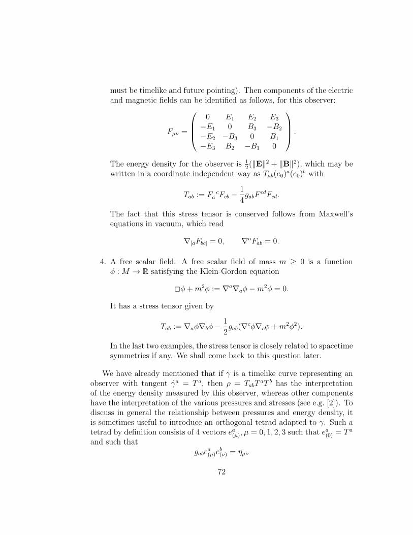
must be timelike and future pointing). Then components of the electricand magnetic fields can be identified as follows, for this observer:

Fµν =

0 E1 E2 E3

−E1 0 B3 −B2

−E2 −B3 0 B1

−E3 B2 −B1 0

.

The energy density for the observer is 12(‖E‖2 + ‖B‖2), which may be

written in a coordinate independent way as Tab(e0)a(e0)b with

Tab := F ca Fcb −

1

4gabF

cdFcd.

The fact that this stress tensor is conserved follows from Maxwell’sequations in vacuum, which read

∇[aFbc] = 0, ∇aFab = 0.

4. A free scalar field: A free scalar field of mass m ≥ 0 is a functionφ : M → R satisfying the Klein-Gordon equation

2φ+m2φ := ∇a∇aφ−m2φ = 0.

It has a stress tensor given by

Tab := ∇aφ∇bφ−1

2gab(∇cφ∇cφ+m2φ2).

In the last two examples, the stress tensor is closely related to spacetimesymmetries if any. We shall come back to this question later.

We have already mentioned that if γ is a timelike curve representing anobserver with tangent γa = T a, then ρ = TabT

aT b has the interpretationof the energy density measured by this observer, whereas other componentshave the interpretation of the various pressures and stresses (see e.g. [2]). Todiscuss in general the relationship between pressures and energy density, itis sometimes useful to introduce an orthogonal tetrad adapted to γ. Such atetrad by definition consists of 4 vectors ea(µ), µ = 0, 1, 2, 3 such that ea(0) = T a

and such thatgabe

a(µ)e

b(ν) = ηµν

72

where ηµν = diag(−1, 1, 1, 1) is the Minkowski metric. With this notation

Tabea(0)e

b(0) = ρ = energy density

Tabea(0)e

b(i) = Pi = momentum density

Tabea(i)e

b(j) = θij = stresses

in the “orthogonal frame” defined by the tetrad. Different tetrads definingthe same space- and time orientations are related by a proper orthochronousLorentz transformation, e′a(µ) = Λµ

νea(ν), and these change the energy density,pressure density, and stress density in the usual way familiar from SpecialRelativity.

Energy conditions specify in general terms properties expected to holdfrom physical considerations. These conditions are traditionally groupedinto the following categories.

a. Weak energy condition (WEC): For all timelike or null T a we have

TabTaT b ≥ 0.

For a perfect fluid with stress tensor Tab = ρuaub + Phab and fluidvelocity ua, this means that ρ+ P ≥ 0 and ρ ≥ 0.

b. Null energy condition (NEC): We have

Tablalb ≥ 0

for all null la. For a perfect fluid, it means ρ + P ≥ 0. Note that theweak energy condition leads to the null energy condition.

c. Dominant energy condition (DEC): For all timelike T a, the conditionrequires that the vector

f b = −T baT a

is a timelike or null future pointing vector. Note that the dominantenergy condition leads to the weak energy condition. The dominantenergy condition and Einstein’s equation lead to the positive mass the-orem. For a perfect fluid, it means that ρ ≥ |P |.

73

d. Strong energy condition (SEC): For all timelike T a, this condition re-quires that

TabTaT b ≥ 1

2T ccT

aTa.

Note that the strong energy condition implies the null energy conditionbut it does not imply the weak energy condition. The strong energycondition and Einstein’s equation leads to focussing of geodesics (seeRaychaudhuri equation).

It is instructive to illustrate the meaning of the various energy conditionsfor a perfect fluid with stress tensor Tab = ρuaub + Phab.

74

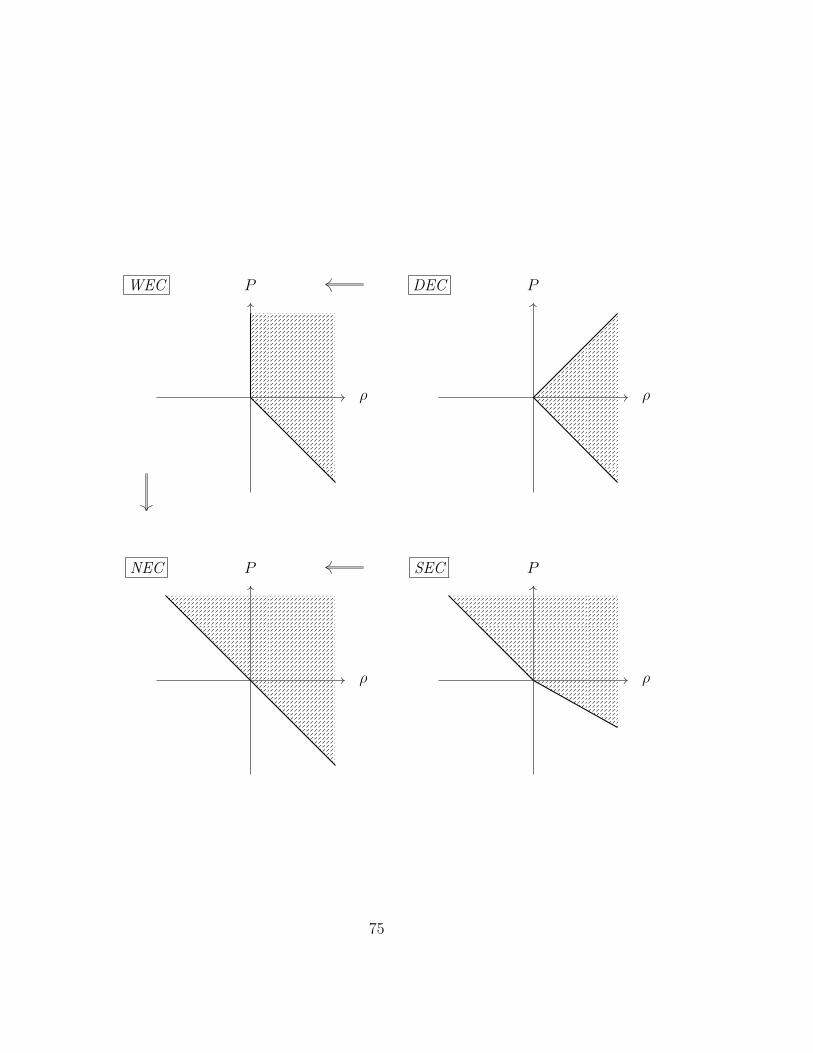
ρ

P

ρ

P

ρ

P

ρ

P

WEC DEC

NEC SEC

75

Part III

Applications of GeneralRelativityThe conceptual changes and theoretical improvements of Einstein’s GeneralRelativity are by no means purely academic. Many subtle consequences ofhis theory have been experimentally verified during the past century andthe theory now forms the basis of our understanding of the universe at largescales (cosmology), introducing the notion of a big bang and of black holes atthe centres of galaxies. Closer to home, General Relativity is needed for theproper working of the Global Positioning System (GPS), because the older,less precise descriptions of radio signals in the Earth’s gravitational field leadto errors of many meters. The most direct prediction of General Relativity,however, is that gravity is a field theory, so it propagates in the form of waves,rather than acting at a distance. A direct observation of these gravitationalwaves is difficult, because their effects are very small, but at present severalexperiments are underway and it is hoped that the first gravitational waveswill soon be observed, leading to novel ways to look up into the sky andstudy the universe we live in.

11 Spacetime Symmetries

As in other branches of theoretical physics, in order to understand the im-plications of Einstein’s equation, we have to study solutions describing realphysical situations. Given the complexity of the equations, one must either

1. find solutions by numerical methods, or

2. make stringent symmetry assumptions and try to find analytic solu-tions.

The numerical analysis of Einstein’s equations is a very important areaof General Relativity, which is, however, beyond the scope of these notes.We therefore focus on the second option. It is surprising that solutionsrepresenting the two most important physical phenomena predicted by thetheory can be found in this way:

76

1. cosmological solutions (Friedmann-Lemaıtre-Robertson-Walker metric)describing a dynamical cosmos,

2. black hole solutions (Schwarzschild, Kerr metric) describing objectsfrom which no light can escape.

Before we come to these, it is useful and necessary to understand the natureof symmetries in General Relativity.

Since we describe spacetime geometry by a pair (M, gab) consisting of amanifold M and a Lorentzian metric gab, a symmetry is a map ψ preservingthis structure. Thus, first of all ψ should be a diffeomorphism of M . In orderto formulate that ψ preserves gab, we need the notions of pull-back and push-forward of tensors. The notion of push-forward is defined as follows. Let va

be a vector at p ∈ M . Choose a curve γ(s) in M whose derivative γa(0)equals va. The push forward of va, denoted ψ∗v

a, is the vector at ψ(p) whichis equal to the derivative (d/dt)(ψ γ)(0). The notion of pull-back applies toco-vectors and is defined by duality. Let wa be a covector at ψ(p). The pullback, denoted ψ∗wa is the covector at p whose action on va is related by

(ψ∗wa)va

∣∣∣∣p

= waψ∗va

∣∣∣∣ψ(p)

.

The notions of pull-back and push forward apply straightforwardly to tensorsof higher rank. Coordinate expressions for the push-forward and pull-backare obtained as follows. Near p and ψ(p) pick local coordinates xµ and x′µ.Let us write ψ(x)µ = x′µ for the action of ψ in these local coordinates. (Notethat there is slight abuse of notation here because ψ is really a map fromM to M and not between coordinate vectors. What is meant here is thecomposition of ψ with the coordinate charts at p and ψ(p)). Then, if tab...c isa tensor field with coordinate components tµν···σ, the pull-back has coordinatecomponents

(ψ?t)µν···σ (x) = tαβ···γ(x′)∂x′α

∂xµ· · · ∂x

′γ

∂xσ(26)

where (x′µ) is viewed as a function of (xµ) in local coordinates (note thesimilarity with the transformation law for covariant tensors which of courseis not accidental).

Definition 11.1 A diffeomorphism ψ on M is called an isometry (or “sym-metry”) if ψ∗gab = gab.

77

The isometries of a spacetime (M, gab) always form a Lie group becauseone can easily show that both the composition, as well as the inverse, ofisometries are again isometries, and because these operations are continuousin a natural sense.

Example 11.2 (Minkowski space) In the case M = R4, gab = ηab, theisometries consist precisely of translations and Lorentz-transformations. Thegroup of all isometries is isomorphic to O(3, 1) nR4, the Poincare group.

Just as the spacetime symmetries (isometries) form a Lie group, infinites-imal symmetries are associated with the Lie algebra of this group. Geomet-rically, infinitesimal symmetries are represented by vector fields ξa on Mwhich, intuitively, describe “infinitesimal displacements”. This can be madeprecise as follows. We call ψtt∈R a 1-parameter group of diffeomorphismsif ψt ψs = ψt+s for all s, t ∈ R and if ψt=0 = idM = identity on M . Given a1-parameter group of diffeomorphisms, we can define a corresponding vectorfield ξa by the condition that

∂

∂tf(ψt(x))

∣∣∣t=0

= ξa(x)∇af(x) (27)

holds for all smooth real valued functions f on M . Given a covariant tensorfield tab...c on M , we call the operation

(Lξt)ab...c :=∂

∂t(ψ?t t)ab...c

∣∣∣t=0

the Lie-derivative. The Lie derivative is independent of any choice of covari-ant derivative operator, but if we are given any covariant derivative operator,we may express the Lie derivative in terms of it:

(Lξt)ab...c = ξd∇dtab···c − (∇aξd)tdb···c − (∇bξ

d)tad···c · · · − (∇cξd)tab···d

In particular, we may choose ∇a = ∂a to be the flat derivative operatorassociated with some local coordinate system. This give a practical way tocalculate the Lie derivative in coordinates, and to verify this formula usingthe coordinate expression for the pull-back, see (26).

Exercise 11.3 Check that the right side is indeed independent of the choiceof covariant derivative operator.

78

Definition 11.4 A vector field on M is called “Killing” for a spacetime met-ric gab on M if (Lξg)ab = 0. (Using the above expression for the Lie-derivativewith ∇a equal to the Levi Civita connection for gab, this is equivalent to

∇aξb +∇bξa = 0 (for ξa = gabξb)

since ∇agbc = 0.)

The relationship between Killing vectors and symmetries is the following.If ψtt∈R is a 1-parameter group of symmetries of gab, then by definition,Lξgab = 0. Conversely, if ξa is a Killing vector field, then there exist a 1-parameter group of symmetries ψtt∈R such that (28) holds. Just as theisometries of a spacetime form a Lie group, the infinitesmial symmetries(Killing vector fields) form a Lie algebra whose commutator is given by thecommutator of vector fields (see exercises).

Example 11.5 For the symmetries in Example 11.2 we have:

1. For the translations in the z-direction, the associated infinitesmal gen-erator (Killing vector field) is (ξµ) = (0, 0, 0, 1) in inertial coordinates(xµ) = (t, x, y, z).

2. For rotations around the z-axis, (ξµ) = (0, 0,−z, y), and

3. for boosts along the x-axis, (ξµ) = (x, t, 0, 0).

12 Cosmological Solutions to Einstein’s Equa-

tion (Maximally Symmetric Universes)

Maximally symmetric universes are among the simplest, yet most importantsolutions to Einstein’s equations. The form of their metric is restricted, upto one free function of time, by symmetry assumptions, whereas this functionis determined by Einstein’s equations. Let us first discuss the symmetries.We assume that M = R× Σ, and we assume that the line element is of thegeneral form

ds2 = −dt2 + a(t)2γij(x)dxidxj

where i, j = 1, 2, 3 are coordinates on Σ. It is furthermore assumed that,for each fixed t, γijdx

idxj gives Σ the structure of a homogeneous, isotropicRiemannian manifold. Such a manifold by definition satisfies the followingconditions:

79

1. Isotropy: For each p ∈ Σ and any pair of unit vectors vi, wj at pthere exists an isometry ψ of (Σ, γij) such that (ψ?v)j = wj. For eachorientation of Σ, there exists an isometry reversing the orientation.

2. Homogeneity: For each p, p′ ∈ Σ there exists an isometry ψ such thatψ(p) = p′.

The factor a(t) > 0 is called the scale factor. It is essentially the only non-trivial ingredient in the line element because it turns out that (Σ, γij) mustbe maximally symmetric Riemannian spaces whose metric is basically fixed(locally) once we specify the (necessarily constant) curvature of (Σ, γij). Inorder to see that (Σ, γij) is basically “just symmetry”, consider any fixedpoint p ∈ Σ, and let G be the isometry group. We may then define the“isotropy subgroup” G0 leaving this point invariant. Any isometry ψ ∈ G0

induces the linear isometric map vj 7→ ψ∗vj in the tangent space TpΣ. Thus,

G0 is a subgroup of the group of linear isometric transformations of TpΣ(relative to the metric γij|p), and hence isomorphic to a subgroup of O(n)(in n spatial dimensions). However, G0 must actually be equal to O(n). Otherwise, we could construct an invariant vector vi (under G0), or aninvariant orientation. This is forbidden by our requirement of isotropy. Ifp′ is any other point in Σ, there is an element ψ ∈ G which carries p top′ by the homogeneity assumtion, and this element must be unique up toψ 7→ ψ ψ′, where ψ′ ∈ G0. Hence, we can put points in Σ into one-to-onecorrespondence with elements of G modulo elements of G0

∼= O(n) (actingby right multiplication on G). In other words, Σ must be a quotient G/O(n)of dimension n. It is then possible to see that the only possibilities for Gcan be G = O(n + 1), E(n), O(n, 1), i.e. Σ is a maximally symmetric space.Furthermore, using this information, one can derive the local form of γijusing methods from Lie group theory.

Here, we will derive the local form γij by a different, more explicit “byhand” method. One can show that a maximally symmetric space of dimen-sion n necessarily has ([5]) a Riemann tensor of the form

Rijkl = k (γikγjl − γilγjk),

where k in the last line is a real constant, and Rijkl is the Riemann tensorof γij (not to be confused with the ijkl-component of the Riemann tensorof the full spacetime metric!) 6. In n = 3 spatial dimensions, the case of

6As an aside, we note that this condition can also be stated as DiRjklm = 0, where Di

is the Levi-Civita connection of γij

80

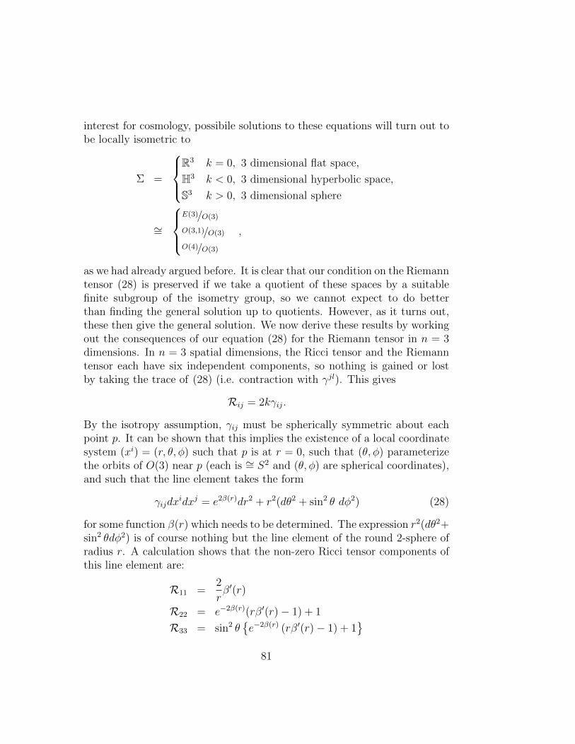
interest for cosmology, possibile solutions to these equations will turn out tobe locally isometric to

Σ =

R3 k = 0, 3 dimensional flat space,

H3 k < 0, 3 dimensional hyperbolic space,

S3 k > 0, 3 dimensional sphere

∼=

E(3)/O(3)

O(3,1)/O(3)

O(4)/O(3)

,

as we had already argued before. It is clear that our condition on the Riemanntensor (28) is preserved if we take a quotient of these spaces by a suitablefinite subgroup of the isometry group, so we cannot expect to do betterthan finding the general solution up to quotients. However, as it turns out,these then give the general solution. We now derive these results by workingout the consequences of our equation (28) for the Riemann tensor in n = 3dimensions. In n = 3 spatial dimensions, the Ricci tensor and the Riemanntensor each have six independent components, so nothing is gained or lostby taking the trace of (28) (i.e. contraction with γjl). This gives

Rij = 2kγij.

By the isotropy assumption, γij must be spherically symmetric about eachpoint p. It can be shown that this implies the existence of a local coordinatesystem (xi) = (r, θ, φ) such that p is at r = 0, such that (θ, φ) parameterizethe orbits of O(3) near p (each is ∼= S2 and (θ, φ) are spherical coordinates),and such that the line element takes the form

γijdxidxj = e2β(r)dr2 + r2(dθ2 + sin2 θ dφ2) (28)

for some function β(r) which needs to be determined. The expression r2(dθ2+sin2 θdφ2) is of course nothing but the line element of the round 2-sphere ofradius r. A calculation shows that the non-zero Ricci tensor components ofthis line element are:

R11 =2

rβ′(r)

R22 = e−2β(r)(rβ′(r)− 1) + 1

R33 = sin2 θe−2β(r) (rβ′(r)− 1) + 1

81

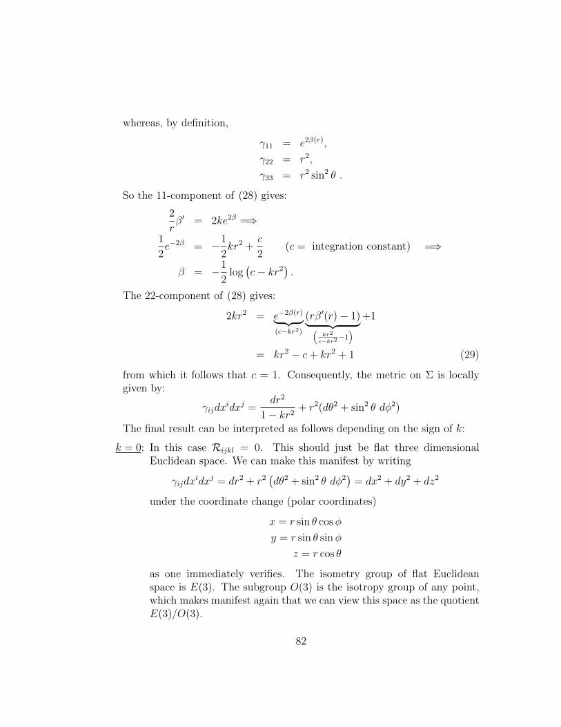
whereas, by definition,

γ11 = e2β(r),

γ22 = r2,

γ33 = r2 sin2 θ .

So the 11-component of (28) gives:

2

rβ′ = 2ke2β =⇒

1

2e−2β = −1

2kr2 +

c

2(c = integration constant) =⇒

β = −1

2log(c− kr2

).

The 22-component of (28) gives:

2kr2 = e−2β(r)︸ ︷︷ ︸(c−kr2)

(rβ′(r)− 1)︸ ︷︷ ︸(kr2

c−kr2−1) +1

= kr2 − c+ kr2 + 1 (29)

from which it follows that c = 1. Consequently, the metric on Σ is locallygiven by:

γijdxidxj =

dr2

1− kr2+ r2(dθ2 + sin2 θ dφ2)

The final result can be interpreted as follows depending on the sign of k:

k = 0: In this case Rijkl = 0. This should just be flat three dimensionalEuclidean space. We can make this manifest by writing

γijdxidxj = dr2 + r2

(dθ2 + sin2 θ dφ2

)= dx2 + dy2 + dz2

under the coordinate change (polar coordinates)

x = r sin θ cosφ

y = r sin θ sinφ

z = r cos θ

as one immediately verifies. The isometry group of flat Euclideanspace is E(3). The subgroup O(3) is the isotropy group of any point,which makes manifest again that we can view this space as the quotientE(3)/O(3).

82

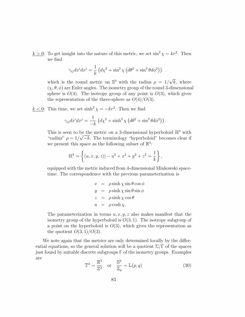
k > 0: To get insight into the nature of this metric, we set sin2 χ = kr2. Thenwe find

γijdxidxj =

1

k

(dχ2 + sin2 χ

(dθ2 + sin2 θdφ2

))which is the round metric on S3 with the radius ρ = 1/

√k, where

(χ, θ, φ) are Euler angles. The isometry group of the round 3-dimensionalsphere is O(4). The isotropy group of any point is O(3), which givesthe representation of the three-sphere as O(4)/O(3).

k < 0: This time, we set sinh2 χ = −kr2. Then we find

γijdxidxj =

1

−k(dχ2 + sinh2 χ

(dθ2 + sin2 θdφ2

)).

This is seen to be the metric on a 3-dimensional hyperboloid H3 with“radius” ρ = 1/

√−k. The terminology “hyperboloid” becomes clear if

we present this space as the following subset of R4:

H3 =

(u, x, y, z)| − u2 + x2 + y2 + z2 =

1

k

,

equipped with the metric induced from 4-dimensional Minkowski space-time. The correspondence with the previous parameterization is

x = ρ sinhχ sin θ cosφ

y = ρ sinhχ sin θ sinφ

z = ρ sinhχ cos θ

u = ρ coshχ.

The parameterization in terms u, x, y, z also makes manifest that theisometry group of the hyperboloid is O(3, 1). The isotropy subgroup ofa point on the hyperboloid is O(3), which gives the representation asthe quotient O(3, 1)/O(3).

We note again that the metrics are only determined locally by the differ-ential equations, so the general solution will be a quotient Σ/Γ of the spacesjust found by suitable discrete subgroups Γ of the isometry groups. Examplesare

T3 =R3

Z3or

S3

Zp= L(p, q) (30)

83

The discrete subgroups are, in those cases, Γ = Z3 ⊂ E(3) (flat case), Γ =Zp ⊂ O(4) (positive curvature). The space L(p, q) is called a Lens-space,and the natural number q which is co-prime to p is related to the precisedefinition of the action of Zp on the 3-sphere: If we identify R4 with C2

and S3 with points (z1, z2) ∈ C2 having |z1|2 + |z2|2 = 1 then any U(2)matrix can be mapped, via this identification, with an orthogonal matrixin O(4) acting on the 3-sphere. If n is a natural number mod p, then itsaction is (z1, z2) 7→ (ein/pz1, e

inq/pz2). The investigation of such quotients isan interesting mathematical problem. Physically, quotients do not seem toplay a role in cosmology so far, so we will not discuss them further.

To summarize, our 4-dimensional spacetime manifold is

M = R×

R3 k = 0, “flat universe”

S3 k > 0, “closed universe”

H3 k < 0, “open universe”

and our 4-dimensional spacetime metric is

ds2 = −dt2 + a(t)2γij(x)dxidxj

= −dt2 + a(t)2

dr2

1− kr2+ r2(dθ2 + sin2 θ dφ2)

.

The spacetime metric depends, up to the parameter7 k ∈ R, only onthe unknown function a(t). This must be determined using Einstein’s equa-tion. For this, we begin by writing down the Ricci tensor components in thecoordinates (xµ) = (t, r, θ, φ). A calculation (excercises) shows:

R00 = −3a

a

R11 =aa+ 2a2 + 2k

1− kr2

R22 = r2(aa+ 2a2 + 2k)

R33 = r2 sin2 θ(aa+ 2a2 + 2k)

To set up Einstein’s equation, we must specify a stress tensor satisfying∇aTab = 0 which is compatible with the spacetime symmetries, i.e. for all

7To be precise, what matters is only the signum of k because we can always normalizek to −1, 0, or +1 by a change of coordinates r 7→ |k|r and a subsequent change of a(t).

84

ψ ∈ G,

ψ?Tab = Tab.

It turns out that the most general such Tab has the fluid form

Tab = ρuaub + P (uaub + gab) ,

where ρ, P are functions only of t and where ua = (dt)a is the tangent fieldto the fluid lines. Equivalently, (uµ) = (1, 0, 0, 0) in our “comoving” (withthe fluid) coordinates (xµ) = (t, r, θ, φ), and

(Tµν) =

ρ 0 0 00 P 0 00 0 P 00 0 0 P

.

We complete our description of matter with an equation of state such as P =wρ, where w ∈ R is constant. One usually requires that |w| ≤ 1 (dominantenergy condition) which includes the case of a “cosmological constant”, Tab =−ρgab with ρ = Lambda > 0 the cosmological constant.

We can now solve Einstein’s equation, which we will use in the tracereversed form Rab = 8πGN (Tab − 1/2gabT ), where T = gabT

ab = −ρ + 3P inour case. However, before investigating this equation directly, it is useful tolook at the consequences of the equation ∇aT

ab = 0 (Bianchi-identity). Thisgives

0 = −ρ− 3a

a(ρ+ P︸ ︷︷ ︸

(1+w)ρ

)

which for ρ > 0 can be solved by

ρ

ρ= −3(1 + w)

a

a

⇔ d

dtlog ρ =

d

dt(log a−3(1+w))

(31)

Henceρ ∝ a−3(1+w) . (32)

85

For some conventional forms of matter this gives

w matter0 pressureless dust ρ ∝ a−3

13

photons ρ ∝ a−4

−1cosmologicalconstant

ρ ∝ a0

We now look at Einstein’s equation directly. The 00-component gives

−3a

a= 4πGN(ρ+ 3P )

whereas any of the ii-components gives

a

a+ 2

(a

a

)2

+2k

a2= 4πGN(ρ− P ).

One can eliminate aa

to get(a

a

)2

=8πGN

3ρ− k

a2(first Friedmann equation)

and

a

a= −4πGN

3(ρ+ 3P ) (second Friedmann equation)

These two equations, first derived by Friedmann and independently by Lemaitre,encode the full dynamics of homogeneous, isotropic spacetimes. We point outthe following very important

Qualitative features:

k < 0: Then, a cannot become zero, which leads to a universe that is foreverexpanding.

k = 0: For any matter having P ≥ 0, ρ must decrease as a increases at leastas rapidly as ρ ≈ a−3 (from the t-component of ∇aT

ab = 0). Thiscauses ρa2 to become zero. Thus, if k = 0, the expansion velocity aapproaches zero as t → ∞. (By contrast, for k < 0, a →

√|k| as

t→∞.)

86

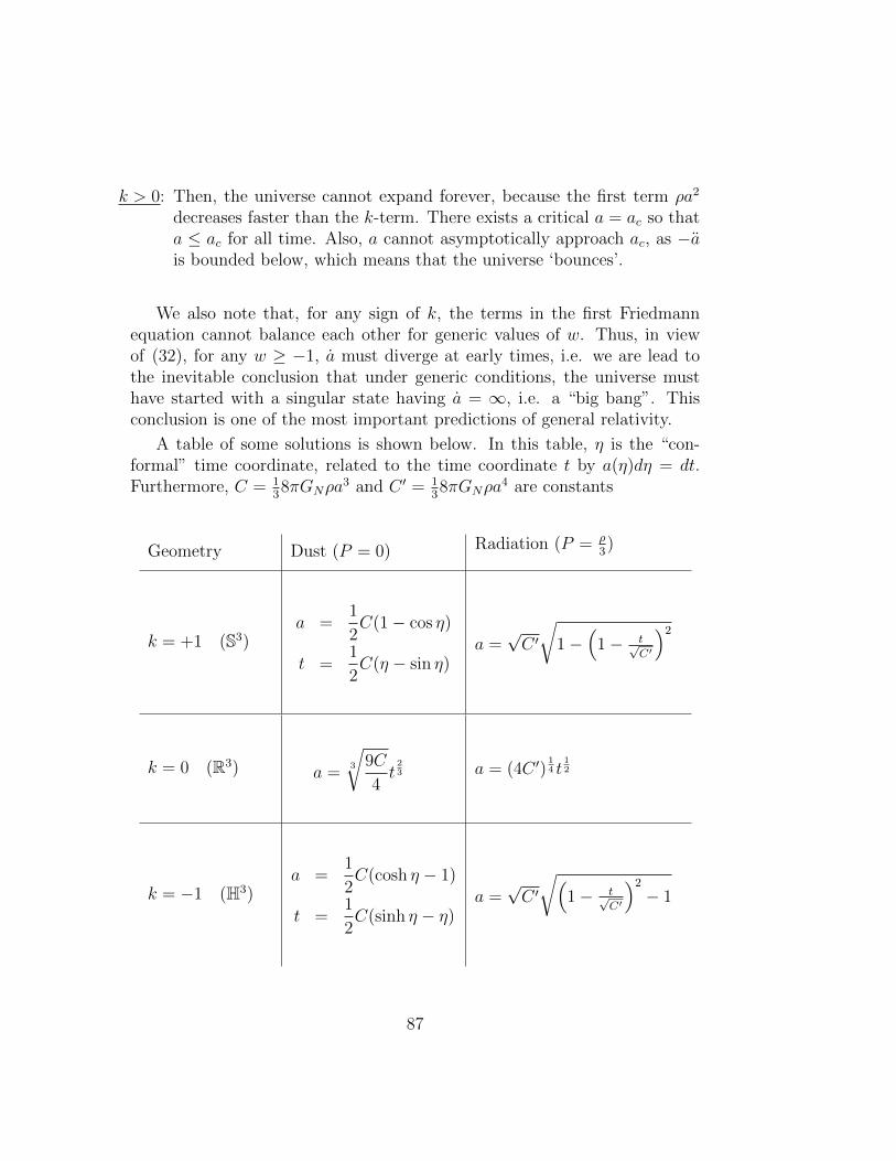
k > 0: Then, the universe cannot expand forever, because the first term ρa2

decreases faster than the k-term. There exists a critical a = ac so thata ≤ ac for all time. Also, a cannot asymptotically approach ac, as −ais bounded below, which means that the universe ‘bounces’.

We also note that, for any sign of k, the terms in the first Friedmannequation cannot balance each other for generic values of w. Thus, in viewof (32), for any w ≥ −1, a must diverge at early times, i.e. we are lead tothe inevitable conclusion that under generic conditions, the universe musthave started with a singular state having a = ∞, i.e. a “big bang”. Thisconclusion is one of the most important predictions of general relativity.

A table of some solutions is shown below. In this table, η is the “con-formal” time coordinate, related to the time coordinate t by a(η)dη = dt.Furthermore, C = 1

38πGNρa

3 and C ′ = 138πGNρa

4 are constants

Geometry Dust (P = 0) Radiation (P = ρ3)

k = +1 (S3)a =

1

2C(1− cos η)

t =1

2C(η − sin η)

a =√C ′√

1−(

1− t√C′

)2

k = 0 (R3) a =3

√9C

4t23 a = (4C ′)

14 t

12

k = −1 (H3)a =

1

2C(cosh η − 1)

t =1

2C(sinh η − η)

a =√C ′√(

1− t√C′

)2

− 1

87

It is also useful to record that, for a flat universe (k = 0) and a generalequation of state P = wρ, with w > −1, we get (exercise)

a(t) ∝ t2

3(1+w) .

The limiting case w = −1 is also interesting and corresponds to a cosmolog-ical constant. In that case, an exponential expansion is found (exercise)

a(t) ∝ etH , (33)

where the constant H = a/a is called “Hubble constant”.One may object that the homogeous and isotropic spacetimes we have

discussed could just be a mathematical exercise without much physical sig-nificance because our symmetry assumptions are clearly not satisfied in re-ality. Indeed, on small scales (e.g. molecular, solar system, or galactic), thestress energy is very far from being distributed in a homogeous and isotropicmanner. Consequently, on such scales also spacetime metric is far from be-ing homogeneous and isotropic (although less so, because the metric is “twoderivatives down” from the stress tensor according to Poisson’s/Einstein’sequation). The hypothesis of homogeneity and isotropy seems, however, avery good approximation on cosmological scales, and the geometries we havedescribed therefore lead to a good description of our universe in the verylarge. Current measurements indicate that k = 0 (or very nearly so) andthat the scale factor appears to have been of the exponential type in theearly cosmos (big bang, inflation), followed by a power law epoch (radiationdominated, then dust), and then followed again by an exponential type epoch.This behavior of the scale factor is incompatible with Einstein’s equations ifonly conventional, baryonic, matter is assumed to be present. In particular,to get an exponential type expansion, we would need matter that is at leastvery similar to a “cosmological constant”, as we have seen. The origin ofsuch a hypothetical kind of matter component is still under discussion. Atany rate, the prediction of a dynamical cosmos (for any type of matter) isone of the, if not the, most remarkable predictions of General Relativity.

12.1 Redshift in cosmological spacetimes

A simple, but very important effect in an expanding universe is the phe-nomenon of redshift. Let us consider a light ray, following an affinely param-eterized null geodesic with ‘wave vector’ ka. The frequency ω measured by

88

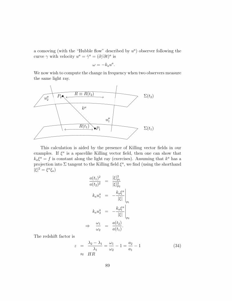
a comoving (with the “Hubble flow” described by ua) observer following thecurve γ with velocity ua = γa = (∂/∂t)a is

ω = −kaua.

We now wish to compute the change in frequency when two observers measurethe same light ray.

kµ

R(t1)

R ≡ R(t2)

P1

P2uµ2

uµ1

Σ(t2)

Σ(t1)

This calculation is aided by the presence of Killing vector fields in ourexamples. If ξa is a spacelike Killing vector field, then one can show thatkaξ

a = f is constant along the light ray (exercises). Assuming that ka has aprojection into Σ tangent to the Killing field ξa, we find (using the shorthand|ξ|2 = ξaξa)

a(t1)2

a(t2)2=|ξ|2p1|ξ|2p2

kaua1 = −kaξ

a

|ξ|

∣∣∣∣∣p1

kaua2 = −kaξ

a

|ξ|

∣∣∣∣∣p2

⇒ ω1

ω2

=a(t2)

a(t1).

The redshift factor is

z =λ2 − λ1

λ1

=ω1

ω2

− 1 =a2

a1

− 1 (34)

≈ HR

89

where R is the distance which is ≈ t2 − t1 for nearby galaxies. For a flatuniverse (k = 0) this is

R = a(t)√x2 + y2 + z2 = geodesic distance.

Another way to state (34) is

a1

a2

=a(emitted)

a(observed)=

1

1 + z.

The ‘physical’= geodesic distance R on a given slice between two pointsis of little empirical interest, since we can only observe objects in our pastlightcone. A more useful notion of distance is the “luminosity distance”, dL,defined as

d2L =

L

4πF. (35)

Here L is the absolute luminosity and F is the flux seen by the observer. ForMinkowski space, dL = R since in that case the area of a sphere of the physicalradius R is 4πR2 = A, that is F

L= 1

Ain a flat space (a(t) ≡ 1, k = 0). On the

other hand, in an expanding (k = 0) Friedmann-Lemaıtre-Robertson-Walkeruniverse, we have instead

F

L=

1

(1 + z)2A

since the photons arriving at t2 are (1 + z)−1 times less energetic (Eph =hν = ~ω) and the rate of emission also goes down by the same factor. Thus,

dL = (1 + z)R.

Because (kµ) = (1, R, 0, 0) is null we must have 1 = a2R2 and hence R = 1a.

Then,

R = R(t2) = a(t)√x2 + y2 + z2

=

ˆ t2

t1

R(t)dt

=

ˆ t2

t1

dt

a(t)

=

ˆ a2

a1

da

a2H(a),

90

or, with dz = −daa2

R =

ˆ z1

z2

dz

H(z)

=

ˆ z

0

dz′

H(z′)

⇒ dL = (1 + z)

ˆ z

0

dz′

H(z′).

It is common to use the first Friedmann equation – or rather its obviousgeneralization to several species of “particles” – in order to replace H2 by

H2 =8πGN

3

∑species i

ρi.

Assuming that each species evolves according to a power law, we find

ρi = ρi,todaya−ni

where ρi,today is the matter density at t2 (today). Assuming without loss ofgenerality that a2 = 1 we find

H(z) =

√8πGN

3

(∑i

ρi,today(1 + z)ni

) 12

⇒ H(z)

Htoday

=

(∑i

Ωi,today(1 + z)ni

) 12

where Ωi(t) ≡ 8πGN3

ρi(t)H(t)2

. Then we get

dL(z) =1 + z

Htoday

ˆ z

0

dz′

(∑

i Ωi,today(1 + z′)ni)12

In practice, we measure dL(z) for large redshifts z and extract Ωi,today andHtoday. For that, we need objects with known intrinsic luminosity L, such astype IIa supernovae.

91

12.2 Particle Horizons

Another important feature of expanding universes is the possible existenceof “particle horizons”. This is most easily demonstrated for flat universes,k = 0, where the metric is

g = −dt2 + a(t)2(dx2 + dy2 + dz2). (36)

Let us introduce again the conformal time parameter η by

η =

ˆ t

t0

dt′

a(t′)

(dη

dt=

1

a(t)⇔ adη = dt

). (37)

from which it follows that

ds2 = a(η)2−dη2 + dx2 + dy2 + dz2︸ ︷︷ ︸

Minkowski-space

(38)

We see that writing the metric in terms of η has the advantage that itsrelationship with Minkowski space becomes manifes: It is “conformal” toMinkowski spacetime, or possible a subset thereof.

Due to the conformal factor a(η)2, geodesics in Minkowski space in generaldo not in general coincide with the geodesics of gab. However, the conformalfactor preserves the causal character of a curve, and therefore the causalrelationships in spacetime. In particular, we may ask whether it is possiblefor two points p, p′ in spacetime to be such that their causal pasts (i.e. theset of all points that can be reached by past directed timelike or null curves)are disjoint. It is clear form the following picture that this will be the caseif and only if the parameter η has a finite range for negative values, whichin turn will be the case if and only if

´ t1t

dt′

a(t′)converges to a finite value for

t→ t0.Whether or not this is the case therefore depends on the behavior of a(t)

near t = t0, which is in turn determined by the equation of state. Indeed,

recall that for P = wρ, we had a(t) ∝ t2

3(w+1) (choosing t0 = 0) so theintegral is finite in particular for all w ≥ 0 (e.g. dust, a ∝ t2/3, or radiation,a ∝ t1/2.) If there are points p, p′ with disjoint causal past, then a particleat p could never have been in contact with a particle at p′ – one says that“there are particle horizons”. Thus, we get regions in spacetime which arecausally disjoint, and for this reason, will not have had the opportunityto equilibrate with each other. Current observations seem to exclude the

92

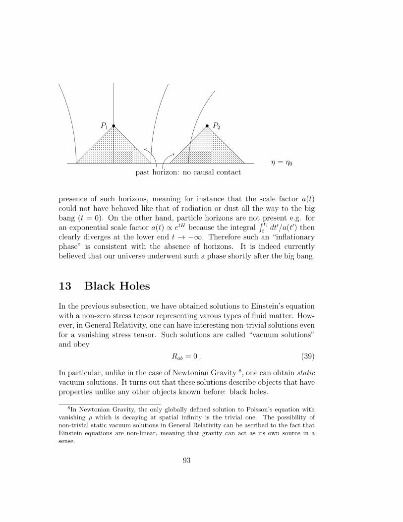
P1 P2

η = η0

past horizon: no causal contact

presence of such horizons, meaning for instance that the scale factor a(t)could not have behaved like that of radiation or dust all the way to the bigbang (t = 0). On the other hand, particle horizons are not present e.g. foran exponential scale factor a(t) ∝ etH because the integral

´ t1tdt′/a(t′) then

clearly diverges at the lower end t → −∞. Therefore such an “inflationaryphase” is consistent with the absence of horizons. It is indeed currentlybelieved that our universe underwent such a phase shortly after the big bang.

13 Black Holes

In the previous subsection, we have obtained solutions to Einstein’s equationwith a non-zero stress tensor representing varous types of fluid matter. How-ever, in General Relativity, one can have interesting non-trivial solutions evenfor a vanishing stress tensor. Such solutions are called “vacuum solutions”and obey

Rab = 0 . (39)

In particular, unlike in the case of Newtonian Gravity 8, one can obtain staticvacuum solutions. It turns out that these solutions describe objects that haveproperties unlike any other objects known before: black holes.

8In Newtonian Gravity, the only globally defined solution to Poisson’s equation withvanishing ρ which is decaying at spatial infinity is the trivial one. The possibility ofnon-trivial static vacuum solutions in General Relativity can be ascribed to the fact thatEinstein equations are non-linear, meaning that gravity can act as its own source in asense.

93

13.1 Derivation of the Schwarzschild Solution

Given the complexity of Einstein’s equations, it is somewhat surprising thatthis family of static solutions, known as the “Schwarzschild solution”, isactually rather easy to derive. To get started one assumes, as seems evidentlyreasonable, that

1. gab has as its isometry group the group of rotations SO(3) and, ofcourse, that

2. gab is static. This means that there are ‘time-shift’ isometries whoseorbits are orthogonal to a spacelike surface Σ.

[The first assumption can actually be shown to be a consequence of thesecond one – this is known as “Israels theorem”.] One can show that timeshifts and rotations commute, and that there exists a local coordinate system(xµ) = (t, r, θ, φ) such that

g = − f(r)︸︷︷︸ dt2 + h(r)︸︷︷︸free functions

dr2 + r2(dθ2 + sin2 θ dφ2

)︸ ︷︷ ︸metric on S2r

with a time shift acting by t→ t+const and rotations acting on the sphericalpolar coordinates φ and θ in the usual way.

It is not hard, although tedious, to compute the Ricci tensor of thismetric in the coordinates (xµ) = (t, r, θ, φ). The off-diagonal componentsvanish identically, whereas the diagonal components give the equations

0 =1

2

1√fh

[f ′√fh

]′+ (rfh)−1f ′ (40)

0 = −1

2

1√fh

[f ′√fh

]′+ (rh2)−1h′ (41)

0 = − f ′

2fh+ (2h2)−1h′ +

1− 1h

r(42)

Equations (40) and (41) give

f ′

f+h′

h= 0 ⇔ f =

k

h(k > 0 a constant,)

94

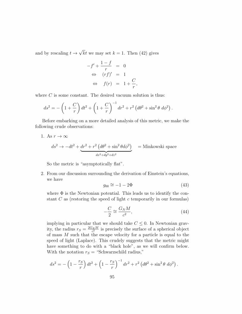
and by rescaling t→√kt we may set k = 1. Then (42) gives

−f ′ + 1− fr

= 0

⇔ (rf)′ = 1

⇔ f(r) = 1 +C

r,

where C is some constant. The desired vacuum solution is thus:

ds2 = −(

1 +C

r

)dt2 +

(1 +

C

r

)−1

dr2 + r2(dθ2 + sin2 θ dφ2

).

Before embarking on a more detailed analysis of this metric, we make thefollowing crude observations:

1. As r →∞

ds2 → −dt2 + dr2 + r2(dθ2 + sin2 θdφ2

)︸ ︷︷ ︸dx2+dy2+dz2

= Minkowski space

So the metric is “asymptotically flat”.

2. From our discussion surrounding the derivation of Einstein’s equations,we have

g00∼= −1− 2Φ (43)

where Φ is the Newtonian potential. This leads us to identify the con-stant C as (restoring the speed of light c temporarily in our formulas)

−C2∼=GNM

c2, (44)

implying in particular that we should take C ≤ 0. In Newtonian grav-ity, the radius rS = 2GNM

c2is precisely the surface of a spherical object

of mass M such that the escape velocity for a particle is equal to thespeed of light (Laplace). This crudely suggests that the metric mighthave something to do with a “black hole”, as we will confirm below.With the notation rS = “Schwarzschild radius,”

ds2 = −(

1− rSr

)dt2 +

(1− rS

r

)−1

dr2 + r2(dθ2 + sin2 θ dφ2

).

95

One gets a better intuition about the size of the constants if one writesfor instance

rS =2GNM

c2≈ 3

(M

M

)km with

M = mass of the sun = 2× 1033g ,

i.e. the sun is vastly bigger than its Schwarzschild radius.

13.2 The redshift effect

Consider two ‘static’ observers, each following a curve of constant r, θ, φ,exchanging a light signal. The tangents are denoted ua1, u

a2, respectively.

P1

P2

uµ1

uµ2

kµ

γ

nullgeodesic

The locally measured frequencies are (compare the corresponding discus-sion in cosmological spacetimes) at two points p1, p2 are:

ω1 = −kaua1∣∣p1

ω2 = −kaua2∣∣p2

We have ua1u1a = −1 = ua2u2a, and the static observers are tangent to theKilling vector field ξa =

(∂∂t

)a. Note that ξaka does not change along the null

geodesic representing the signal, since ξa is Killing, and since ka is geodesic.

96

We may write

ua1 =ξa

|ξ|

∣∣∣p1

ua2 =ξa

|ξ|

∣∣∣p2

where (setting GN = 1 = c in the follwing)

|ξ|2 = −gabξaξb

= 1− 2M

r.

So we find

ω1

ω2

=kau

a1

kaua2=

(kaξa)/|ξ|∣∣p1

(kaξa)/|ξ|∣∣p2

=

√√√√1− 2Mr2

1− 2Mr1

.

If the emitter (1) is closer to the ‘center’ than the receiver (2), r1 < r2, thefrequency will decrease (ω2 < ω1) and hence, by E = ~ω, the energy of aphoton climbing out the gravitational well is decreased. If GNM

c2 r1, r2 then

∆ω

ω≈ −GNM

c2r1

+GNM

c2r2

or ∆E = ~∆ω ≈ ~ωc2

[−GNM

r1

+GNM

r2

].

Since a photon with reduced energy is redder according to Einstein’s formulaE = hν, the effect is called “gravitational redshift”.

13.3 Geodesics

To determine the orbits of material particles and lightrays in the Schwarzschildgeometry, we need to study geodesics. We denote the geodesic by γ : R →M, s 7→ γ(s) and by γa the tangent vector to the geodesic. In coordinates(xµ) = (t, r, θ, φ)

dγµ

ds= γµ = (t, r, θ, φ) .

97

We assume first that the geodesic is timelike, and choose s to be proper time.It follows that there holds

gabγaγb = −1

along the curve. (Proof: act with γc∇c∼= ∂

∂son gabγ

aγb and use γa∇aγb = 0.)

Additionally, the quantities

E = −γa(∂∂t

)aL = γa

(∂∂φ

)a (45)

are also constant along the curve, i.e. independent of s, because (∂/∂t)a and(∂/∂φ)a are Killing fields. (This follows e.g. from eq.??, because the lineelement is independent of t, φ.) Furthermore, since θ 7→ π− θ is an isometryof Schwarzschild, it is consistent to assume that θ(s) = π

2, so θ = 0 along

the geodesic (exercise). Without loss of generality, we may choose γ to bein such an equatorial plane. E has the interpretation of the energy of theparticle, and L that of the angular momentum in the equatorial plane. Fornull geodesics, we have the same constants of motion, but the normalizationcondition is now gabγ

aγb = 0.Substitution of the constants of motion into the normalisation condition

yields, for timelike geodesics,

1

2r2 + V (r) =

1

2E2

where V (r) =1

2− M

r︸︷︷︸Newtonian

term

+L2

2r2︸︷︷︸Angular

momentumbarrier

(centrifugalforce)

−ML2

r3︸ ︷︷ ︸new

.

V (r) can be viewed as the ‘effective potential’ seen by the geodesic. In thenull case, it is given instead by

V (r) =L2

2r2− ML2

r3

The radial motion is thus the same as that of a particle in a potential (V (r)in either case, although the form of the potential is different in the null case.Once the radial motion has been determined, the angular motion is found in

98

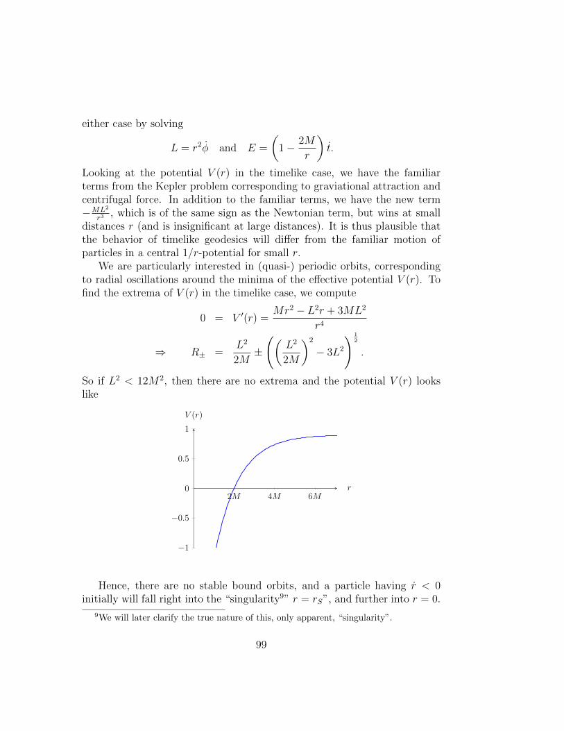
either case by solving

L = r2φ and E =

(1− 2M

r

)t.

Looking at the potential V (r) in the timelike case, we have the familiarterms from the Kepler problem corresponding to graviational attraction andcentrifugal force. In addition to the familiar terms, we have the new term−ML2

r3, which is of the same sign as the Newtonian term, but wins at small

distances r (and is insignificant at large distances). It is thus plausible thatthe behavior of timelike geodesics will differ from the familiar motion ofparticles in a central 1/r-potential for small r.

We are particularly interested in (quasi-) periodic orbits, correspondingto radial oscillations around the minima of the effective potential V (r). Tofind the extrema of V (r) in the timelike case, we compute

0 = V ′(r) =Mr2 − L2r + 3ML2

r4

⇒ R± =L2

2M±

((L2

2M

)2

− 3L2

) 12

.

So if L2 < 12M2, then there are no extrema and the potential V (r) lookslike

2M 4M 6M

−1

−0.5

0

0.5

1

r

V (r)

Hence, there are no stable bound orbits, and a particle having r < 0initially will fall right into the “singularity9” r = rS”, and further into r = 0.

9We will later clarify the true nature of this, only apparent, “singularity”.

99

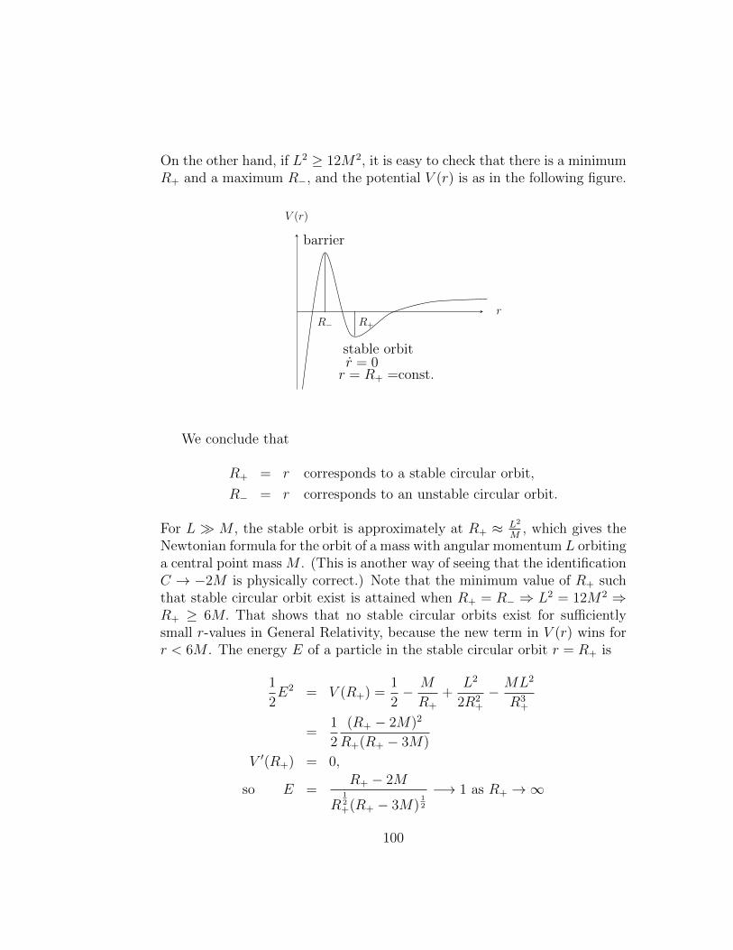
On the other hand, if L2 ≥ 12M2, it is easy to check that there is a minimumR+ and a maximum R−, and the potential V (r) is as in the following figure.

R− R+

r

V (r)

barrier

stable orbitr = 0r = R+ =const.

We conclude that

R+ = r corresponds to a stable circular orbit,

R− = r corresponds to an unstable circular orbit.

For L M , the stable orbit is approximately at R+ ≈ L2

M, which gives the

Newtonian formula for the orbit of a mass with angular momentum L orbitinga central point mass M . (This is another way of seeing that the identificationC → −2M is physically correct.) Note that the minimum value of R+ suchthat stable circular orbit exist is attained when R+ = R− ⇒ L2 = 12M2 ⇒R+ ≥ 6M. That shows that no stable circular orbits exist for sufficientlysmall r-values in General Relativity, because the new term in V (r) wins forr < 6M . The energy E of a particle in the stable circular orbit r = R+ is

1

2E2 = V (R+) =

1

2− M

R+

+L2

2R2+

− ML2

R3+

=1

2

(R+ − 2M)2

R+(R+ − 3M)

V ′(R+) = 0,

so E =R+ − 2M

R12+(R+ − 3M)

12

−→ 1 as R+ →∞

100

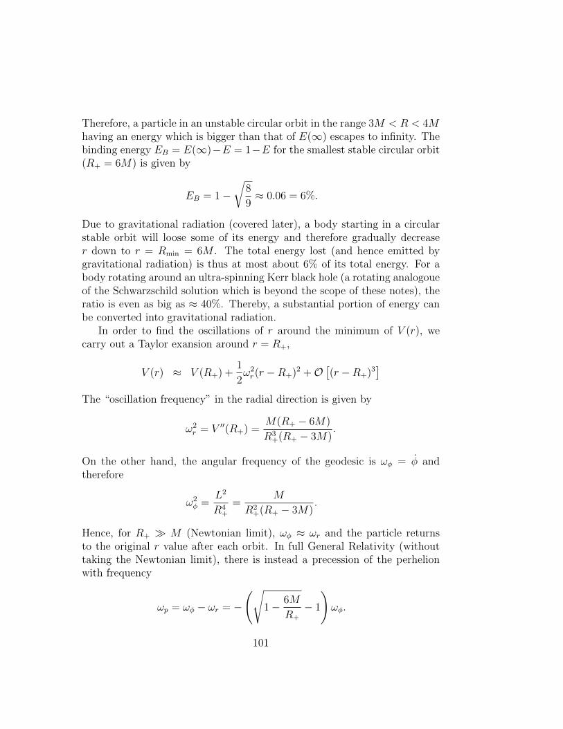
Therefore, a particle in an unstable circular orbit in the range 3M < R < 4Mhaving an energy which is bigger than that of E(∞) escapes to infinity. Thebinding energy EB = E(∞)−E = 1−E for the smallest stable circular orbit(R+ = 6M) is given by

EB = 1−√

8

9≈ 0.06 = 6%.

Due to gravitational radiation (covered later), a body starting in a circularstable orbit will loose some of its energy and therefore gradually decreaser down to r = Rmin = 6M . The total energy lost (and hence emitted bygravitational radiation) is thus at most about 6% of its total energy. For abody rotating around an ultra-spinning Kerr black hole (a rotating analogoueof the Schwarzschild solution which is beyond the scope of these notes), theratio is even as big as ≈ 40%. Thereby, a substantial portion of energy canbe converted into gravitational radiation.

In order to find the oscillations of r around the minimum of V (r), wecarry out a Taylor exansion around r = R+,

V (r) ≈ V (R+) +1

2ω2r(r −R+)2 +O

[(r −R+)3

]The “oscillation frequency” in the radial direction is given by

ω2r = V ′′(R+) =

M(R+ − 6M)

R3+(R+ − 3M)

.

On the other hand, the angular frequency of the geodesic is ωφ = φ andtherefore

ω2φ =

L2

R4+

=M

R2+(R+ − 3M)

.

Hence, for R+ M (Newtonian limit), ωφ ≈ ωr and the particle returnsto the original r value after each orbit. In full General Relativity (withouttaking the Newtonian limit), there is instead a precession of the perhelionwith frequency

ωp = ωφ − ωr = −

(√1− 6M

R+

− 1

)ωφ.

101

For R+ M we get to the lowest non-vanishing order

ωp ≈3MωφR+

≈ 3M

R+

(M

R3+

) 12

=3M

32

R52+

,

and restoring c,GN :

ωp ≈3(GNM)

32

c2R52+

.

For Mercury, this gives (taking also the eccentricity of the orbit into ac-count) ωp(') = 43′′

100a. It is surprising – and a lucky coincidence – that this

minute precession had been observed around the time General Relativity wasconceived. Newtonian calculations, including even the perturbations by theother planets, which could be carried out thanks to the enormous advancesin Celestial Mechanics in the end of the 19th century, could not accountfor this effect, whereas General Relativity could. Hence, the prediction ofthe perihelion precession of Mercury was historically the first test of GeneralRelativity.

A similar analysis can be carried out for null-geodesics “skimming thesurface at the Schwarzschild radius”, and leads to the prediction of lightbending – another early test of General Relativity (exercises).

13.4 Kruskal extension

In order to gain insight into the nature of the apparent singularity of theSchwarzschild metric at r = rS, we next consider radially outgoing null-geodesics, which exist due to the symmetries of the line element. As before,our geodesics are denoted by (γµ(s)) = (t(s), r(s), θ(s), φ(s)), and for radialgeodesics (γµ) = (t, r, 0, 0). The null-condition leads to

0 = gabγaγb

= −(

1− 2M

r

)t2 +

r2

1− 2Mr

ordt

dr= ±

(r

r − 2M

)102

or

t = ±r∗ + const.

with r∗ = r + 2M log( r

2M− 1)⇒ dr∗ =

dr

1− 2Mr

.

It seems a good idea to try to rewrite the line element in terms of coordinatesobtained from the affine parameters along radial null geodesics. Since we havejust seen that the latter are defined by the conditions ±r∗+ t = constant andφ, θ = constant, the appropriate coordinates are u = t − r∗, v = t + r∗ (andθ, φ), in terms of which the line element becomes

ds2 = −(

1− 2M

r

)dudv + r2(dθ2 + sin2 θ dφ2) .

Here r is now viewed as a function of u and v; explicitly

r + 2M log( r

2M− 1)

= r∗ =v − u

2.

We now make further transformations

U = − exp

(−u4M

)≡ T −X ,

V = exp( v

4M

)≡ T +X .

The relationship between the original coordinates (t, r) and the new ones(T,X) is summarized in the following equations( r

2M− 1)

exp( r

2M

)= X2 − T 2 , (46)

t

2M= log

(T +X

X − T

)= 2 arctanh

T

X. (47)

Changing to the coordinates (T,X) leads to the “Kruskal form” of the lineelement

ds2 =32M3

rexp

(− r

2M

)(−dT 2 + dX2) + r2(dθ2 + sin2 θdφ2). (48)

The Kruskal form of the line element shows that r = rS is not a singularity,because we can clearly extend the metric analytically across this value, atleast until r = 0. Thus, the true geometry is the analytically extended man-ifold labelled by the coordinates X,T , and the coordinates on S2, consistentwith r > 0. We see:

103

1. The allowed range of T and X consistent with r > 0 is X2 − T 2 > −1.The value X2 − T 2 = −1 corresponds to r = 0. This is seen to bea true singularity, e.g. by evaluating the “Kretschmann invariant”:RabcdR

abcd →∞.

2. By contrast, r = 2M (r = rS) corresponds to T = ±X, which is not asingularity.

3. The surfaces of constant t corresponds to TX

= constant.

4. At T = 0 = X we have, from equation (46), that

dr∣∣∣T=X=0

=4M

e(XdX − TdT )

∣∣∣X=T=0

= 0

and that gab(dr)b and(∂∂t

)a(when expressed in X,T -coordinates) be-

come co-linear at T = ±X. It follows that ∂(r,t)∂(X,T )

becomes singular

there, too, showing that (r, t) are ‘bad coordinates’. The apparent sin-gularity at r = rS in the original coordinates is hence due to a badchoice of coordinates.

The causal structure of Schwarzschild following from equation (48) is bestillustrated in a diagram in which the (φ, θ)-coordinates are suppressed.

104

T

X

r = 0

r = 0

T = X

T = −X

t =constant

Σ

(singularity)

r = 2M

orbits of ∂∂t

I

II

III

IV

1. Region I (excluding r = 2M -lines) corresponds to the original coordi-nate range r > 2M (‘exterior ’).

2. Region II has the property that no lightlike-future-directed curves canenter the exterior region I (‘black hole’).

3. Region III has the property that no lightlike-future-directed curves canstay within that region forever (‘white hole’).

4. Region IV has properties identical to those of region I. If we considerthe metric h = hijdx

idxj with (xi) = (X, θ, φ) induced on Σ = T = 0,we obtain a Riemannian 3-manifold streching between regions I and IV.Its geometry is illustrated in the following figure (for a 2 + 1 version ofSchwarzschild for the sake of visualization). The embedding into flatspace is intended to be such that the induced metric corresponds to

105

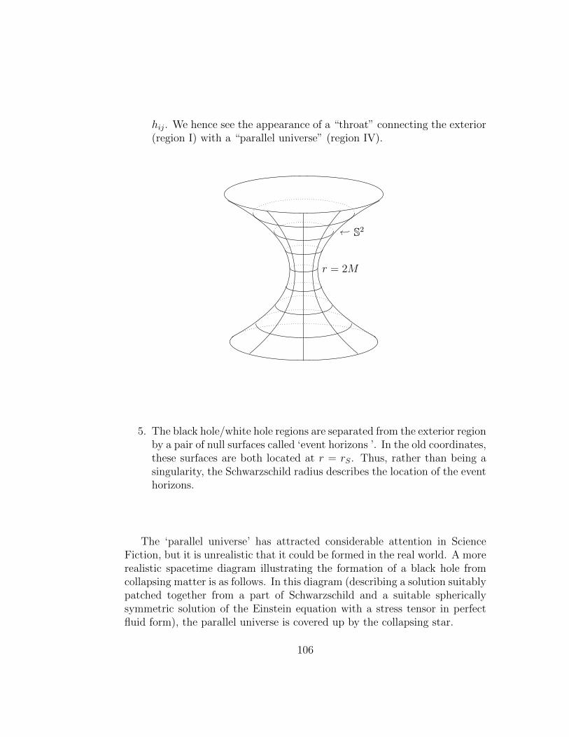
hij. We hence see the appearance of a “throat” connecting the exterior(region I) with a “parallel universe” (region IV).

r = 2M

S2

5. The black hole/white hole regions are separated from the exterior regionby a pair of null surfaces called ‘event horizons ’. In the old coordinates,these surfaces are both located at r = rS. Thus, rather than being asingularity, the Schwarzschild radius describes the location of the eventhorizons.

The ‘parallel universe’ has attracted considerable attention in ScienceFiction, but it is unrealistic that it could be formed in the real world. A morerealistic spacetime diagram illustrating the formation of a black hole fromcollapsing matter is as follows. In this diagram (describing a solution suitablypatched together from a part of Schwarzschild and a suitable sphericallysymmetric solution of the Einstein equation with a stress tensor in perfectfluid form), the parallel universe is covered up by the collapsing star.

106

I

II

collapsing matter(FLRW-metric

out to some r(t))

origin of

coordinates

r = 2Msingularity

14 Linearized Gravity and Gravitational Ra-

diation

In the preceeding sections we have described (i) a dynamical solution to Ein-stein’s equations with no “spatial excitations” (cosmological solutions) and(ii) a static solution with non-trivial spatial dependence (Schwarzschild blackhole). A generic solution has spatial excitations that evolve in time. It turnsout that the evolution equations implied by Einstein’s equations have thecharacter of a “quasi-linear” wave equation. The analysis of such equationsis beyond the scope of these notes, see for example [?] for a detailed exposi-tion. However, it turns out that one can derive, without major difficulties,the solutions describing small “linear” perturbations of Minkowski spacetime.These solutions describe gravitational waves. They have no counterpart inNewtonian Gravity and are, in this sense, a genuinely new prediction of Gen-eral Relativity. This prediction is currently being tested with gravitationalwave interferometers such as LIGO, GEO600 and VIRGO. It is conceivablethat a detection might occur within this decade.

107

14.1 Gravitational waves in empty space

We first describe how to obtain the linearized Einstein equations. Mathemat-ically, the best way to proceed is to suppose that one has a (differentiable)1-parameter family gab(s)s∈R of solutions to the Einstein equations, e.g. invacuum,

Rab(s) = 0

where we mean the Ricci tensor of the metric gab(s). We think of gab ≡ gab(0)as the “background”, and we think of gab(s), |s| 1 as small “deviations”or “perturbations” of this background. The first order deviation is just thederivative with respect to s at s = 0,

γab ≡∂

∂sgab(s)

∣∣∣∣s=0

.

γab is referred to as the “linear perturbation”. In General Relativity, theobservable is not the metric, but its “gauge equivalence class”, i.e. the setof all metrics related to gab by a diffeomorphism, ψ∗gab. Consequently, ifψ(s)s∈R is a (differentiable) 1-parameter family of diffeomorphisms of M ,then gab(s)s∈R and ψ(s)∗gab(s)s∈R should be viewed as physically describ-ing the same families of spacetimes. Thus, at the linearized level (i.e. differ-entiating with respect to s and making use of the notion of Lie-derivatives),we find that γab and γab + LXgab physically describe the same perturbation,where Xa is the generator of the family of diffeomorphisms at s = 0. Onealso says that the “gauge-invariance” at the linearized level is

γab → γab + LXgab = γab +∇aXb +∇bXa .

The linearized (vacuum) Einstein equations are obtained by simply differen-tiating the Einstein equations with respect to s at s = 0, namely

Rab ≡∂

∂sRab(s)

∣∣∣∣s=0

= 0 .

The left side of this equation is readily calculated in terms of gab and γab,but we will not give the general expression here. Rather we will specializedirectly to the case of interest for us in which gab = ηab is Minkowski space.With gab(s) = ηab + sγab +O(s2), we get:

gab = −γab (49)

Γcab =1

2ηcd (∂aγbd + ∂bγad − ∂dγab) , (50)

108

where here and in the following, we adopt the convention that indices onexpressions related to γab are raised and lowered with ηcd, and where anoverdot means a derivative with respect to s at s = 0. With these expressionsat hand, we find that the linearized Riemann tensor is

Reabc = −1

2ηcd∂e (∂aγbd + ∂bγad − ∂dγab)− (a↔ e) ,

and we find that the linearized Ricci tensor is

Rab = ∂c∂(bγa)c −1

2∂c∂cγab −

1

2∂a∂bγ ,

where γ = ηabγab and where parenthesis denote symmetrization of the re-spective tensor indices. We then get for the linearized Einstein tensor:

Gab = Rab −1

2ηabRcdη

cd

= ∂c∂(bγa)c −1

2∂c∂cγab −

1

2∂a∂bγ −

1

2ηab(∂c∂dγcd − ∂c∂cγ

). (51)

Using the formulae for Lie derivatives, the linearized gauge transformationon a Minkowski background is

γab → γab + ∂aXb + ∂bXa ,

where Xa is an arbitrary (smooth) tensor. To investigate how these quantitieschange under a linearized gauge transformation We note that, for instance,Rabcd[ψ

∗g] = ψ∗Rabcd[g] for any metric gef and any diffeomorphism M (thisof course expresses the “general covariance” of quantities like the Riemanntensor.) Using the formulas for the Lie-derivate, we consequently have for alinear perturbation of any background the transformation formula

Rabcd → Rabcd + LXRabcd ,

Gab → Gab + LXGab , (52)

and similarly for any other tensor field that is locally and constructed out ofgab,∇a, g

ab. We can conclude from such formulae that any linearized quan-tity whose counterpart vanishes in the background, is automatically gaugeinvariant. In particular, if Gab = 0 in the background, then the linearizedEinstein tensor Gab is gauge invariant. In Minkowski spacetime Rabcd = 0,

109

so even the linearized Riemann tensor Rabcd is gauge invariant. We will nowderive a wave equation for this quantity. For this, we look at the linearizedBianchi identities on Minkowski spacetime. They read

∂[aRbc]de = 0 (53)

∂dRabcd = 0 . (54)

We now apply ∂a to the first equation and use the second equation as wellas Rab = 0. Then we get, indeed,

∂a∂aRbcde = 0 .

To analyze the effect of metric perturbations on the motion of test-observers,we choose the wave vector ωka, where

ka =1√2

[(∂

∂t

)a−(∂

∂z

)a]and consider a corresponding plane fronted wave-like perturbation γab movingin the z-direction with spacetime dependence sin[ω(t+z)]. The correspondinglinearized Riemann tensor is then a solution to the wave equation. To derivethe motion of test-observers on this background, it is convenient to introduceanother null vector la

la =1√2

[(∂

∂t

)a+

(∂

∂z

)a],

and define the symmetric tensor

Ωab ≡1

2Racbdl

cld ⇒ ∂c∂cΩab = 0 .

The quantity Ωab has the following properties:

1. Ωab is invariant under linear gauge transformations.

2. Ωabkb = 0 (from the second linearized Bianchi identity and the depen-

dence Rabcd ∝ sin[ω(kexe)]), and Ωablb = 0 (from R(ab)cd = Rab(cd) = 0).

3. Ωabηab = 0 (from Rab = 0), and Ωab = Ωba (from Rabcd = Rcdab).

110

It follows that Ωab is a trace-free, symmetric tensor having components onlyin the x, y-directions. We can therefore write

Ωab = ω2h+ · ε+ab + h× · ε×ab

sin[ω(t+ z)] ,

where ε+ab, ε×ab forms a basis of such tensors; in coordinates

ε+ab = (dx)a(dx)b − (dy)a(dy)b , ε×ab = (dx)a(dy)b + (dx)b(dy)a ,

and where h+, h× ∈ R are the amplitues of the “polarizations” +,×. Ininertial coordinates the polarization tensors for a wave moving in the z-direction are

(ε+µν) =

0 0 0 00 1 0 00 0 −1 00 0 0 0

(ε×µν) =

0 0 0 00 0 1 00 1 0 00 0 0 0

.

We now consider the effect of a plane gravitational wave moving in thez-direction on the motion of test-observers. The motion of the test-observersis described by the geodesic deviation equation. We need to understand whatthis equation tells us at the order of approximation considered here. For this,it is best again to think about a family of metrics gab(s) = ηab+sγab+O(s2).We consider geodesics starting on a slice Σ = t = 0 which are initiallyparallel with tangent vector T a = (∂/∂t)a. The evolution of these geodesicstakes place in the s-dependent spacetime gab(s). For s = 0, the metric is flatspace and the geodesic deviation vector vanishes identically. Consequently,the geodesic deviation vector is Taylor expanded to second order in s as

Xa(s, t) = sXa(t) +1

2s2Xa(t) +O(s3),

where an overdot again stands for a derivative with respect to the parameter s(and not the time parameter, t). We next differentiate the geodesic deviationequation several times with respect to s at s = 0. In principle, all quantitiesin the geodesic deviation equation depend upon the parameter s, includingalso T a = T a(s, t), the tangent to the geodesics, because the metric gab(s)depends upon s. Taking one s-derivative of the geodesic deviation equationgives

∂2

∂t2Xa(t) = 0 ,

111

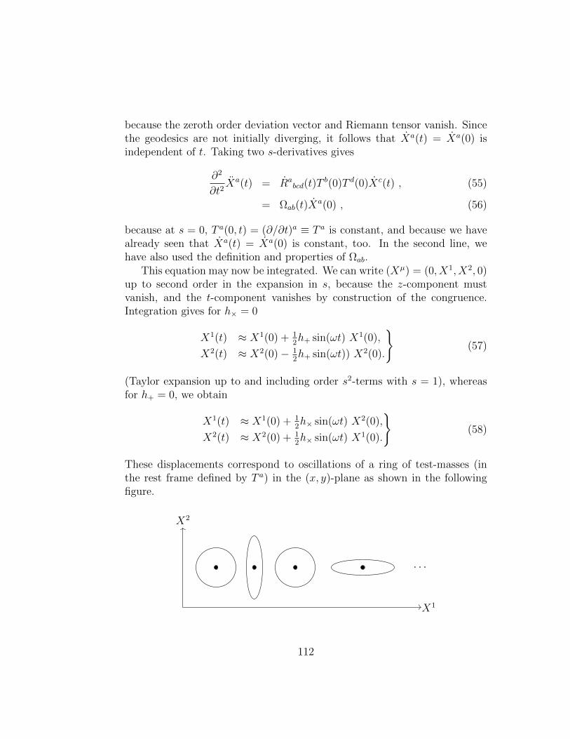
because the zeroth order deviation vector and Riemann tensor vanish. Sincethe geodesics are not initially diverging, it follows that Xa(t) = Xa(0) isindependent of t. Taking two s-derivatives gives

∂2

∂t2Xa(t) = Ra

bcd(t)Tb(0)T d(0)Xc(t) , (55)

= Ωab(t)Xa(0) , (56)

because at s = 0, T a(0, t) = (∂/∂t)a ≡ T a is constant, and because we havealready seen that Xa(t) = Xa(0) is constant, too. In the second line, wehave also used the definition and properties of Ωab.

This equation may now be integrated. We can write (Xµ) = (0, X1, X2, 0)up to second order in the expansion in s, because the z-component mustvanish, and the t-component vanishes by construction of the congruence.Integration gives for h× = 0

X1(t) ≈ X1(0) + 12h+ sin(ωt) X1(0),

X2(t) ≈ X2(0)− 12h+ sin(ωt)) X2(0).

(57)

(Taylor expansion up to and including order s2-terms with s = 1), whereasfor h+ = 0, we obtain

X1(t) ≈ X1(0) + 12h× sin(ωt) X2(0),

X2(t) ≈ X2(0) + 12h× sin(ωt) X1(0).

(58)

These displacements correspond to oscillations of a ring of test-masses (inthe rest frame defined by T a) in the (x, y)-plane as shown in the followingfigure.

X1

X2

· · ·

112

We summarize our discussion as follows. At the linearized level, pertur-bations of Minkowski space (or rather, their corresponding Riemann tensor)obey a homogeneous wave equation. A plane wave moving in the z-directiongives rise to an oscillation of a ring of test-masses in the (x, y)-plane. Theoscillation pattern depends on the polarization, +, respectively ×, and canpotentially be observed e.g. by interferometers, as LIGO, VIRGO, GEO600are indeed attempting to do. Since the physcial degrees of freedom of thegravitational field (i.e. gauge invariant information) can only manifest then-selves via their influence on test-masses, we can say that a gravitational wavehas “two degrees of freedom” (per wave vector), namely +,×.

14.2 Sources of gravitational waves

We next discuss the production of gravitational waves. For this, we needto study the linearized Einstein equations with a non-trival stress tensor Tabrepresenting the source. It is convenient at this stage to introduce the “tracereversed” variable

γab = γab −1

2ηabγ ⇔ γab = γab −

1

2γηab .

In terms of this variable, the linearized Einstein tensor takes the form

Gab = −1

2∂c∂cγab + ∂c∂(aγb)c −

1

2ηab∂

c∂dγcd

= 8πGN Tab .

We have put a stress energy tensor on the right side. To be consistent atthe linearized level, this should satisfy ∂aTab = 0. Recall that the gaugeinvariance of General Relativity at the linearized level is

γab → γab + ∂aXb + ∂bXa .

where the expression for the Lie derivative of the Minkowski metric has beenused, and recall that Gab is gauge invariant. We may use the gauge invarianceto fix a particularly useful representer in the gauge equivalence class of γab.For this, we note that under a gauge transformation

∂cγac → ∂cγac + ∂c∂cXa .

Because ∂c∂c is the wave operator in Minkowski spacetime, we can find asolution Xa to the equation ∂c∂cXa = −∂cγca. Using any Xa satisfying this

113

equation in the gauge transformation, it follows that the gauge-transformedlinear perturbation has ∂cγac = 0. This gauge is called the “Lorentz gauge”,by analogy with Maxwell’s equations. In the Lorentz gauge, the linearizedEinstein equation simply becomes

γab = −16πGN Tab

We see again that the evolution equation for linear perturbations is a waveequation. It can be shown that the residual gauge freedom can be used upto impose even more stringent gauge conditions such as γ = 0 = γabT

b (inthe source free region where Tab = 0), see [Wald 1984] for a discussion. Fora plane gravitational wave in empty space with wave-vector ωka as in thepreceeding section, we thus get the conditions γ = γabT

b = γabkb = 0. This

reduces the number of independent components of γab from 10 down to 2(there are 8 independent gauge conditions). Thus, we see again that thegravitational field has 2 degrees of freedom per ωka, corresponding to +,×polarized waves. We next discuss the

Production of gravitational waves: Significant amounts of gravitationalwaves are produced in Nature by binary systems with large masses and largeorbital frequencies, for instance by binaries of neutron stars or black holes(especially during their merger phase), but also in the Early Universe. Herewe imagine a localized source such as a binary. The (in principle very com-plicated) structure of the source is supposed to be encoded in the matterstress tensor, Tab. We imagine that Tab has compact support in a space-time region where for instance a collapse or merger takes place. Fromγab = −16πGN Tab we obtain

γab = −16πGN ∆ret ∗ Tab .

Here, the star is convolution, and ∆ret is the retarded propagator

∆ret(t,x) = − 1

2πΘ(−t)δ(t2 − ‖x‖2)

114

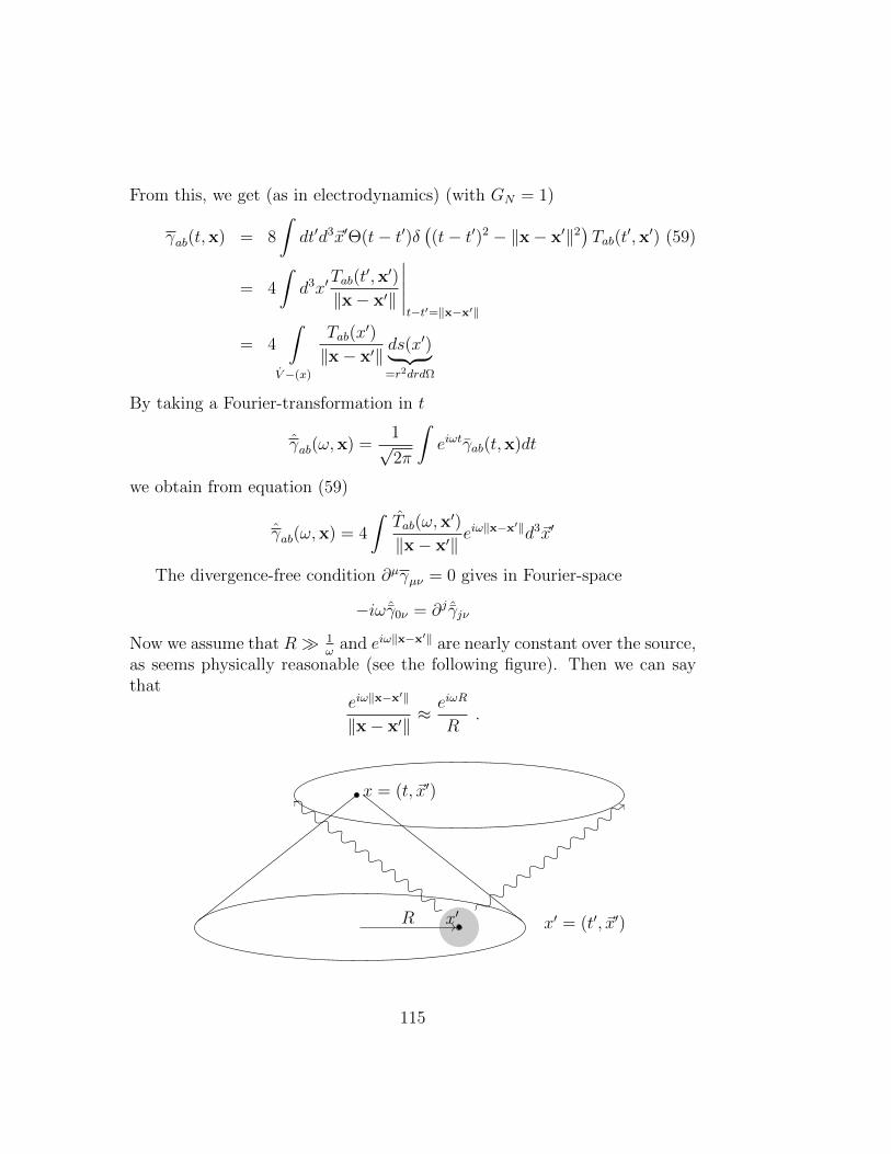
From this, we get (as in electrodynamics) (with GN = 1)

γab(t,x) = 8

ˆdt′d3~x′Θ(t− t′)δ

((t− t′)2 − ‖x− x′‖2

)Tab(t

′,x′) (59)

= 4

ˆd3x′

Tab(t′,x′)

‖x− x′‖

∣∣∣∣∣t−t′=‖x−x′‖

= 4

ˆ

V−(x)

Tab(x′)

‖x− x′‖ds(x′)︸ ︷︷ ︸=r2drdΩ

By taking a Fourier-transformation in t

γab(ω,x) =1√2π

ˆeiωtγab(t,x)dt

we obtain from equation (59)

γab(ω,x) = 4

ˆTab(ω,x

′)

‖x− x′‖eiω‖x−x

′‖d3~x′

The divergence-free condition ∂µγµν = 0 gives in Fourier-space

−iωˆγ0ν = ∂j ˆγjν

Now we assume that R 1ω

and eiω‖x−x′‖ are nearly constant over the source,

as seems physically reasonable (see the following figure). Then we can saythat

eiω‖x−x′‖

‖x− x′‖≈ eiωR

R.

x = (t, ~x′)

x′ x′ = (t′, ~x′)R

115

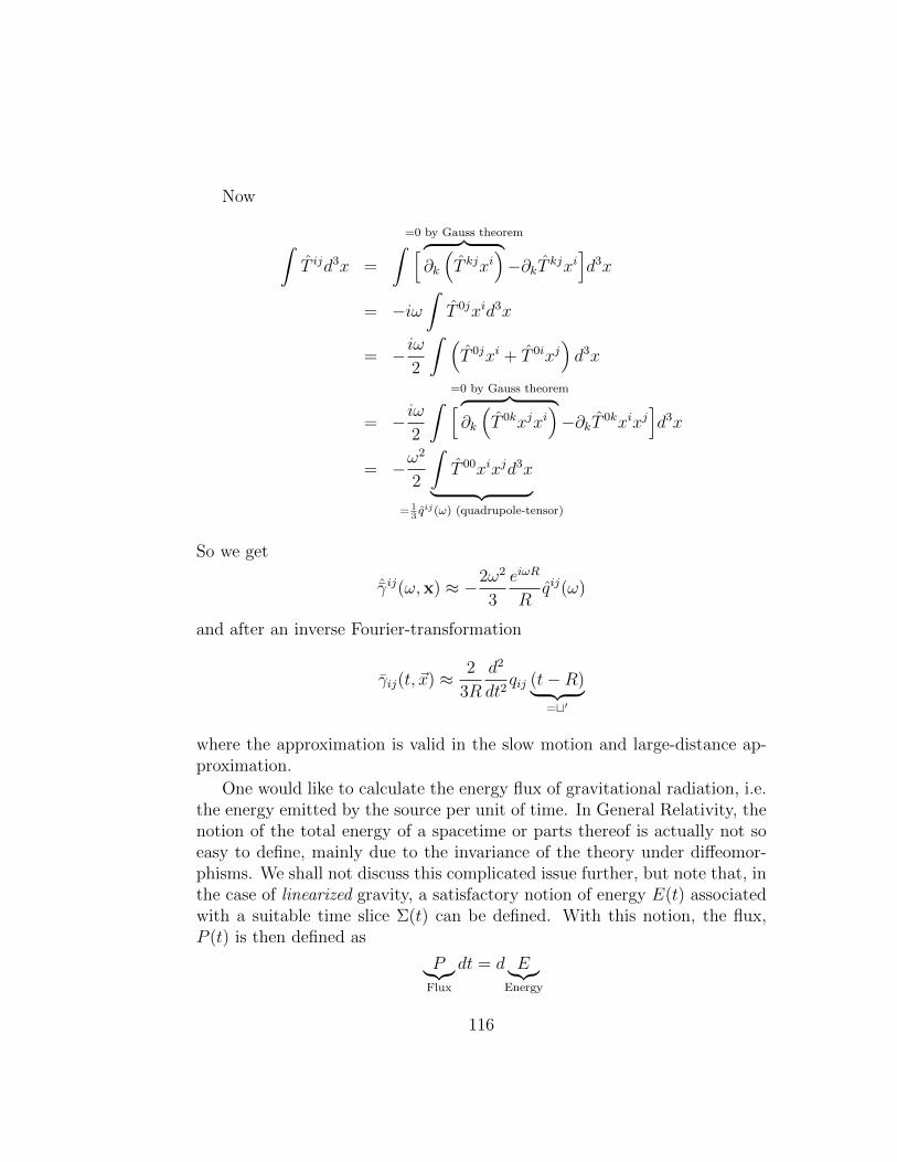
Now

ˆT ijd3x =

ˆ [=0 by Gauss theorem︷ ︸︸ ︷∂k

(T kjxi

)−∂kT kjxi

]d3x

= −iωˆT 0jxid3x

= −iω2

ˆ (T 0jxi + T 0ixj

)d3x

= −iω2

ˆ [=0 by Gauss theorem︷ ︸︸ ︷∂k

(T 0kxjxi

)−∂kT 0kxixj

]d3x

= −ω2

2

ˆT 00xixjd3x︸ ︷︷ ︸

= 13qij(ω) (quadrupole-tensor)

So we get

ˆγij(ω,x) ≈ −2ω2

3

eiωR

Rqij(ω)

and after an inverse Fourier-transformation

γij(t, ~x) ≈ 2

3R

d2

dt2qij (t−R)︸ ︷︷ ︸

=t′

where the approximation is valid in the slow motion and large-distance ap-proximation.

One would like to calculate the energy flux of gravitational radiation, i.e.the energy emitted by the source per unit of time. In General Relativity, thenotion of the total energy of a spacetime or parts thereof is actually not soeasy to define, mainly due to the invariance of the theory under diffeomor-phisms. We shall not discuss this complicated issue further, but note that, inthe case of linearized gravity, a satisfactory notion of energy E(t) associatedwith a suitable time slice Σ(t) can be defined. With this notion, the flux,P (t) is then defined as

P︸︷︷︸Flux

dt = d E︸︷︷︸Energy

116

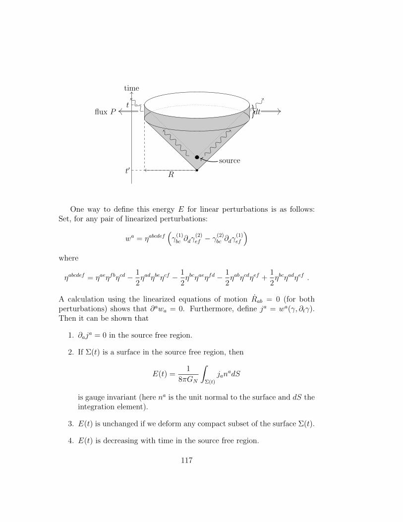
time

t′

t

R

dt

source

flux P

One way to define this energy E for linear perturbations is as follows:Set, for any pair of linearized perturbations:

wa = ηabcdef(γ

(1)bc ∂dγ

(2)ef − γ

(2)bc ∂dγ

(1)ef

)where

ηabcdef = ηaeηfbηcd − 1

2ηadηbeηcf − 1

2ηbcηaeηfd − 1

2ηabηcdηef +

1

2ηbcηadηef .

A calculation using the linearized equations of motion Rab = 0 (for bothperturbations) shows that ∂awa = 0. Furthermore, define ja = wa(γ, ∂tγ).Then it can be shown that

1. ∂aja = 0 in the source free region.

2. If Σ(t) is a surface in the source free region, then

E(t) =1

8πGN

ˆΣ(t)

janadS

is gauge invariant (here na is the unit normal to the surface and dS theintegration element).

3. E(t) is unchanged if we deform any compact subset of the surface Σ(t).

4. E(t) is decreasing with time in the source free region.

117

The proofs of these claims follow from the arguments in [7]. These propertiessuggest that E(t) should be viewed as the energy of the linear perturbationγab at “time t” (in the source free region) if we define Σ(t) as a suitably“asymptotically hyperboloidal” slice approaching a lightcone at “retardedtime”, t. A possible choice is

Σ(t) = (xµ) | (x0 − t)2 −∑j

(xj)2 = 1 .

The corresponding flux P (t) emitted by a gravitational wave in the far regionmay then be calculated. After a very lengthy calculation, it is found that

P (t) =d

dtE(t) ≈ GN

45

3∑i,j=1

(...Qij(t−R)

)2

where Qij = qij − 13δijq is the traceless part of the quadrupole tensor. This

relation is known as the “quadrupole formula” and is to be compared withthe corresponding formula in electromagnetism, involving only the dipolemoment. This difference can be traced back to the difference in the tensorcharacter of both fields.

To get an impression of the order of magnitude of gravitational radiation,we consider an

Example: We consider a binary consisting of point objects A and Bwith equal mass M , distance L in a circular orbit with orbital frequency Ωin the z = 0 plane. The stress tensor of the system is modeled by:

T 00(t, x, y, z) = M δ(z)δ (x− L cos Ωt) δ (y − L sin Ωt)︸ ︷︷ ︸

A

+ δ (x+ L cos Ωt) δ (y + L sin Ωt)︸ ︷︷ ︸B

with all other components equal to 0. (Note that this form is actually incon-sistent with ∂aTab = 0, which is not surprising since it is not really possibleto describe a bound system at the level of linear perturbation theory.) Pro-ceeding despite this obvious inconsistency, we get for the reduced quadrupole

118

(with qij = 3´T 00xixjd

3x)

Qij = qij −1

3δijq

(Qij) =ML2

3

1 + 3 cos 2Ωt 3 sin 2Ωt 03 sin 2Ωt 1− 3 cos 2Ωt 0

0 0 −2

Reinstating c, we get for the flux P of the binary:

Pbinary=− 128

45c5GNM

2L4Ω6 .

The factor Ω6 stems from 6 time derivatives and effectively turns P into anastronomically small number. For masses/lengths of the order of the Earth-Sun system, one finds a flux of about 100 Watts per second. To get anappreciable flux, one needs sources that are very massive and spinning veryfast, and one needs sufficiently long observation times. Such sources are pro-vided for example by pulsars, consisting of a pair of orbiting neutron stars.The orbital frequency Ω is observable to a high precision due to the “light-house effect”. The gravitational radiation produced is sufficient to producean energy loss affecting the orbital frequency. Such a change in the orbitalfrequency has now been observed in several pulsars. The quantitative resultsseem to confirm the quadrupole formula, and hence are a stringent test ofGeneral Relativity.

15 The Global Positioning System

The motivation behind the Global Positioning System is to accurately de-termine positions and times for any events near Earth. To do this, we needto take certain relativistic effects into account. The implementation of theGPS seems to be the first application of General Relativity on a large scalewhich is relevant to a general public because of commercial applications likecar navigation equipment.

The results and presentation in section are mostly based on [1].

15.1 Introduction

Let us ignore gravity for the moment and suppose that we can describe allevents near Earth using inertial coordinates (ct,x) in the sense of Special

119

Relativity. Suppose that we (or an observer O) are at some unknown event(ctO,xO), but we receive radio signals from four sources and informationabout the four events (ctj,xj), j = 1, 2, 3, 4, where these signals originated.In general we can then determine the coordinates (ctO,xO) using a simpletriangulation: because the radio signals travel at the speed of light, the fourequations

tO − tj = c−1‖xO − xj‖, j = 1, 2, 3, 4 (60)

must be satisfied. These four equations allow us to determine the four un-known coordinates, in general.

A few remarks are in order:

1. If the signals are not received at exactly the same time, but at timestO + δj and at positions xO + dj, we can use the equations

tO + δj − tj = c−1‖xO + dj − xj‖, j = 1, 2, 3, 4.

Note that the values for δj can be measured by the local observer (set-ting e.g. δ1 = 0 to eliminate a free constant). In addition we can makereasonable estimates for the vectors dj, because in most applicationsthese are mostly due to the rotation of Earth. (The rotation speed de-pends on the latitude, but it is typically much larger than the speed ofthe observer with respect to Earth.) In this way we reduce the problemagain to four unknowns, which may be obtained from four equations.

2. In the GPS, the sources are artificial satellites in orbit around Earth.There are 24 GPS satellites put into orbit in such a way that at leastfour of them are visible at almost every place and time on Earth. Ifthe orbits of the satellites are known rather accurately as a function oftime, it only remains for the satellite to determine the time, using anon-board clock.

3. In order to determine positions with an accuracy of 1m, we see fromequation (60) that we need to determine times with an accuracy of1mcm

s∼ 3.33 · 10−9s= 3.33ns.

High precision time measurement is one of the main challenges of the GPSsystem, and it is affected by the gravitational field of Earth and the motion ofthe satellites (and the observer O who wishes to determine its event). Somebasic questions that are raised by the GPS and that involve relativity theoryare:

120

1. How do we model the gravitational field of Earth?

2. What coordinates do we use to describe events?

3. How do we accurately measure the time coordinate using a clock on asatellite in orbit?

4. How do we accurately synchronise the clocks on various GPS satellites?

5. How do we communicate between satellites and the user, without losingaccuracy?

The next subsections will address these issues.

15.2 Modelling the gravitational field of Earth

The gravitational field of Earth is rather complicated due to the details of itsshape (not quite a sphere), its mass distribution (core vs. surface, e.g.) andits motion (rotation around an axis which itself is precessing, orbit aroundthe sun). We will need to make some simplifying assumptions to deal withthose issues, but if our assumptions are too strong, they will decrease theaccuracy of our GPS.

We will neglect the dynamics of Earth’s gravitational field, assume thatthe gravitational field is weak and that Earth has at least some symmetry,but not as much as spherical symmetry. In the weak field approximation toGeneral Relativity, around a Minkowski background in spherical coordinates,we can write the metric as

ds2 =

(1 +

2V

c2

)c2dt2 −

(1− 2V

c2

)(dr2 + r2dθ2 + r2 sin2(θ)dϕ2), (61)

where we can take V to be the Newtonian gravitational potential of Earth.This will be an approximate solution to Einstein’s equation (it may be com-pared e.g. to the Schwarzschild metric).

If the mass distribution of Earth is given by a function ρ(x), then theNewtonian gravitational potential is given by

V (x) = −GN

ˆρ(y)

‖x− y‖dy.

121

We take the coordinates to be centered on the centre of Earth and we usethe Taylor expansion

1

‖x− y‖=

1

‖x‖+

3∑i=1

yixi

‖x‖3+

1

2

3∑i,j=1

yiyj3xixj − ‖x‖2δij

‖x‖5+ . . .

to make a multi-pole expansion of V , namely

V (x) =−GNM

‖x‖−GN

3∑i=1

N i xi

‖x‖3− GN

2

3∑i,j=1

qij

3

3xixj − ‖x‖2δij

‖x‖5+ . . .

M :=

ˆρ(y)dy,

N i :=

ˆyiρ(y)dy,

qij := 3

ˆyiyjρ(y)dy.

Here M is the total mass of the Earth. To find the other multi-pole coeffi-cients we make some assumptions on the mass distribution ρ, namely that ithas cylindrical symmetry around the x3-axis, which we take to coincide withEarth’s rotational axis, and that it has a reflection symmetry in the equato-rial plane x3 = 0. This means in particular that ρ is invariant if we changethe sign of one of the coordinates yi. It then easily follows that N i = 0 andqij = 0 if i 6= j. Moreover, by the spherical symmetry, q11 = q22. Using thefact that

3∑i=1

q11 3xixi − ‖x‖2δii

‖x‖5= 0

we then find

V (x) ' −GNM

r

(1− J2

a2

r2

3 cos2(θ)− 1

2

), (62)

in spherical coordinates (r, θ, φ), where a ∼ 6.38 · 106m is Earth’s radius atthe equator and

J2 =1

3a2M(q11 − q33) ∼ 1.08 · 10−3

is Earth’s quadrupole moment coefficient. Higher multi-pole moments arenot needed for GPS at the present level of accuracy, so our model for Earth’sgravitational field consists of the metric (61) with V given by Equation (62).

122

15.3 Choice of coordinates

The form of the metric (61) already uses a set of coordinates (t, r, θ, φ) witha number of nice properties:

1. (t, r, θ, φ) are approximately inertial coordinates (written in sphericalcoordinates). They would be exactly inertial if we would ignore thegravitational field, setting V = 0. Because they are centered on the cen-tre of Earth, they are almost inertial coordinates near Earth’s geodesicworld-line (compare to Fermi-Walker coordinates along a geodesic).

2. (r, θ, φ) nicely reflect the assumed symmetries: the rotation of Earth isdescribed by a varying angular coordinate φ. Note that our coordinatesystem does not rotate along with Earth. (This would violate theapproximately inertial property.)

3. t describes the proper time of a static observer at infinity, i.e. far awayfrom Earth, where the potential V can be neglected altogether, becauseV ∼ 0 when r is large.

These coordinates are very useful for describing e.g. the motions of theGPS satellites. However, they are less useful for the GPS users, who essen-tially rotate along with Earth. We therefore introduce an additional, rotatingcoordinate system:

t′ = t, r′ = r, θ′ = θ, φ′ = φ− ωt, (63)

where ω ∼ 7.29 ·10−5 rads∼ 2π rad

24 hrsis the angular frequency of Earth’s rotation.

In these coordinates we have, up to order c−2:

ds2 =

(1 +

2Φ

c2

)c2dt′2 − 2ω(r′ sin(θ′))2

cdφ′ cdt′

−(

1− 2V

c2

)(dr′2 + r′2dθ′2 + r′2 sin2(θ′)dϕ′2), (64)

where Φ := V − (ωr′ sin(θ′))2

2is an effective gravitational potential, which in-

cludes Earth’s rotation as a centripetal potential term. Using Equation (62)for V we find

Φ =−GNM

r′+GNMJ2a

2

r′33 cos(θ′)2 − 1

2− ω2r′2 sin2(θ′)

2. (65)

123

To see how Earth’s rotation influences time measurements we consider aclock at a fixed position on Earth, so r′, θ′, φ′ are constant. The proper timeτ is then related to the coordinate time t′ by

dτ =

(1 +

2Φ

c2

) 12

dt′ ∼(

1 +Φ

c2

)dt′, (66)

up to order c−2. At the equator we have r′ = a, θ′ = π2

and for Φ0 := Φ|equator

we have

c−2Φ0 =−GNM

ac2−GNMJ2

2ac2− ω

2a2

2c2∼ −6.95 ·10−10−3.76 ·10−13−1.2 ·10−12.

The conclusion is that according to Equation (65), the (proper) time mea-sured by a clock at the equator differs from the coordinate time t′ by a changeof rate or the order ∼ 7 · 10−10.

Let us conclude this subsection with three remarks:

1. Within a matter of seconds, the error between dτ and dt′ would reachour desired time accuracy∼ 3·10−9s. Note, however, that we ultimatelywant to compare time measurement on Earth with that on a satellite,not at infinity.

2. Two clocks which are fixed on Earth differ by a rate change that isdetermined by the values of Φ at their respective locations. Theseeffects have to be taken into account when comparing clocks, e.g. forsetting international time standards.

3. All clocks fixed on Earth at points where Φ = Φ0 run at the same rate.These points form a surface, called the geoid of Earth.

4. For the time difference between dτ and dt′ to add up to 1s, we need towait ∼ 1.4 · 109s∼ 44 years. One should expect the differences betweenthe proper times ate various places on Earth to be smaller than that,so for practical purposes they are negligible. (There is an effect as inthe twin-paradox when one person lives on the equator and the otheron the North pole, say, but it is very small.)

124

15.4 Time measurement on a satellite

To compare time measurement on Earth with that on a satellite it is conve-nient to replace the time coordinate t = t′ by

t′′ :=

(1 +

Φ0

c2

)t′ =

(1 +

Φ0

c2

)t,

which is the proper time measured by a clock fixed on Earth at the equator(or any other point on the geoid). The metric then takes the form

ds2 =

(1 +

2(V − Φ0)

c2

)c2dt′′2 −

(1− 2V

c2

)(dr2 + r2dθ2 + r2 sin2(θ)dϕ2)

(67)in non-rotating coordinates (t′′, r, θ, ϕ).

Like any massive body, we can model the orbit of a satellite as a time-likecurve γ(t′′) = (t′′, r(t′′), θ(t′′), ϕ(t′′)) with (coordinate dependent) velocity

v :=(r2 + r2θ2 + r2 sin2(θ)ϕ2

) 12,

where . denotes a derivative w.r.t. the time coordinate t′′. The proper timealong γ satisfies, up to order c−2,

c2dτ 2 =

(1 +

2(V − Φ0)

c2

)c2dt′′2 −

(1− 2V

c2

)v2

c2c2dt′′2

∼(

1 +2(V − Φ0)

c2− v2

c2

)c2dt′′2

dτ ∼(

1 +V − Φ0

c2− v2

2c2

)dt′′.

This formula shows that the proper time along γ is affected by the gravita-tional field through V and by the motion through v. (The rate change of aclock due to its motion w.r.t. the coordinate system is known as the secondorder (relativistic) Doppler effect, because it depends in second order on v

c.)

Let us now describe the world-lines of the satellites in more detail, inorder to find out the rates of their clocks in comparison to t′′. The GPSsatellites have orbits iwth an average altitude r ∼ 2.02 · 107m∼ 3.2a (wherea is again Earth’s radius). At this altitude we can approximate V ∼ −GNM

r,

because the quadrupole term falls of rapidly enough with the distance r. The

125

satellite’s motion is then accurately described by Newtonian gravity, leadingto an elliptic orbit.

The distance r and the velocity v of the satellite change as it movesalong its orbit. Because the elliptic orbits are simple enough, we can at leasteliminate v from the problem as follows. We first note that the orbit takesplace in a plane, where it can be described by the distance r and an angle φ,both depending on t′′. Because Newtonian gravity is a conservative force, thetotal energy E (per unit mass of the satellite) is conserved, as is the angularmomentum L = r2φ. Adding kinetic and potential energy, E can be writtenas

E =v2

2− GNM

r=

1

2r2 +

L2

2r2− GNM

r.

At the perigee (point farthest from Earth) and apogee (point closest toEarth), we have r = 0 and r = r1, respectively r = r0, so that

E =L2

2r21

− GNM

r1

=L2

2r20

− GNM

r0

.

Eliminating L from these equations and using the fact that r0 + r + 1 = 2s,where s is the semi-major axis of the elliptic orbit, we find

E =v2

2− GNM

r= −GNM

2s.

This leads to

dτ ∼(

1− Φ0

c2− 3GNM

2c2s+

2GNM

c2

(1

s− 1

r

))dt′′.

Only the last term in brackets varies along the orbit, and it remains smallwhen the orbit is close to being circular. The constant rate corrections

−Φ0

c2− 3GNM

2sc2∼ 6.97 · 10−1 − 2.5 · 10−10 ∼ 4.46 · 10−1

can be implemented in the atomic clock before launch of the satellite (andafter choosing the semi-major axis s).

Let us close this subsection with some remarks on the last result:

1. Equation (68) shows the change of rate between a clock on Earth andon a satellite, taking several relativistic effects into account, some of

126

which have opposite effects. One way of grouping these effects is asfollows:

V − Φ0

c2− v2

2c2=V − V0

c2+

(ωa)2 − v2

2c2,

where Vo := V |equator. Here the first term on the right-hand side de-scribes a gravitational blue-shift effect: the term is positive, indicatingthat clocks in orbit beat too fast. The second term describes the secondorder Doppler effects due to the motion of the satellite and the rotationof Earth. The satellites move faster than the rotating Earth (they circleEarth twice a day and their orbits are longer than the circumferenceof Earth), so this term is negative, indicating that clocks in orbit beattoo slow.

2. Another way of grouping the various effects is as follows:

−3GNM

2c2s− Φ0

c2= −GNM

c2

(3

2s− 1

a

)+GNMJ2

2c2a+

(ωa)2

2c2

∼ 4.45 · 10−10 + 3.76 · 10−13 + 1.2 · 10−12,

where we have once again eliminated the velocity of the satellite infavour of its distance. Here the first term shows the effect of Earth’smass, which at our desired accuracy becomes relevant after ∼ 7.5s. Thesecond term shows the effect of Earth’s shape, which becomes relevantafter ∼ 8.9 · 103s∼ 2.5hrs. The last term shows the effect of Earth’srotation, which becomes relevant after ∼ 2.8 · 103s∼ 46min.

3. The variable rate correction 2GNMc2

(1s− 1

r

)can add up to relevant con-

tributions. It could be corrected by the software on the satellite beforebroadcasting the coordinates, but in the GPS this correction is left tothe receiver.

15.5 How to synchronise clocks on different satellites.

Suppose that we have two GPS satellites in orbit, who measure proper timesτ1 and τ2, respectively. So far we have only discussed how to adjust theirclock rates to determine time differences in terms of t′′. However, even aftercorrecting the clock rate, there may still be a constant shift in the timecoordinates determined by each satellite. To compensate for this shift we

127

need to synchronise their clocks. Recall that the synchronisation of clockswhich are located at different places is a non-trivial issue in relativity theory.

Let us suppose that satellite 1 measures the time t′′, after correction ofits clock rate. Then suppose that satellite 1 sends a signal at time t′′s , whicharrives at time t′′a at satellite 2. According to the clock on satellite 2 thesignal arrives at some time t′′a, which differs from t′′a by a constant, t′′a− t′′a. Tosynchronise the clock on satellite 2 with that on satellite 1 we need to adjustfor this constant, i.e. we need to find out t′′a.

Because satellite 1 is a GPS satellite, it also broadcasts the coordinates ofthe event where the signal originates, so satellite 2 can act as a GPS receiverto find out the value of t′′s and the position coordinates xs of the event whenthe signal was sent. In order to find t′′a we only need to know the distance lthat the signal has travelled, because it travels at the constant speed of lightc, so l = c(t′′a − t′′s). When the signal arrives, satellite 2 is at position xa, so

l ∼ ‖xa − xs‖,

where we used the Minkowski metric as the lowest order in a weak fieldapproximation to the spacetime metric. Higher order terms constribute cor-rections of the order c−1. Thus,

t′′a = t′′s + c−1‖xa − xs‖

up to order c−1.

15.6 Communication with users on Earth

The satellites send out signals, which are electromagnetic waves of a certainfrequency. For users on Earth it is often useful to measure this frequency,e.g. for determining velocities by the Doppler effect.

When expressed in the almost inertial coordinates (t′′, r, θ, φ), the signaldoes not alter its frequency along its light-like geodesic from the satelliteto the user, because the metric is static. However, we do need to take therelativistic Doppler effect into account which is caused by the motion of thesatellite and the user w.r.t. the almost inertial coordinates.

The relativistic Doppler effect describes how the frequency of a signalchanges under a change of (inertial) coordinate system. It can be expressedin terms of the velocity β = v

cbetween the two coordinate systems. Making

an expansion in terms of β we find no effect at order zero. The classical effect

128

appears at first order and the relativistic effects occur at order two or higher.For our purposes we can distinguish:

1. A transversal effect:(The term transversal requires the choice of a coordinate system.) Thiseffect is of second order β, so it is absent in the classical Doppler effect.In our case this effect has been accounted for already in the rate changeof the satellite’s clock (by the − v2

2c2-term).

2. A longitudinal effect:At first order in β this is the classical Doppler effect. Including itsrelativistic corrections, it states that the frequency changes accordingto

f = f ′

√1− β1 + β

' f ′(1− β + . . .),

where f and f ′ are the frequencies in the two relevant coordinate sys-tems and β is the longitudinal component of v

c. This correction has to

be applied for the change of coordinates at the satellite (from inertialcoordinates in which the satellite is at rest, to the given coordinates)and at the user. The received frequency fR is then related to the broad-cast frequency f0 by

fR ' f01− c−1N · vR1− c−1N · v

,

where N denotes the direction of the signal’s light-like geodesic, vR isthe velocity of the receiver and v that of the satellite.

These motion dependent effects are of order 10−5, but they cannot becorrected in advance. Instead, by measuring the received frequency fR, theuser can reconstruct his velocity vR using the formulae for the Doppler effect.

15.7 Conclusions

All in all, GPS consists of three so-called ”segments”:

1. Control segment:This consists of a number of monitoring stations, which gather informa-tion from the satellites, compute their orbits and (position dependent)

129

frequency corrections for the next few hours. This information is thenuploaded to the satellites, to pass it on to the users. (Additional infor-mation which is monitored and passed on includes e.g. the ”weather”in the ionosphere, which can affect the speed of light in that part ofEarth’s atmosphere significantly.)

2. Space segment:This consists of 24 satellites, carrying atomic clocks, with additionalspare clocks and spare satellites. The satellites trasmit (a) timing sig-nals, and (b) corresponding messages, specifying the coordinates of thetiming signal’s source event, as well as additional data needed to de-termine event coordinates.

3. User segment:This consists of all users which receive the satellite signals and usethem to determine their position, time and velocity. Here we can dis-tinguish two kinds of users: the commercial users and the U.S. military.Whereas the military receives the satellite signals on a restricted radiofrequency, other users receive it on a frequency which can be received bycommercially available receivers. However, the signal which is broad-cast at the latter frequency is first distorted by small random noise, toreduce the accuracy. This is to prevent the use of GPS for unwantedmilitary purposes by others than the U.S. military.

References

[1] N. Ashby, Relativity in the Global Positioning System,Living Rev. Relativity 6, (2003), 1

[2] S. Carroll, Spacetime and Geometry,Addison-Wesley (2003)

[3] A. Einstein, Relativity,(Routledge Classics) Taylor and Francis, Hoboken (2012)

[4] A. Einstein, Uber spezielle und allgemeine Relativitatstheorie,Akad.-Verlag, Berlin (1969)

[5] S. Helgason, Differential Geometry, Lie Groups, and Symmetric Spaces,AMS (2001)

130

[6] E. Herlt, N. Salie, Spezielle Relativitatstheorie,(Wissenschaftliche Taschenbuecher) Akademie-Verlag, Berlin (1978)

[7] S. Hollands and R.M. Wald, Stability of Black Holes and Black Brains,Commun. Math. Phys. 321, no. 3, 629–680

[8] Robert M. Wald, General Relativity,University of Chicago Press, Chicago (1984)

[9] N.M.J. Woodhouse, Special Relativity,Springer, Berlin etc. (1992)

131