Lecture Notes For PHYS 415

Introduction to Nuclear and Particle Physics

To Accompany the Text Introduction to Nuclear and Particle Physics, 2nd Ed.

A. Das and T. Ferbel World Scientific

Rutherford Scattering

Scattered α particles from thin foils

Gold foil

α particle

Usually:

But occasionally (rarely):

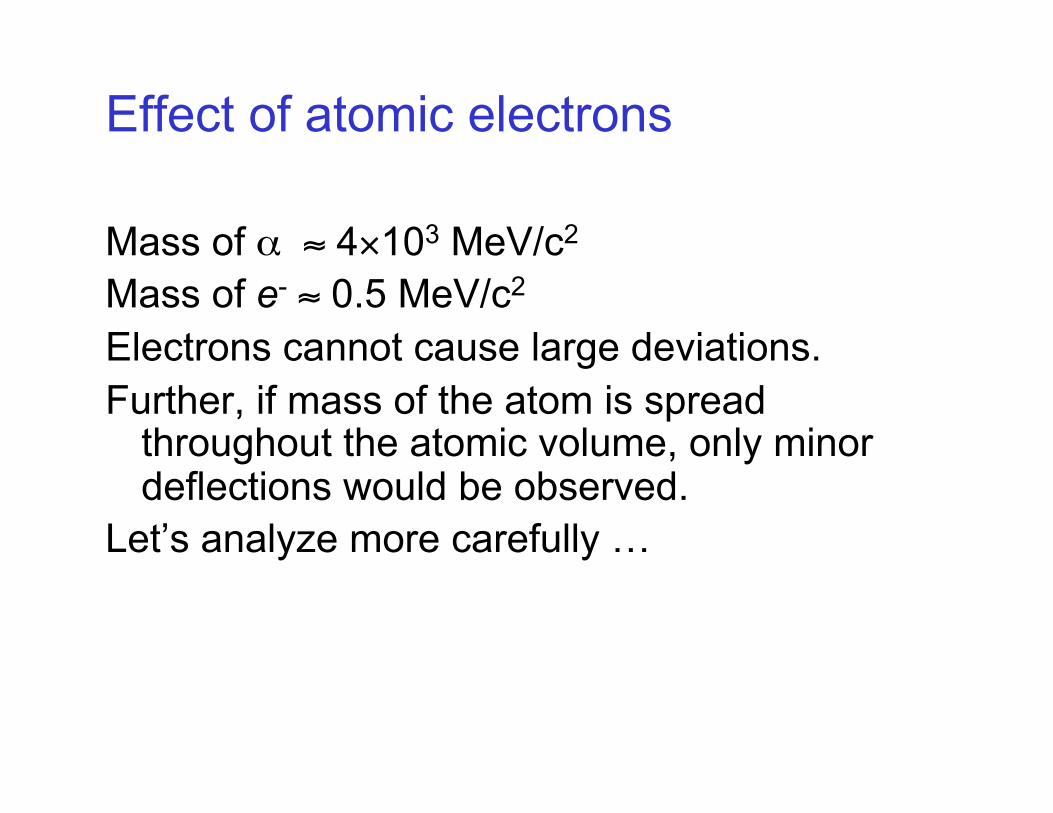
Effect of atomic electrons

Mass of α ≈ 4×103 MeV/c2

Mass of e- ≈ 0.5 MeV/c2 Electrons cannot cause large deviations. Further, if mass of the atom is spread

throughout the atomic volume, only minor deflections would be observed.

Let’s analyze more carefully …

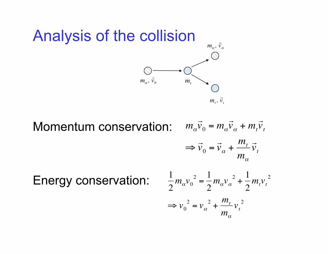
Analysis of the collision

Momentum conservation:

Energy conservation:

€

mα

v 0 = mα

v α + mt

v t

⇒ v 0 = v α +

mt

mα

v t

€

12mαv0

2 =12mαvα

2 +12mtvt

2

⇒ v02 = vα

2 +mt

mα

vt2

€

mα , v 0

€

mt

€

mt , v t

€

mα , v α

Analysis, cont’d.

Combining these equations, gives

  For mα >> mt, LHS > 0 and motion of α is along incident direction.

  For mα << mt, LHS < 0 and motion of α is along backward direction.

  For electrons as target, the first condition applies and hence backward scattering does not occur.

€

vt2 1− mt

mα

= 2 v α ⋅ v t

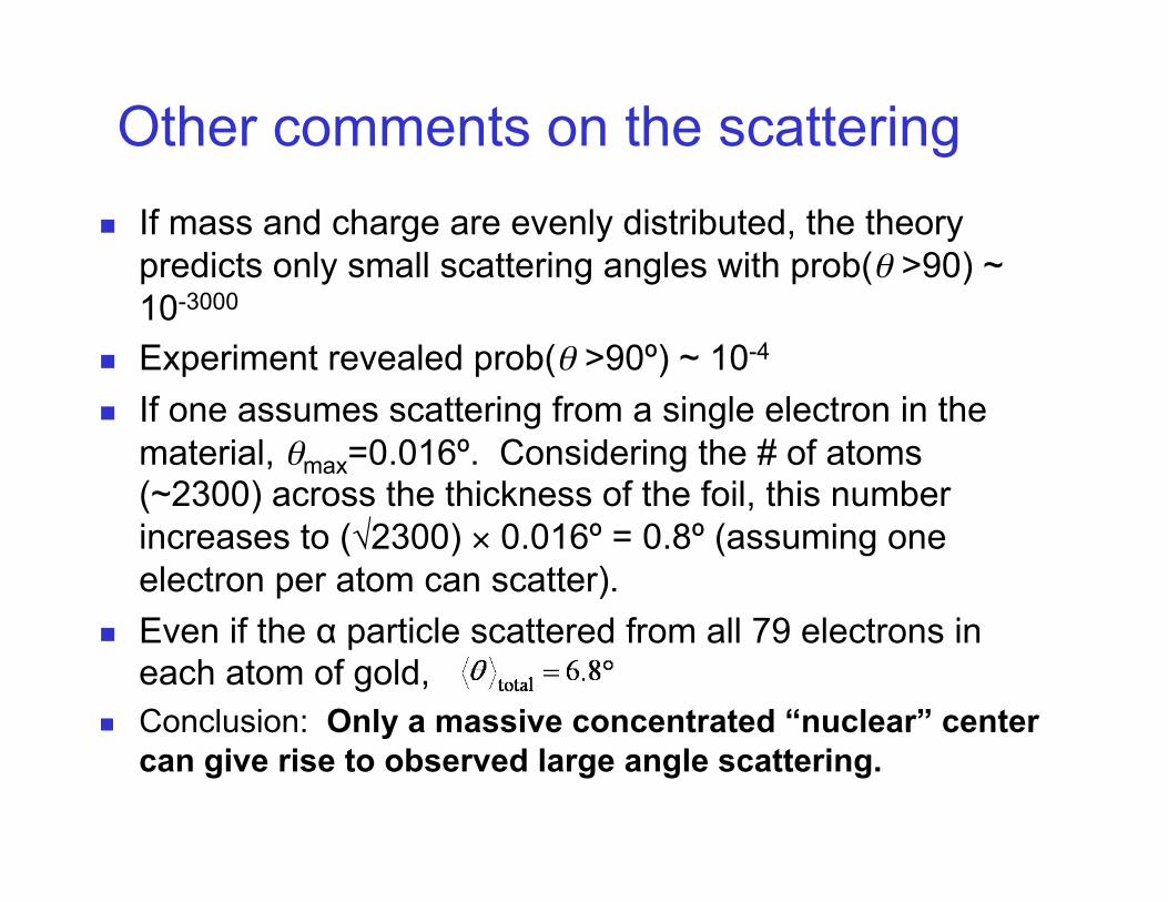
Other comments on the scattering   If mass and charge are evenly distributed, the theory

predicts only small scattering angles with prob(θ >90) ~ 10-3000

  Experiment revealed prob(θ >90º) ~ 10-4

  If one assumes scattering from a single electron in the material, θmax=0.016º. Considering the # of atoms (~2300) across the thickness of the foil, this number increases to (√2300) × 0.016º = 0.8º (assuming one electron per atom can scatter).

  Even if the α particle scattered from all 79 electrons in each atom of gold,

  Conclusion: Only a massive concentrated “nuclear” center can give rise to observed large angle scattering.

Coulomb Scattering

  Energy/Momentum conservation gives the correct asymptotic values for the particles involved in the scattering.

  To go further, we must consider the Coulomb force between the α and the atomic nucleus.

  Both are positively charged, so the force is repulsive.

  First, an aside on UNITS …

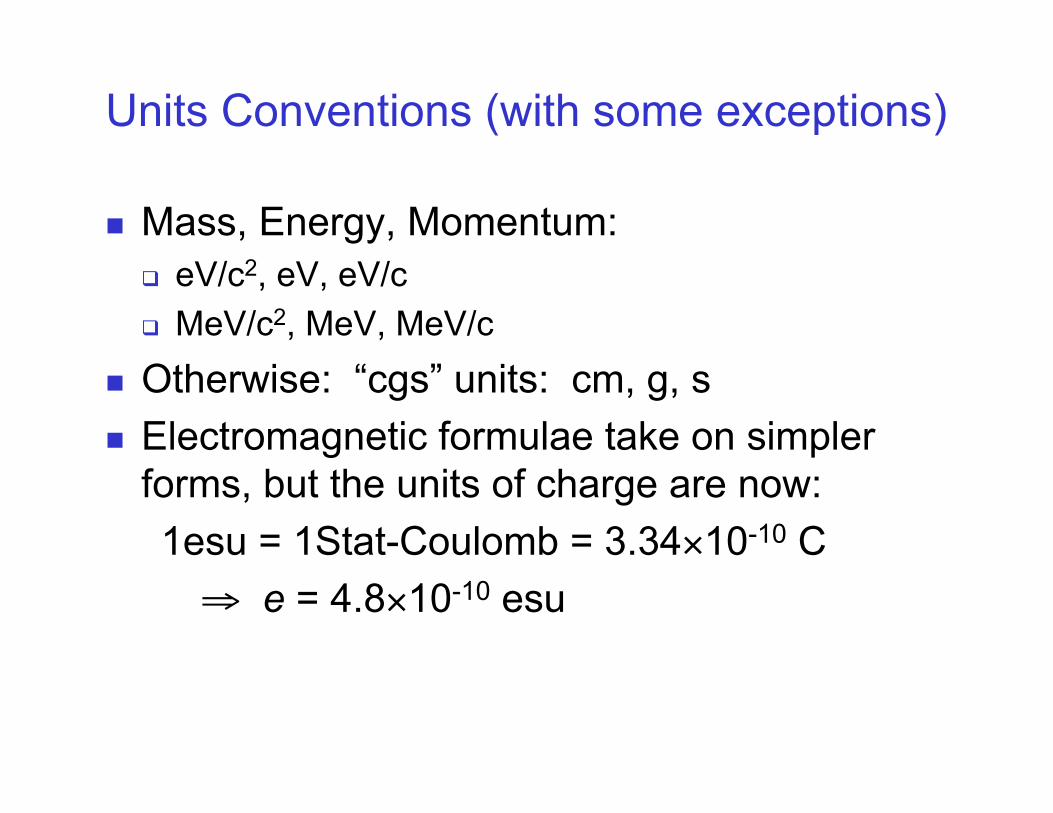
Units Conventions (with some exceptions)

  Mass, Energy, Momentum:   eV/c2, eV, eV/c   MeV/c2, MeV, MeV/c

  Otherwise: “cgs” units: cm, g, s   Electromagnetic formulae take on simpler

forms, but the units of charge are now: 1esu = 1Stat-Coulomb = 3.34×10-10 C ⇒ e = 4.8×10-10 esu

Coulomb Scattering Analysis

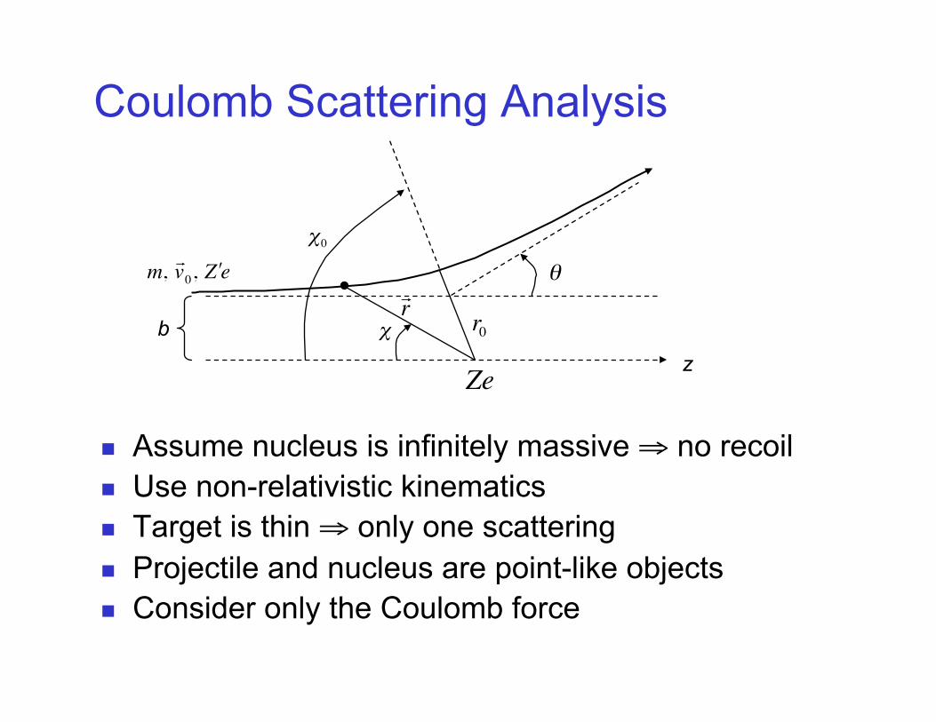
  Assume nucleus is infinitely massive ⇒ no recoil   Use non-relativistic kinematics   Target is thin ⇒ only one scattering   Projectile and nucleus are point-like objects   Consider only the Coulomb force

€

r

€

r0€

θ

z

b €

χ0

€

χ

€

m, v 0, ′ Z e

€

Ze

Scattering from a central potential V(r)

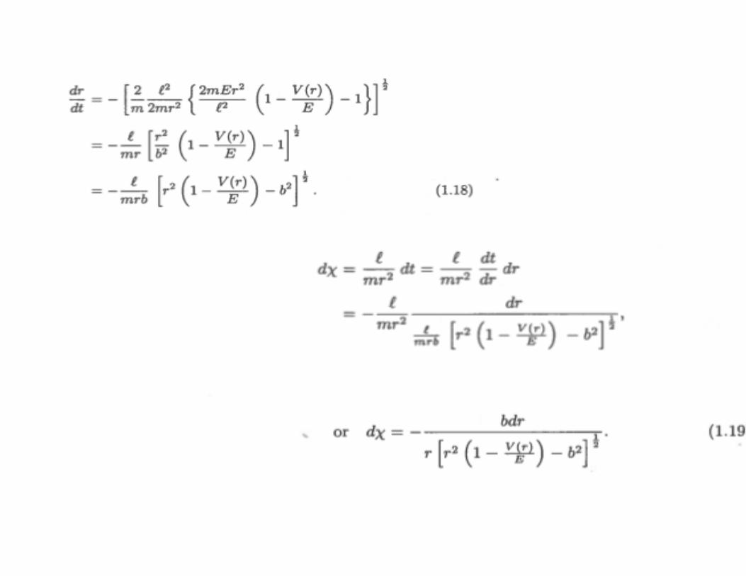
Scattering angle as a function of the impact parameter

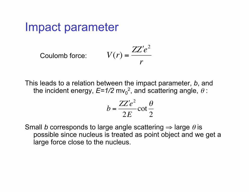
Impact parameter

Coulomb force:

This leads to a relation between the impact parameter, b, and the incident energy, E=1/2 mv0

2, and scattering angle, θ :

Small b corresponds to large angle scattering ⇒ large θ is possible since nucleus is treated as point object and we get a large force close to the nucleus.

€

V (r) =Z ′ Z e2

r

€

b =Z ′ Z e2

2Ecot θ

2

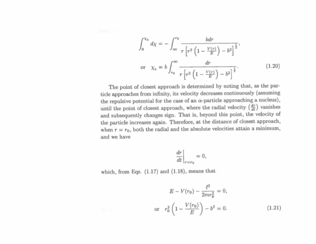
Distance of closest approach

  It can also be shown that the distance of closest approach, r0, is given by

  The previous slide shows that for non-zero θ, b→0 as E→∞. Therefore r0 →0 as E→∞.

  Thus, at high enough energy we can approach the nucleus as closely as we wish. The assumption of a point-like nucleus can then be tested.

€

r0 =Z ′ Z e2

2E1+ 1+

4b2E 2

Z ′ Z e2( )2

E→∞ → b

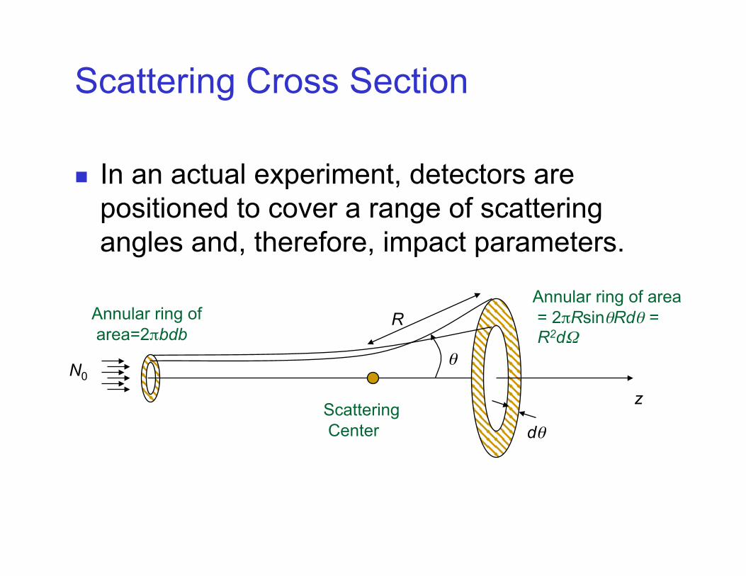
Scattering Cross Section

  In an actual experiment, detectors are positioned to cover a range of scattering angles and, therefore, impact parameters.

Scattering Center

Annular ring of area = 2πRsinθRdθ = R2dΩ

Annular ring of area=2πbdb

z

N0

R

θ

dθ

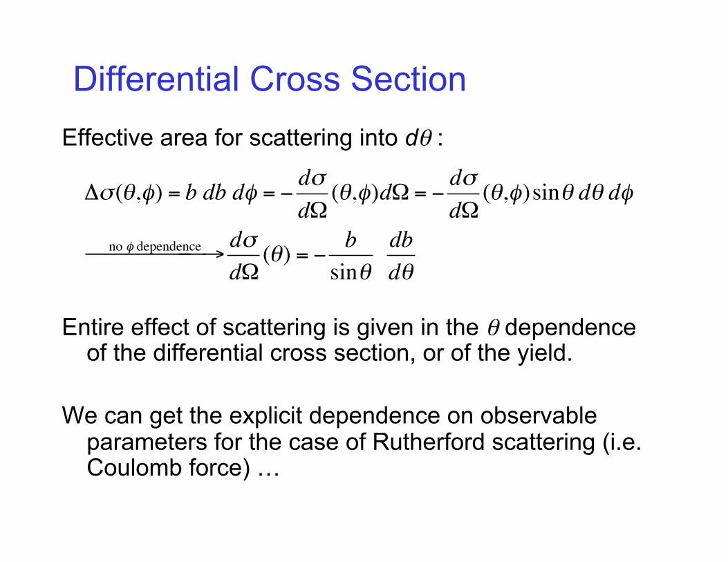
Differential Cross Section Effective area for scattering into dθ :

Entire effect of scattering is given in the θ dependence of the differential cross section, or of the yield.

We can get the explicit dependence on observable parameters for the case of Rutherford scattering (i.e. Coulomb force) …

€

Δσ (θ,φ) = b db dφ = −dσdΩ

(θ,φ)dΩ = −dσdΩ

(θ,φ)sinθ dθ dφ

no φ dependence → dσdΩ

(θ) = −b

sinθ dbdθ

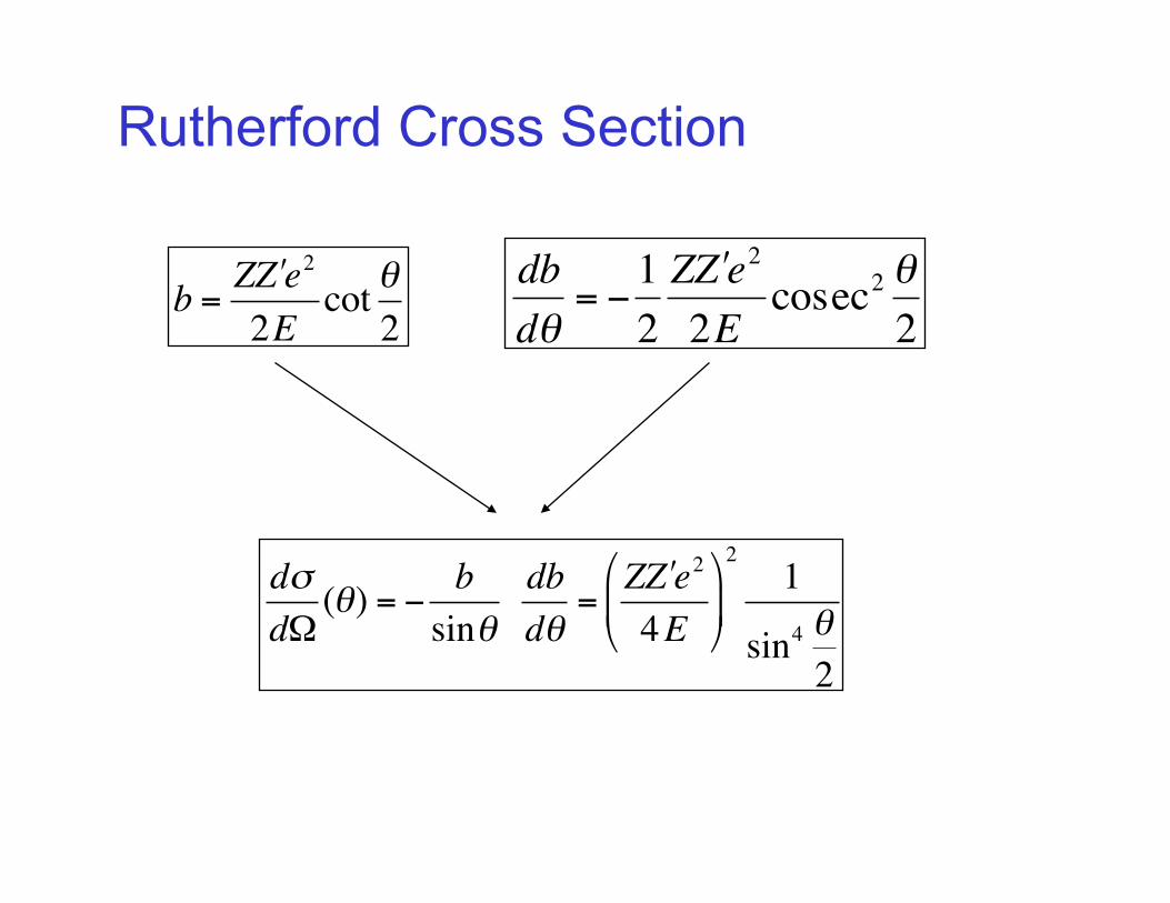
Rutherford Cross Section

€

b =Z ′ Z e2

2Ecot θ

2

€

dbdθ

= −12

Z ′ Z e2

2Ecosec2 θ

2

€

dσdΩ

(θ) = −b

sinθ db

dθ=

Z ′ Z e2

4E

21

sin4 θ2

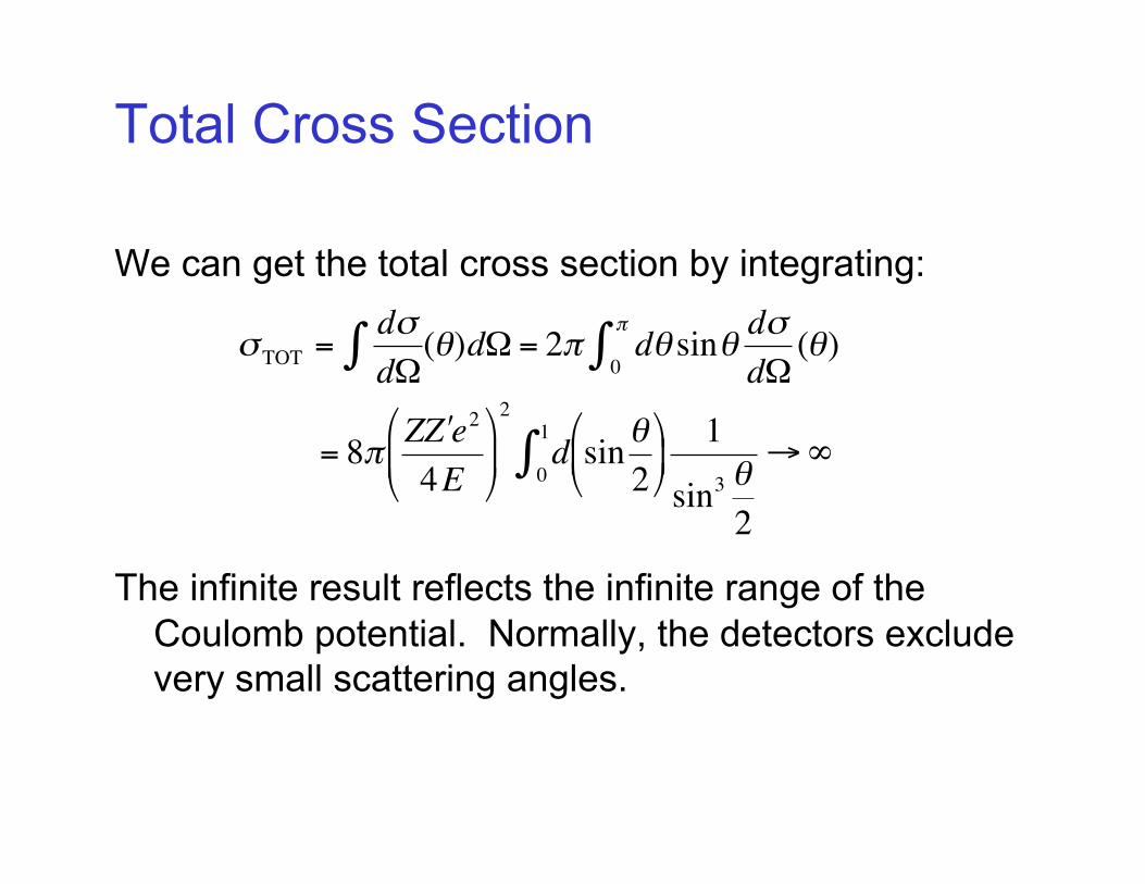
Total Cross Section

We can get the total cross section by integrating:

The infinite result reflects the infinite range of the Coulomb potential. Normally, the detectors exclude very small scattering angles. €

σTOT =dσdΩ∫ (θ)dΩ = 2π dθ sinθ

0

π

∫ dσdΩ

(θ)

= 8π Z ′ Z e2

4E

2

d sinθ2

0

1∫ 1

sin3 θ2

→∞

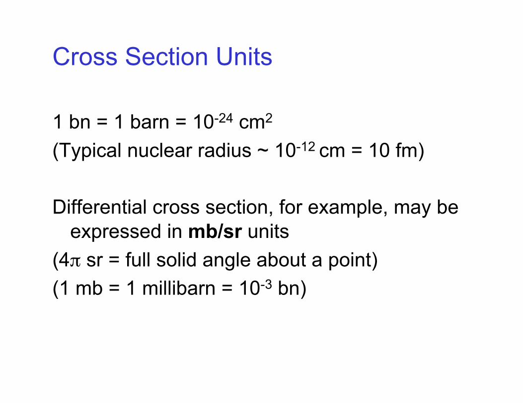
Cross Section Units

1 bn = 1 barn = 10-24 cm2

(Typical nuclear radius ~ 10-12 cm = 10 fm)

Differential cross section, for example, may be expressed in mb/sr units

(4π sr = full solid angle about a point) (1 mb = 1 millibarn = 10-3 bn)

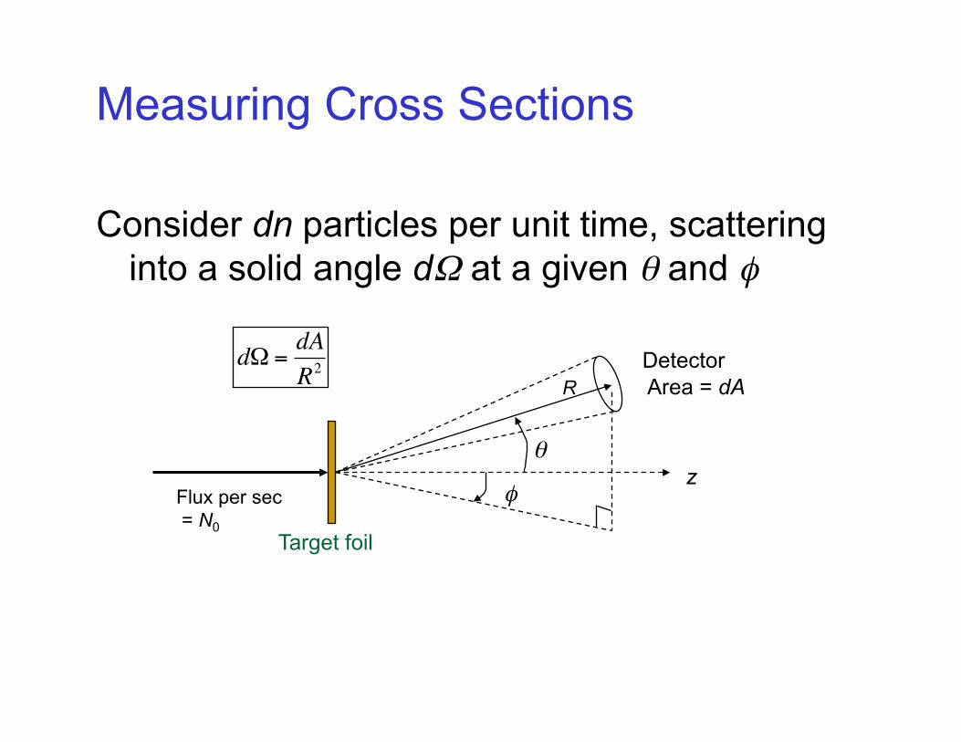
Measuring Cross Sections

Consider dn particles per unit time, scattering into a solid angle dΩ at a given θ and φ

RDetector Area = dA

z θ

φFlux per sec = N0

€

dΩ =dAR2

Target foil

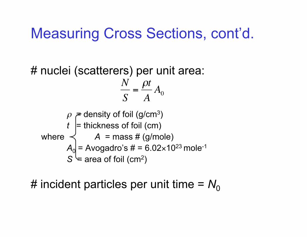
Measuring Cross Sections, cont’d.

# nuclei (scatterers) per unit area:

ρ = density of foil (g/cm3) t = thickness of foil (cm) where A = mass # (g/mole) A0 = Avogadro’s # = 6.02×1023 mole-1 S = area of foil (cm2)

# incident particles per unit time = N0

€

NS

=ρtAA0

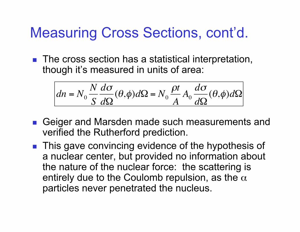
Measuring Cross Sections, cont’d.

  The cross section has a statistical interpretation, though it’s measured in units of area:

  Geiger and Marsden made such measurements and verified the Rutherford prediction.

  This gave convincing evidence of the hypothesis of a nuclear center, but provided no information about the nature of the nuclear force: the scattering is entirely due to the Coulomb repulsion, as the α particles never penetrated the nucleus.

€

dn = N0NSdσdΩ(θ,φ)dΩ = N0

ρtAA0dσdΩ(θ,φ)dΩ

Laboratory vs. CoM Frame

  We have ignored nuclear recoil, supposing that the mass of the target was infinite.

  We can treat this 2-body scattering problem in terms of relative and center-of-mass coordinates.

  The scattering can then be separated for central potentials:   The CoM moves at constant velocity.   The relative motion can be treated exactly as before,

except that the projectile mass is replaced by the “reduced mass”.

  This is especially useful in treating colliding beam experiments.

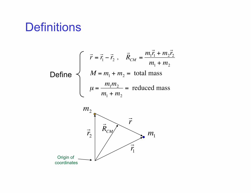
Definitions

€

r = r 1 − r 2 ,

R CM =

m1 r 1 + m2

r 2

m1 + m2

M = m1 + m2 = total mass

µ =m1m2

m1 + m2

= reduced mass

Define

€

r 1

€

r 2

€

r

€

R CM

€

m1€

m2

Origin of coordinates

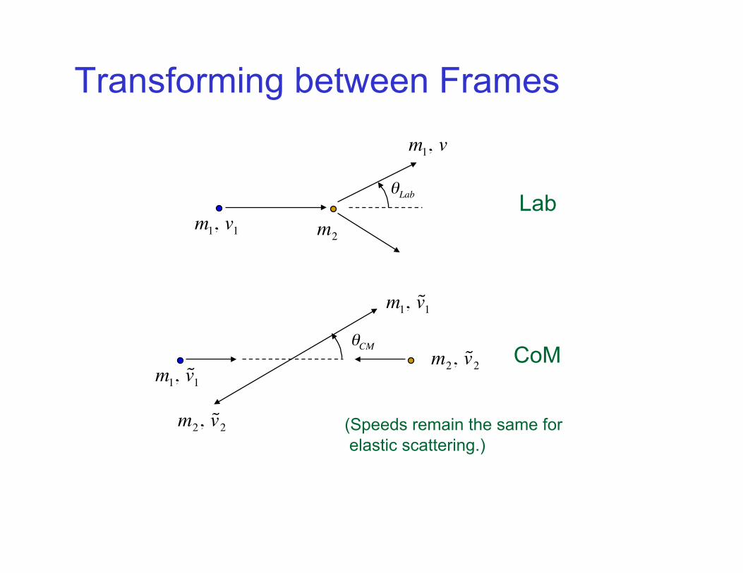
Transforming between Frames

€

m1, v1 €

m1, v

€

m2

€

θLab

€

m1, ˜ v 1€

θCM

€

m2, ˜ v 2

€

m1, ˜ v 1

€

m2, ˜ v 2

Lab

CoM

(Speeds remain the same for elastic scattering.)

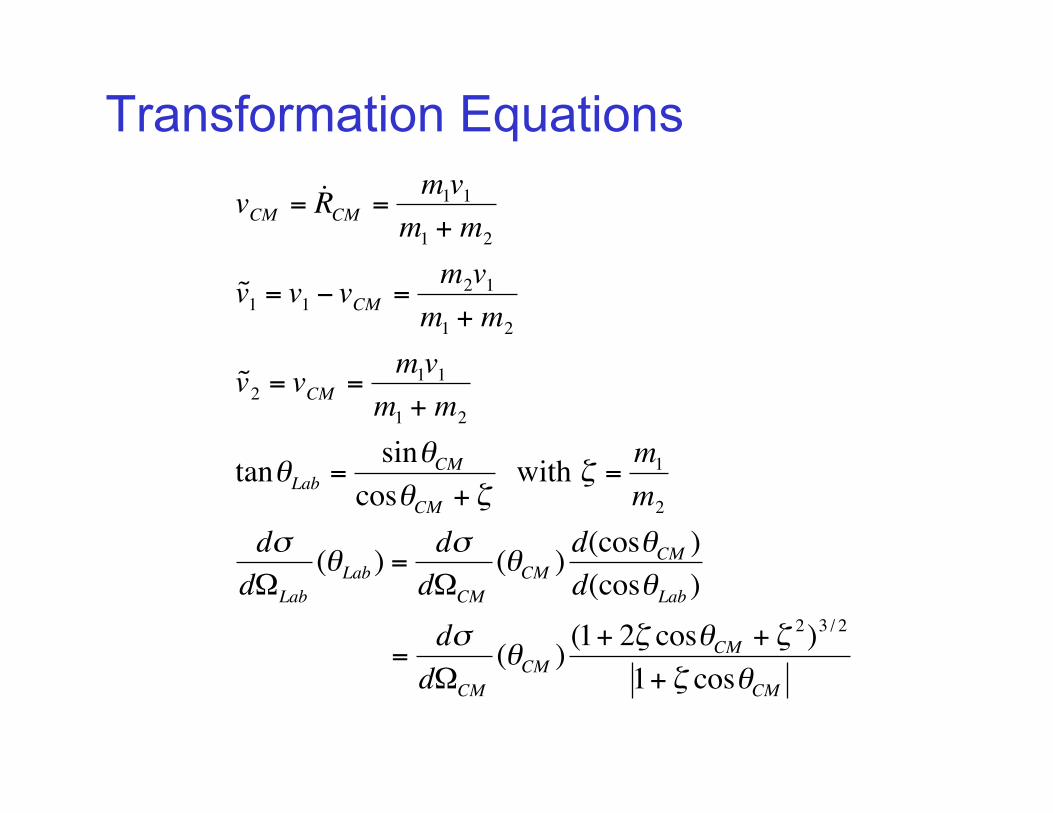
Transformation Equations

€

vCM = ˙ R CM =m1v1

m1 + m2

˜ v 1 = v1 − vCM =m2v1

m1 + m2

˜ v 2 = vCM =m1v1

m1 + m2

tanθLab =sinθCM

cosθCM + ζ with ζ =

m1

m2

dσdΩLab

(θLab ) =dσ

dΩCM

(θCM ) d(cosθCM )d(cosθLab )

=dσ

dΩCM

(θCM ) (1+ 2ζ cosθCM + ζ 2)3 / 2

1+ ζ cosθCM

Relativistic Variables

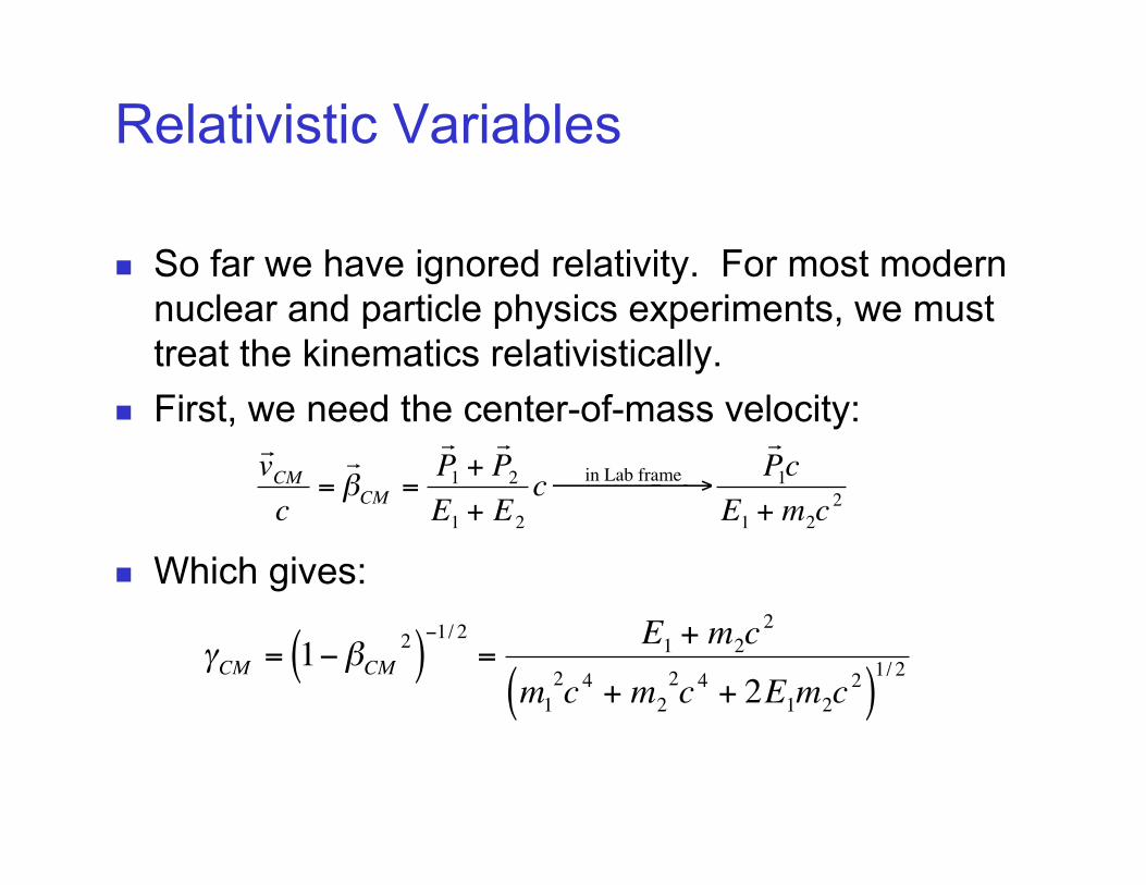
  So far we have ignored relativity. For most modern nuclear and particle physics experiments, we must treat the kinematics relativistically.

  First, we need the center-of-mass velocity:

  Which gives:

€

v CM

c= β CM =

P 1 + P 2

E1 + E2

c in Lab frame →

P 1c

E1 + m2c2

€

γCM = 1−βCM2( )

−1/ 2=

E1 + m2c2

m12c 4 + m2

2c 4 + 2E1m2c2( )1/ 2

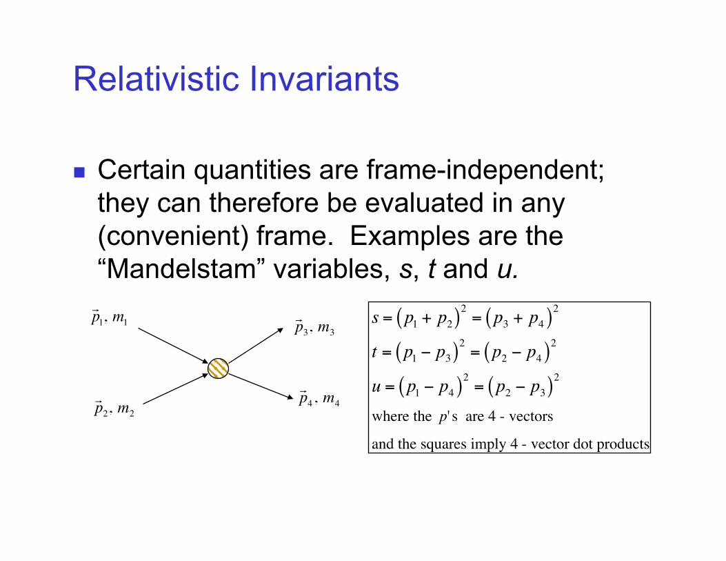
Relativistic Invariants

  Certain quantities are frame-independent; they can therefore be evaluated in any (convenient) frame. Examples are the “Mandelstam” variables, s, t and u.

€

p 1, m1

€

p 4, m4

€

p 3, m3

€

p 2, m2

€

s = p1 + p2( )2= p3 + p4( )2

t = p1 − p3( )2= p2 − p4( )2

u = p1 − p4( )2= p2 − p3( )2

where the p' s are 4 - vectors

and the squares imply 4 - vector dot products

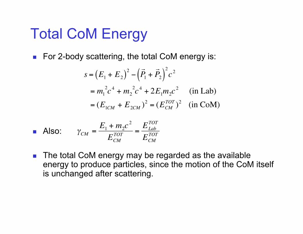
Total CoM Energy   For 2-body scattering, the total CoM energy is:

  Also:

  The total CoM energy may be regarded as the available energy to produce particles, since the motion of the CoM itself is unchanged after scattering.

€

s = E1 + E2( )2− P 1 + P 2( )

2c 2

= m12c 4 + m2

2c 4 + 2E1m2c2 (in Lab)

= (E1CM + E2CM )2 = (ECMTOT )2 (in CoM)

€

γCM =E1 + m2c

2

ECMTOT =

ELabTOT

ECMTOT

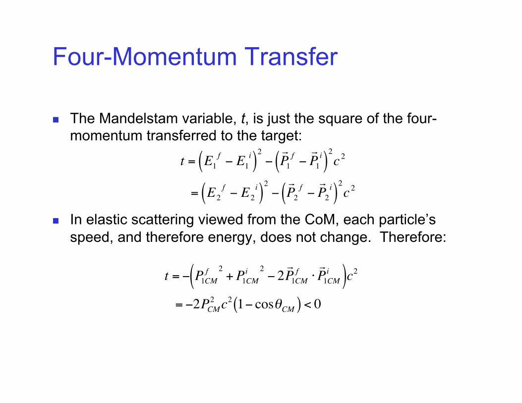
Four-Momentum Transfer

  The Mandelstam variable, t, is just the square of the four-momentum transferred to the target:

  In elastic scattering viewed from the CoM, each particle’s speed, and therefore energy, does not change. Therefore:

€

t = E1f − E1

i( )2− P 1

f − P 1

i( )2c 2

= E2f − E2

i( )2− P 2

f − P 2

i( )2c 2

€

t = − P1CMf 2

+ P1CMi 2

− 2 P 1CM

f ⋅ P 1CM

i( )c2

= −2PCM2 c2 1− cosθCM( ) < 0

Feynman Diagrams

  From the definition of t, we can consider the scattering to take place by the exchange of a particle, of mass m, where t = m2.

  Since t < 0, the particle has an imaginary rest mass and is therefore called virtual.

  Feynman invented pictorial representations of scattering processes, in which each picture has a precise mathematical meaning: a Feynman diagram.

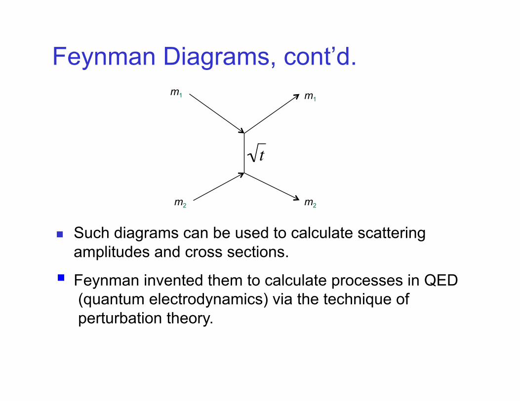
Feynman Diagrams, cont’d. m1

m2

m1

m2

€

t

  Such diagrams can be used to calculate scattering amplitudes and cross sections.

  Feynman invented them to calculate processes in QED (quantum electrodynamics) via the technique of perturbation theory.

Interpretation of Four-momentum Transfer

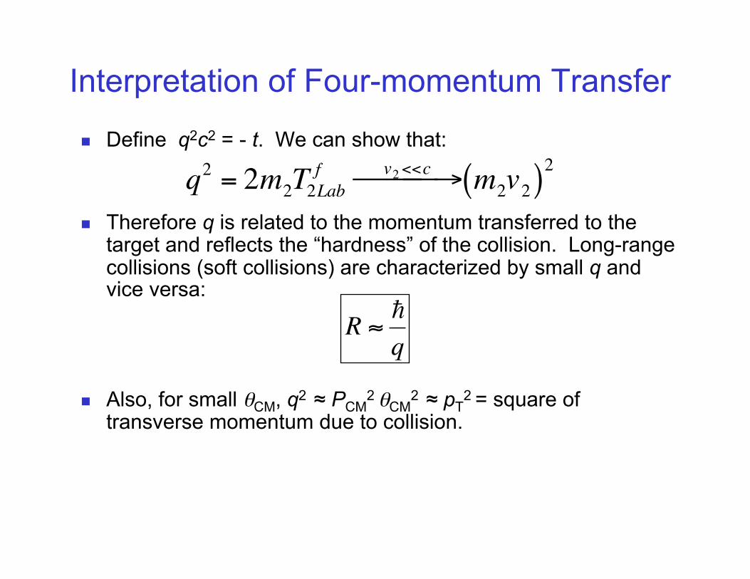
  Define q2c2 = - t. We can show that:

  Therefore q is related to the momentum transferred to the target and reflects the “hardness” of the collision. Long-range collisions (soft collisions) are characterized by small q and vice versa:

  Also, for small θCM, q2 ≈ PCM2 θCM

2 ≈ pT2 = square of

transverse momentum due to collision.

€

q2 = 2m2T2Labf v2<<c → m2v2( )2

€

R ≈ q

Back to Rutherford Scattering

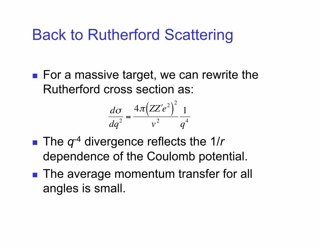
  For a massive target, we can rewrite the Rutherford cross section as:

  The q-4 divergence reflects the 1/r dependence of the Coulomb potential.

  The average momentum transfer for all angles is small.

€

dσdq2

=4π Z ′ Z e2( )

2

v 21q4

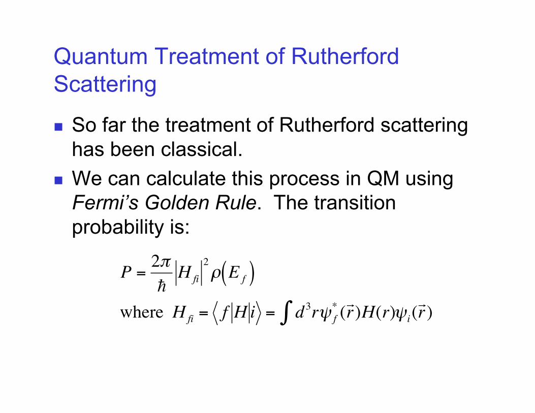
Quantum Treatment of Rutherford Scattering

  So far the treatment of Rutherford scattering has been classical.

  We can calculate this process in QM using Fermi’s Golden Rule. The transition probability is:

€

P =2π

H fi2ρ E f( )

where H fi = f H i = d3rψ f*∫ ( r )H(r)ψi(

r )

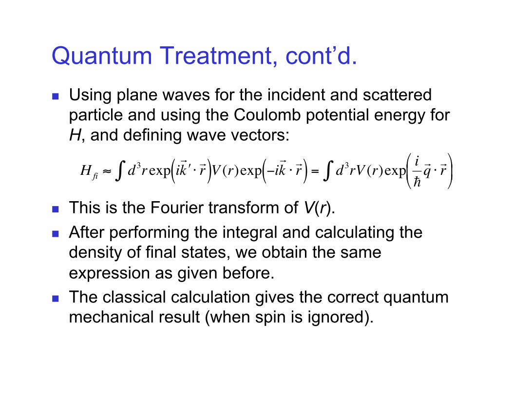
Quantum Treatment, cont’d.   Using plane waves for the incident and scattered

particle and using the Coulomb potential energy for H, and defining wave vectors:

  This is the Fourier transform of V(r).   After performing the integral and calculating the

density of final states, we obtain the same expression as given before.

  The classical calculation gives the correct quantum mechanical result (when spin is ignored).

€

H fi ≈ d3∫ rexp i ′ k ⋅ r ( )V (r)exp −i

k ⋅ r ( ) = d3∫ rV (r)exp i

q ⋅ r