Lecture Notes 7, Math/Comp 128, Math 250

Misha KilmerTufts University

October 23, 2005

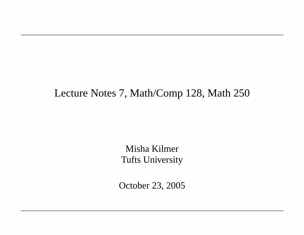
Floating Point Arithmetic

We talked last time about how the computer represents float-

ing point numbers.

• In a floating point number system, the numbers are not

equidistant.

• x = ±0.d1d2 . . . dt) × βe wheret is precision, β is the base,

e is the exponent,d1d2 . . . dt is the mantissa.

•System can usechoppingor rounding.

1

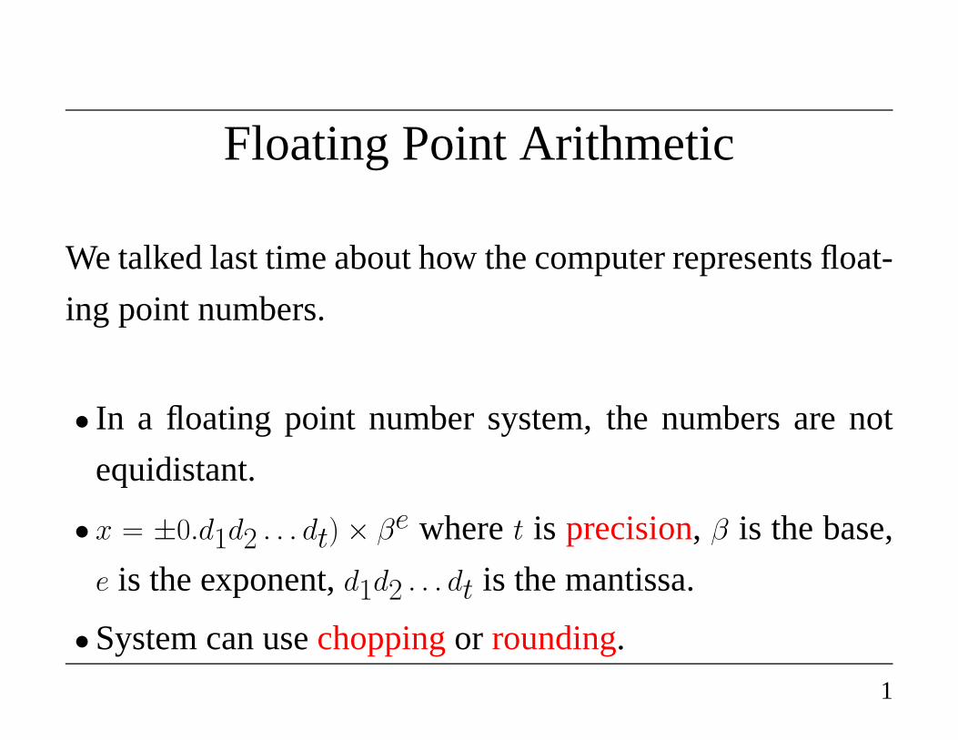
Chopping vs. Rounding

A method of convertingx ∈ R to fl(x) in F.

Chopping: ignore all digits aftertth digit

Rounding:fl(x) rounds up ift + 1st digit is≥ 1/2β and down

otherwise.

2

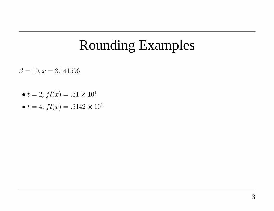
Rounding Examples

β = 10, x = 3.141596

• t = 2, fl(x) = .31 × 101

• t = 4, fl(x) = .3142 × 101

3

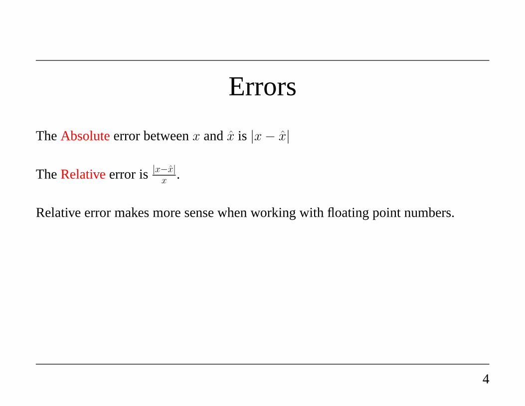
Errors

TheAbsoluteerror betweenx andx̂ is |x − x̂|

TheRelativeerror is |x−x̂|x .

Relative error makes more sense when working with floating point numbers.

4

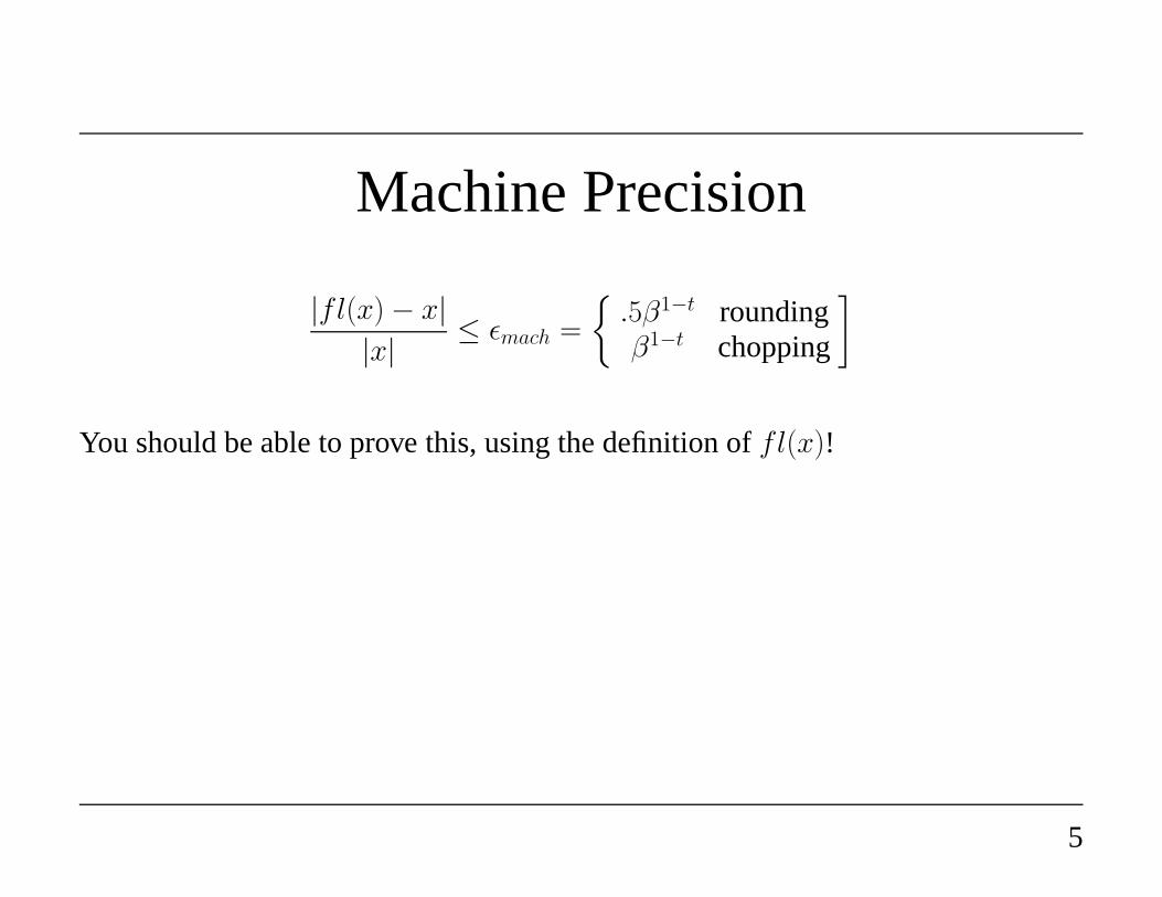
Machine Precision

|fl(x) − x|

|x|≤ εmach =

{

.5β1−t roundingβ1−t chopping

]

You should be able to prove this, using the definition offl(x)!

5

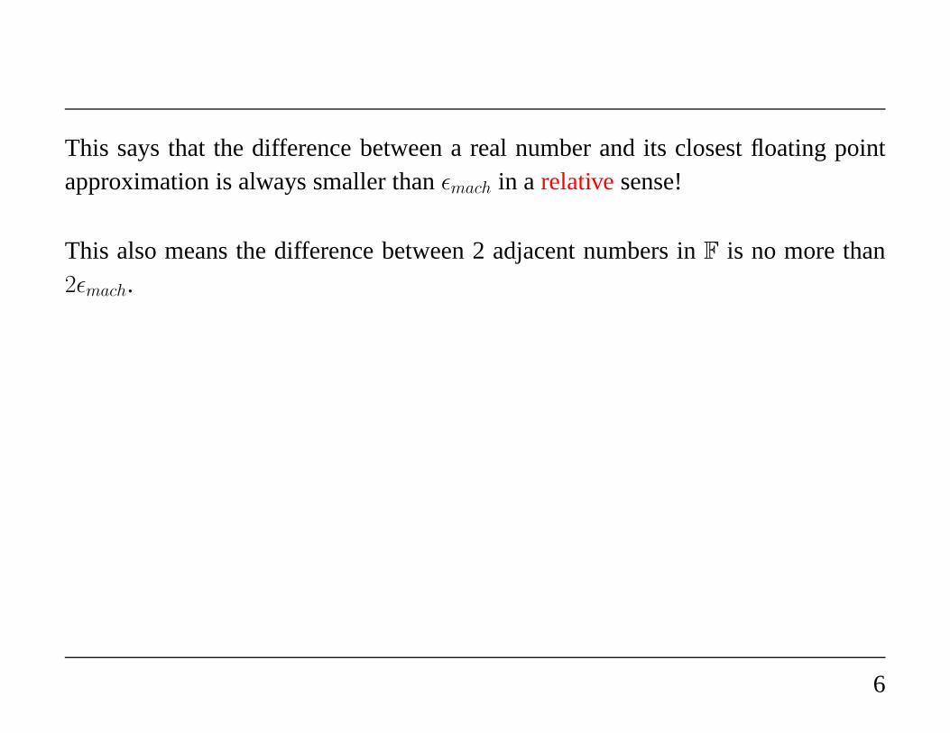
This says that the difference between a real number and its closest floating pointapproximation is always smaller thanεmach in a relativesense!

This also means the difference between 2 adjacent numbers inF is no more than2εmach.

6

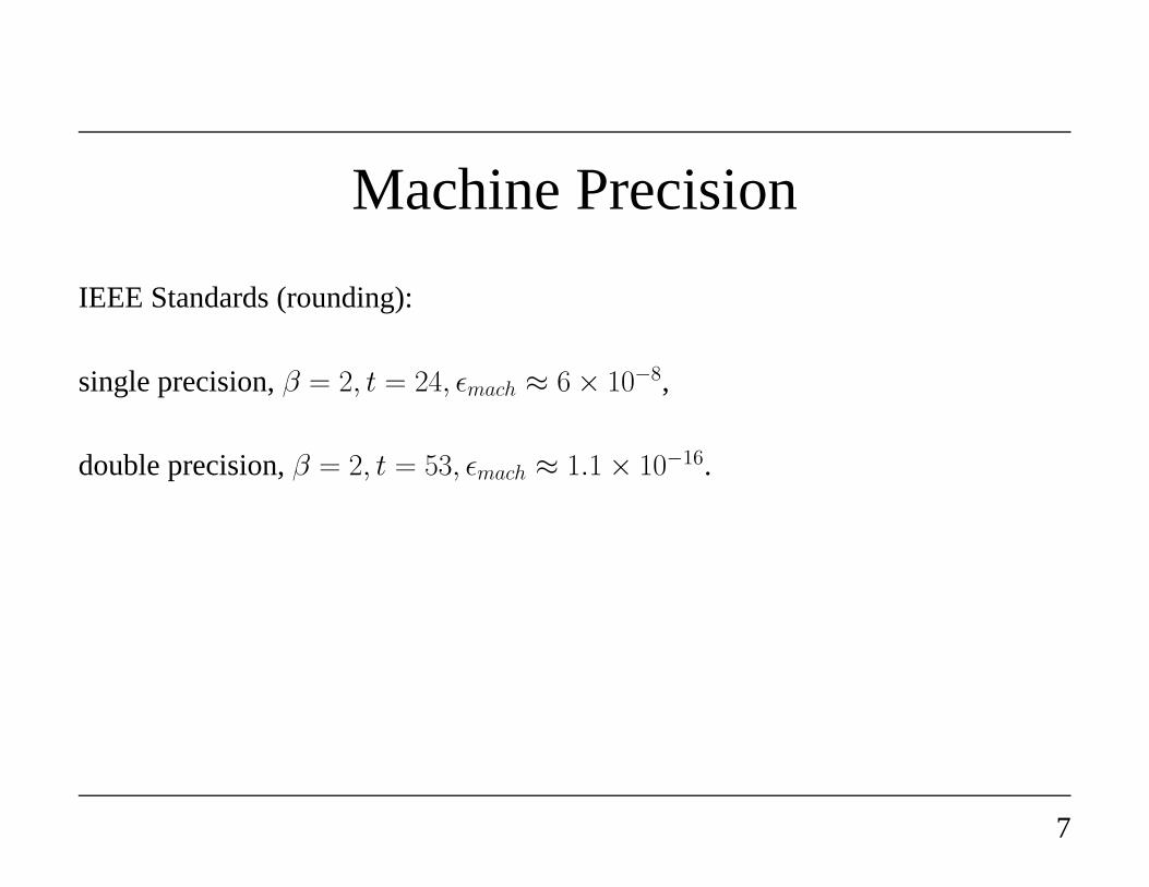
Machine Precision

IEEE Standards (rounding):

single precision,β = 2, t = 24, εmach ≈ 6 × 10−8,

double precision,β = 2, t = 53, εmach ≈ 1.1 × 10−16.

7

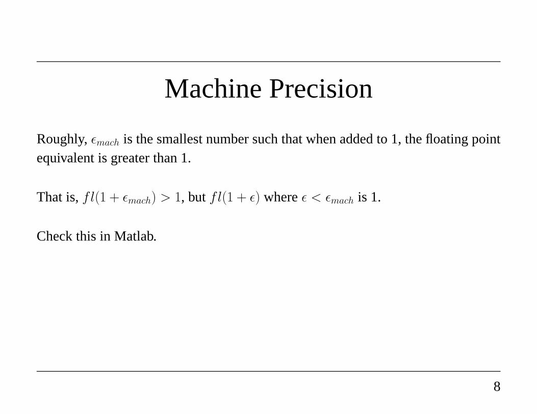
Machine Precision

Roughly,εmach is the smallest number such that when added to 1, the floating pointequivalent is greater than 1.

That is,fl(1 + εmach) > 1, butfl(1 + ε) whereε < εmach is 1.

Check this in Matlab.

8

Adding 2 numbers

If x, y ∈ R, x + y gets computed asfl(x) ⊕ fl(y).

Similar for other arithmetic operations.

9

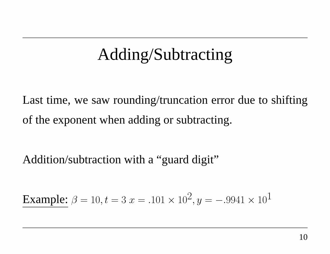
Adding/Subtracting

Last time, we saw rounding/truncation error due to shifting

of the exponent when adding or subtracting.

Addition/subtraction with a “guard digit”

Example:β = 10, t = 3 x = .101 × 102, y = −.9941 × 101

10

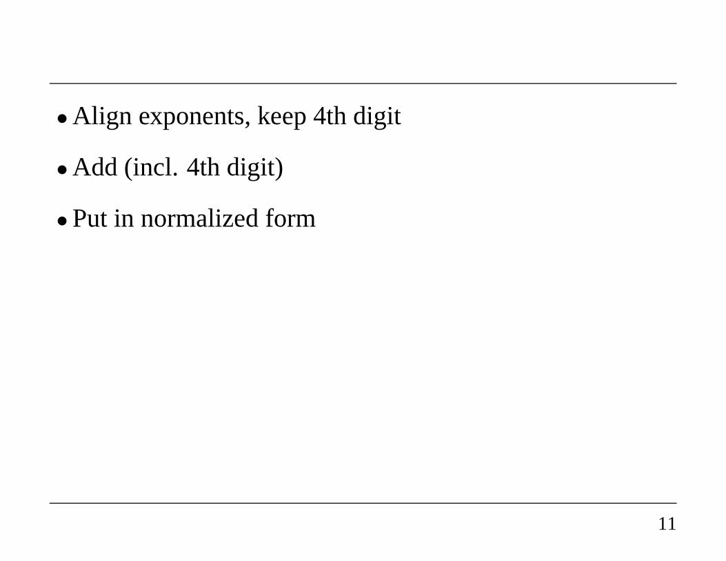
•Align exponents, keep 4th digit

•Add (incl. 4th digit)

•Put in normalized form

11

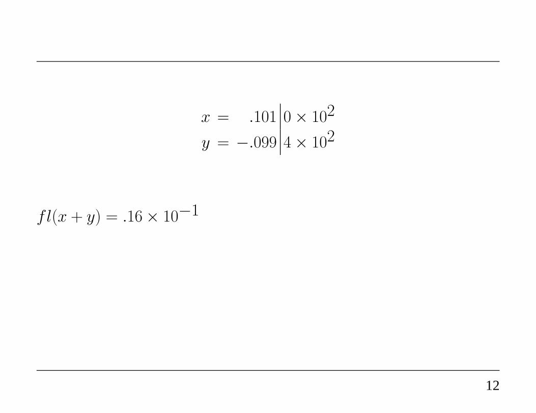
x = .101 0 × 102

y = −.099 4 × 102

fl(x + y) = .16 × 10−1

12

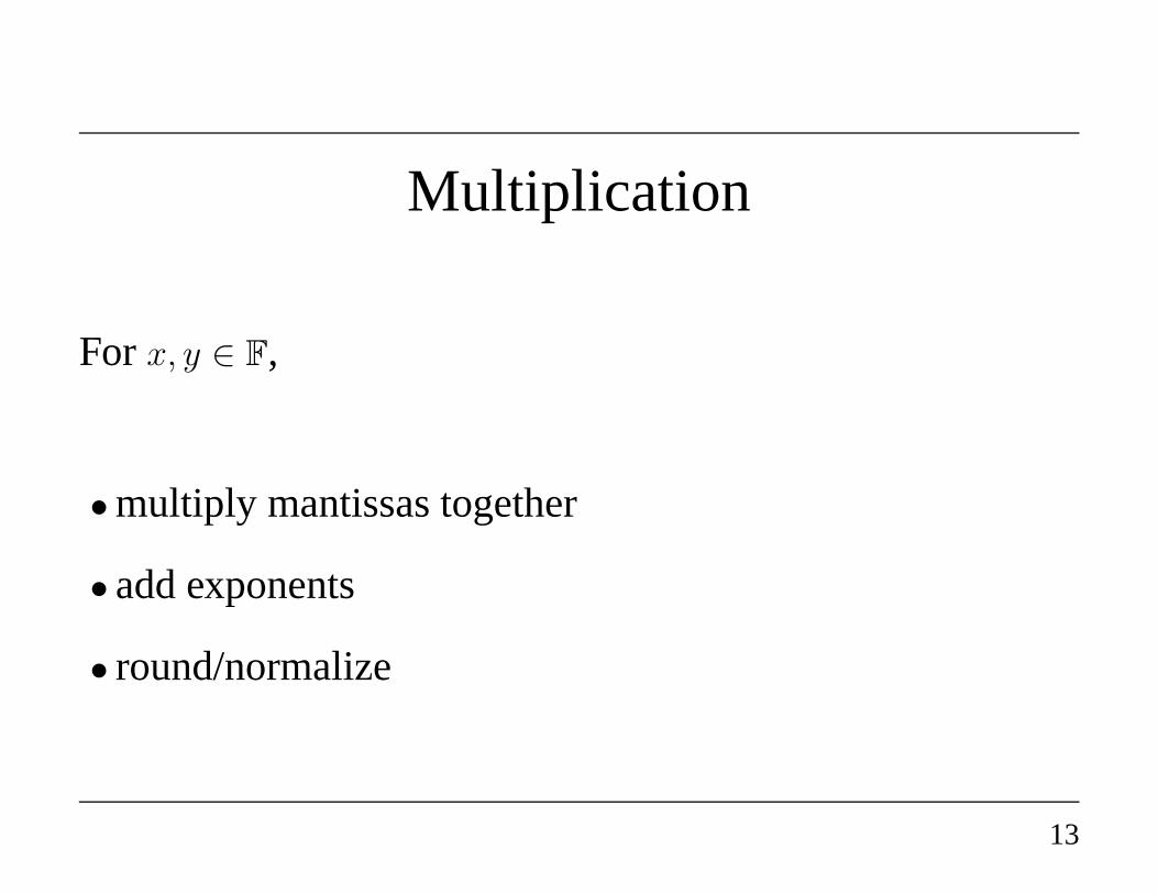
Multiplication

Forx, y ∈ F,

•multiply mantissas together

• add exponents

• round/normalize

13

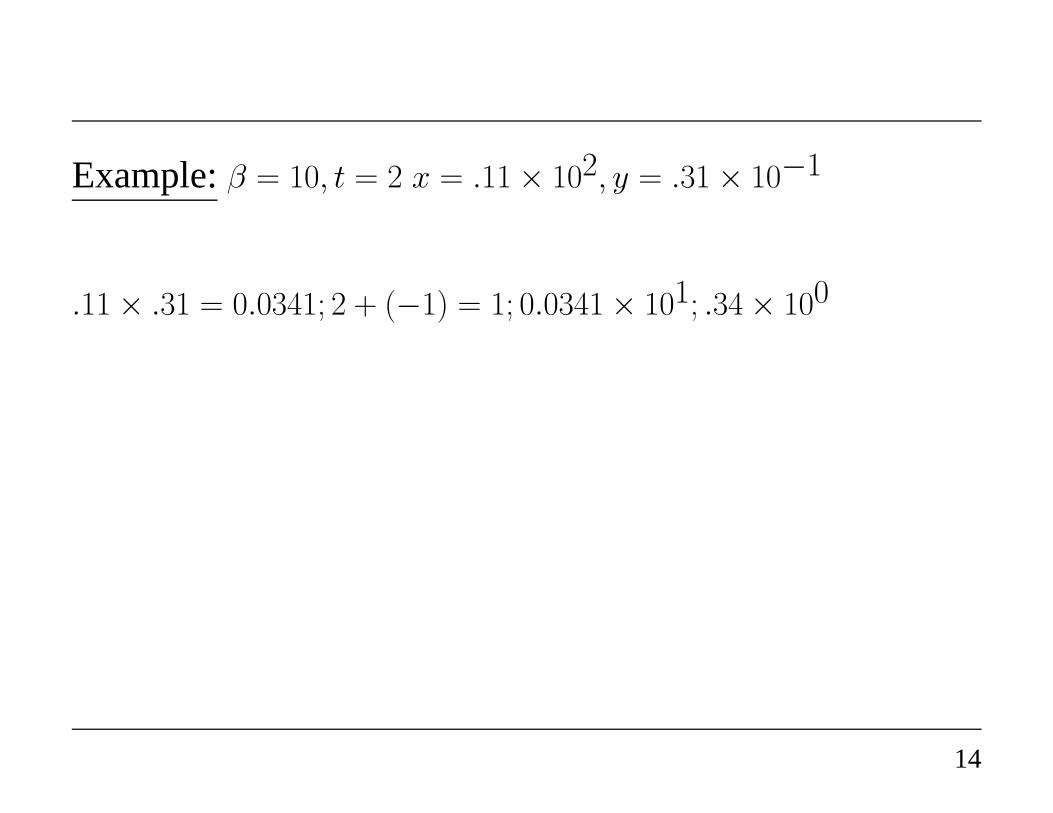
Example:β = 10, t = 2 x = .11 × 102, y = .31 × 10−1

.11 × .31 = 0.0341; 2 + (−1) = 1; 0.0341 × 101; .34 × 100

14

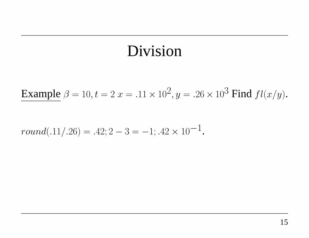
Division

Exampleβ = 10, t = 2 x = .11× 102, y = .26× 103 Find fl(x/y).

round(.11/.26) = .42; 2 − 3 = −1; .42 × 10−1.

15

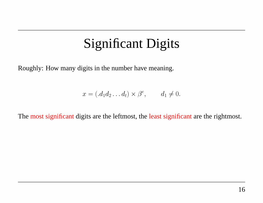
Significant Digits

Roughly: How many digits in the number have meaning.

x = (.d1d2 . . . dt) × βe, d1 6= 0.

Themost significantdigits are the leftmost, theleast significantare the rightmost.

16

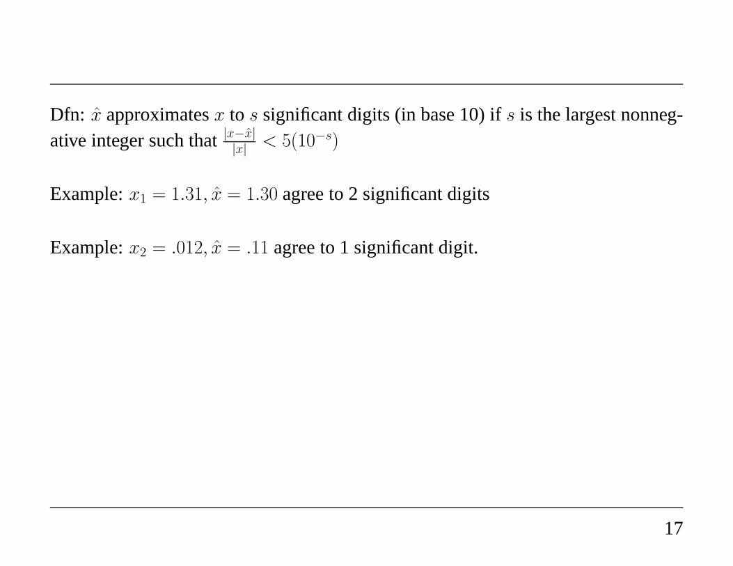
Dfn: x̂ approximatesx to s significant digits (in base 10) ifs is the largest nonneg-ative integer such that|x−x̂|

|x| < 5(10−s)

Example:x1 = 1.31, x̂ = 1.30 agree to 2 significant digits

Example:x2 = .012, x̂ = .11 agree to 1 significant digit.

17

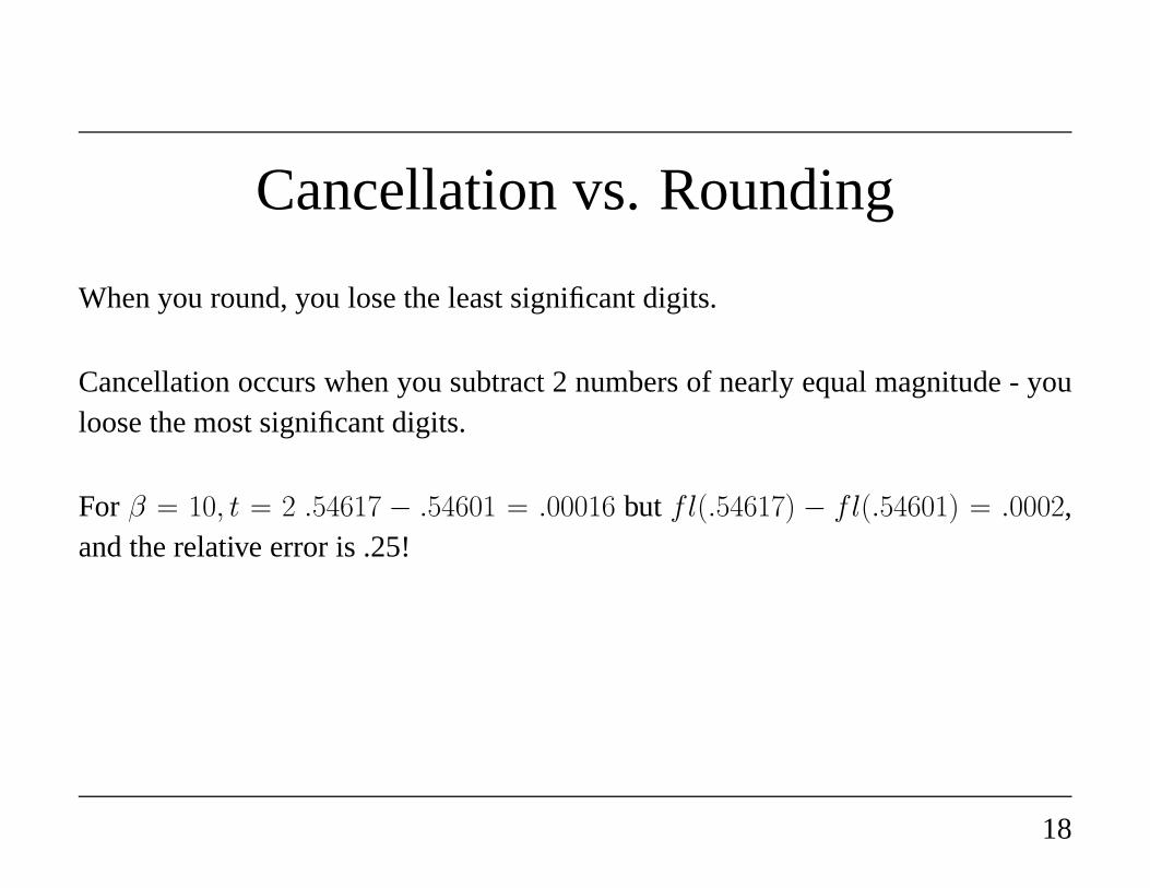
Cancellation vs. Rounding

When you round, you lose the least significant digits.

Cancellation occurs when you subtract 2 numbers of nearly equal magnitude - youloose the most significant digits.

For β = 10, t = 2 .54617 − .54601 = .00016 but fl(.54617) − fl(.54601) = .0002,and the relative error is .25!

18

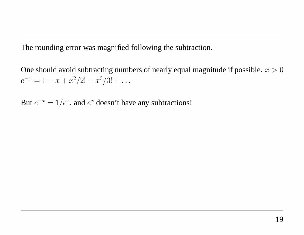
The rounding error was magnified following the subtraction.

One should avoid subtracting numbers of nearly equal magnitude if possible.x > 0

e−x = 1 − x + x2/2! − x3/3! + . . .

But e−x = 1/ex, andex doesn’t have any subtractions!

19

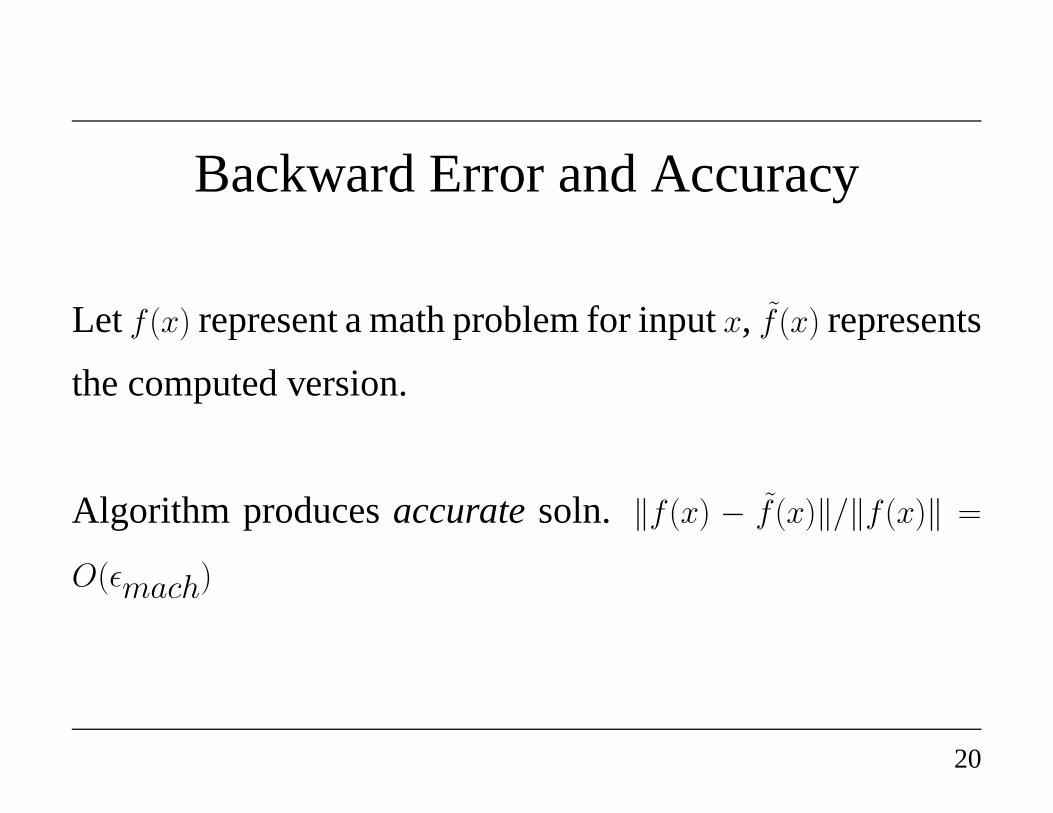
Backward Error and Accuracy

Let f (x) represent a math problem for inputx, f̃ (x) represents

the computed version.

Algorithm producesaccurate soln. ‖f (x) − f̃(x)‖/‖f (x)‖ =

O(εmach)

20

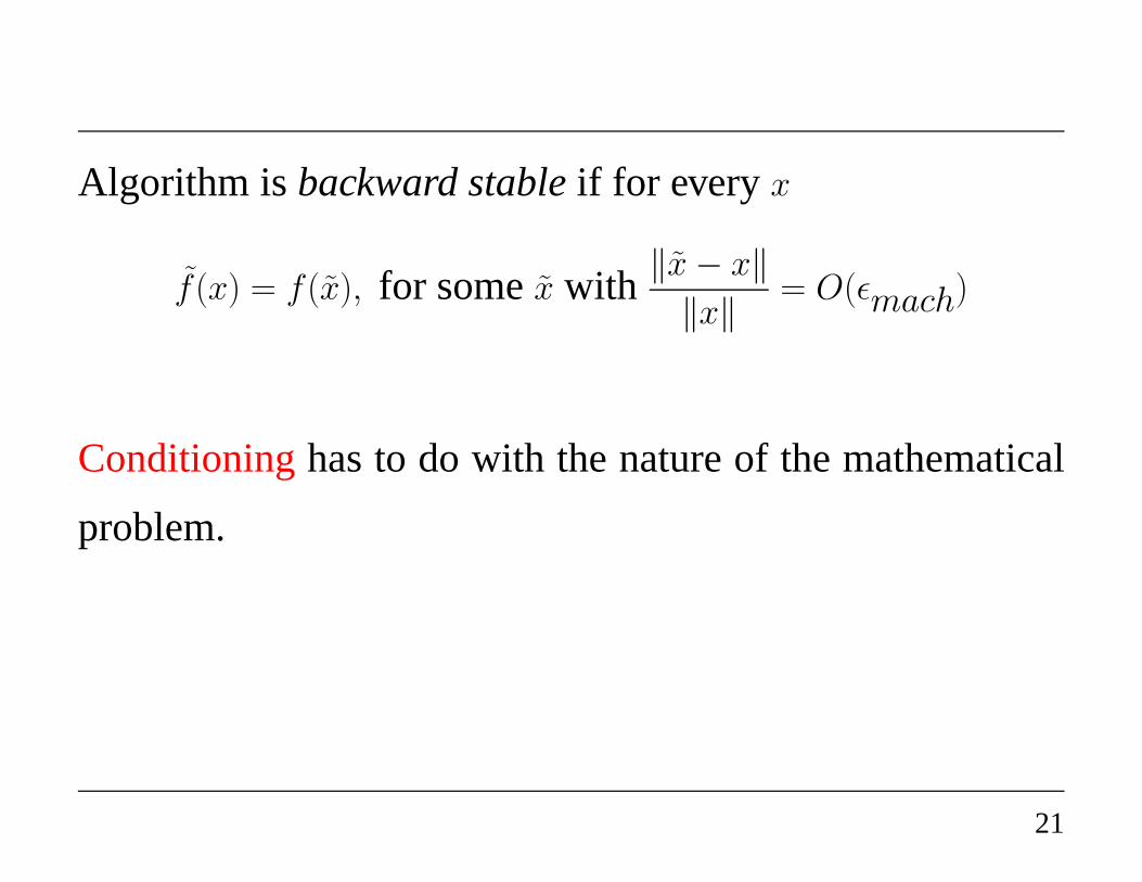
Algorithm is backward stable if for everyx

f̃ (x) = f (x̃), for somex̃ with‖x̃ − x‖

‖x‖= O(εmach)

Conditioninghas to do with the nature of the mathematical

problem.

21

Conditioning vs. Stability

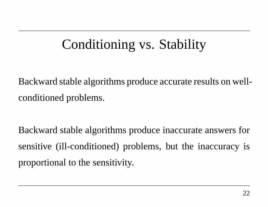
Backward stable algorithms produce accurate results on well-

conditioned problems.

Backward stable algorithms produce inaccurate answers for

sensitive (ill-conditioned) problems, but the inaccuracyis

proportional to the sensitivity.

22

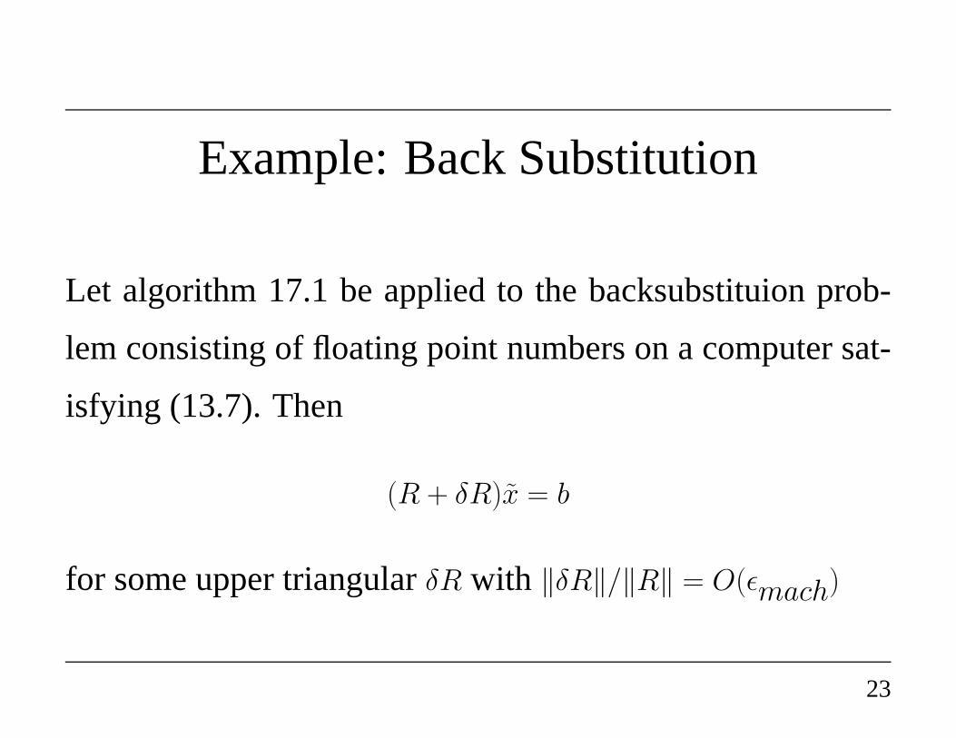
Example: Back Substitution

Let algorithm 17.1 be applied to the backsubstituion prob-

lem consisting of floating point numbers on a computer sat-

isfying (13.7). Then

(R + δR)x̃ = b

for some upper triangularδR with ‖δR‖/‖R‖ = O(εmach)

23

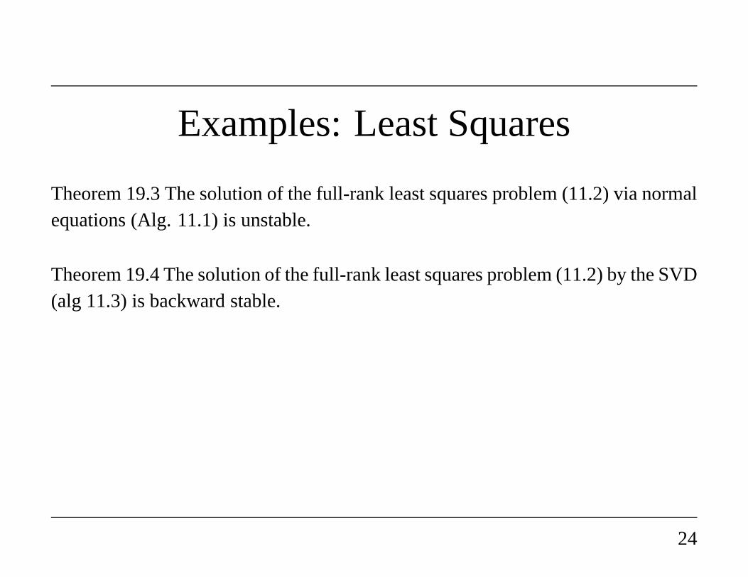
Examples: Least Squares

Theorem 19.3 The solution of the full-rank least squares problem (11.2) via normalequations (Alg. 11.1) is unstable.

Theorem 19.4 The solution of the full-rank least squares problem (11.2) by the SVD(alg 11.3) is backward stable.

24

Backward Stable Algorithms

We concentrate on designing backward stable algorithms!

25