lecture notes 15 tuesday, march 2nd, 2010biomechanics.stanford.edu/me338_10/me338_n15.pdflecture...
26
ME338A CONTINUUM MECHANICS lecture notes 15 tuesday, march 2nd, 2010
Transcript of lecture notes 15 tuesday, march 2nd, 2010biomechanics.stanford.edu/me338_10/me338_n15.pdflecture...
ME338ACONTINUUM MECHANICS
lecture notes 15
tuesday, march 2nd, 2010
5 Introduction to NonlinearContinuum Mechanics
5.1 Kinematics
5.1.1 Motion and Configurations
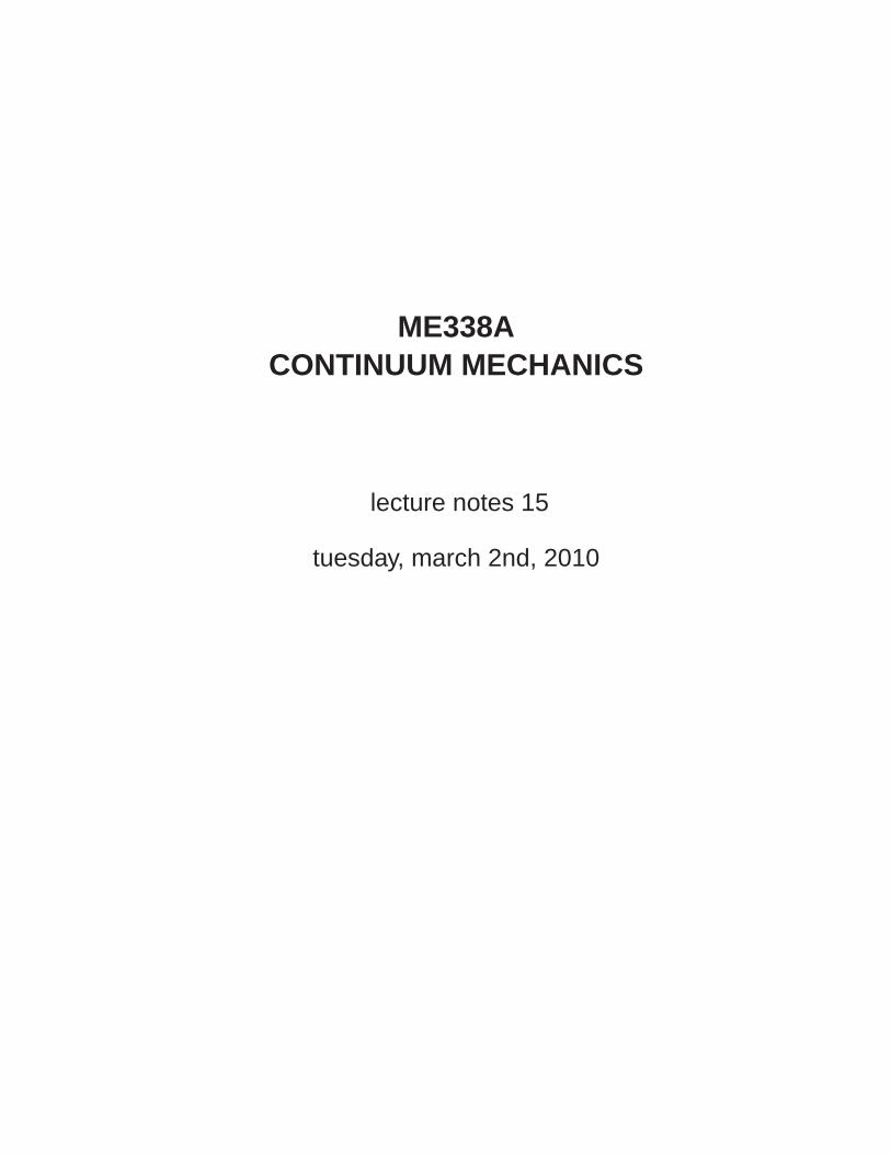
Consider a material body B composed of infinitely many ma-
terial points P ∈ B that are identified with geometrical points
in the three-dimensional Euclidean space R3.
R3
P
B
xt
Bt
χt(P)
e1
e2
e3
The configuration of the body B in R3 at time t is described
by the one-to-one relation
χt :
B → Bt ∈ R3 ,
P ∈ B 7→ xt = χt(P) ∈ Bt .(5.1.1)
Having this definition at hand, we go on to describe the mo-
tion of the body as a family of configurations parameterized
125
5 Introduction to Nonlinear Continuum Mechanics
R3
P
B
Path
χt0(P)
χt1(P)
χt2(P)
χt3(P)
χt4(P)
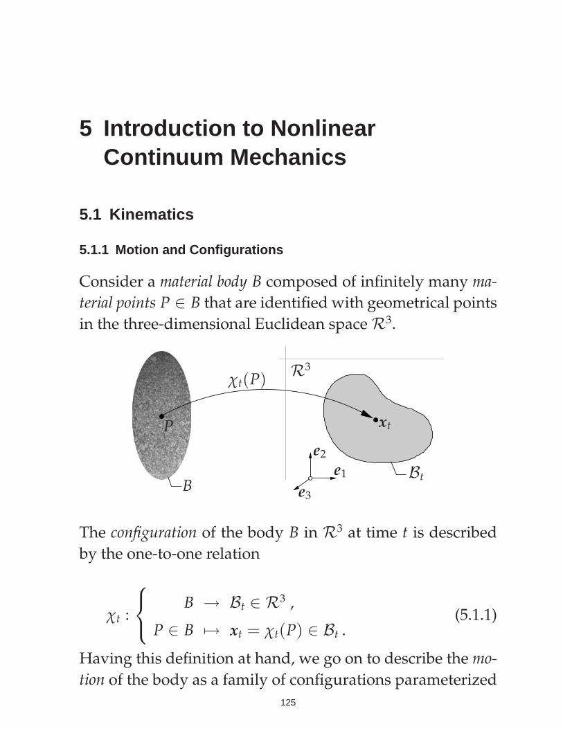
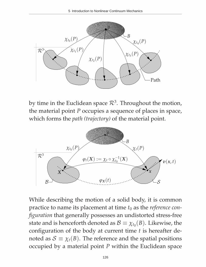
by time in the Euclidean space R3. Throughout the motion,
the material point P occupies a sequence of places in space,
which forms the path (trajectory) of the material point.
R3
P
B
X x
v(x, t)
B S
χt(P)χt0(P)
ϕX(t)
ϕt(X) := χt χ−1t0
(X)
While describing the motion of a solid body, it is common
practice to name its placement at time t0 as the reference con-
figuration that generally possesses an undistorted stress-free
state and is henceforth denoted as B ≡ χt0(B). Likewise, the
configuration of the body at current time t is hereafter de-
noted as S ≡ χt(B). The reference and the spatial positions
occupied by a material point P within the Euclidean space
126

5 Introduction to Nonlinear Continuum Mechanics
are labeled by the reference coordinates X := χt0(P) ∈ B and
the spatial coordinates x := χt(P) ∈ S , respectively. In order
to describe the motion of the body in the Euclidean space, we
introduce a non-linear deformation map ϕt(X) between χt0(P)
and χt(P)
ϕt(X) :
B → S ,
X 7→ x = ϕt(X) := χt χ−10 (X)
(5.1.2)
that maps the material points X ∈ B onto their deformed
spatial positions x = ϕt(X) ∈ S at time t ∈ R+. Since
the deformation map ϕt(X) is bijective, it can be inverted
uniquelly to obtain the inverse deformation map
ϕ−1t (x) :
S → B ,
x 7→ X = ϕ−1t (x) := χ0 χ−1
t (x) .(5.1.3)
In indicial notation, we have
xa = ϕa(X1, X2, X3, t) and XA = ϕ−1A (x1, x2, x3, t) . (5.1.4)
Although we use a common coordinate system to describe
the motion of the body, it will be convenient to assign the
lower-case indices to tensorial fields belonging to the cur-
rent configuration and the upper-case indices for referential
fields.
127
5 Introduction to Nonlinear Continuum Mechanics
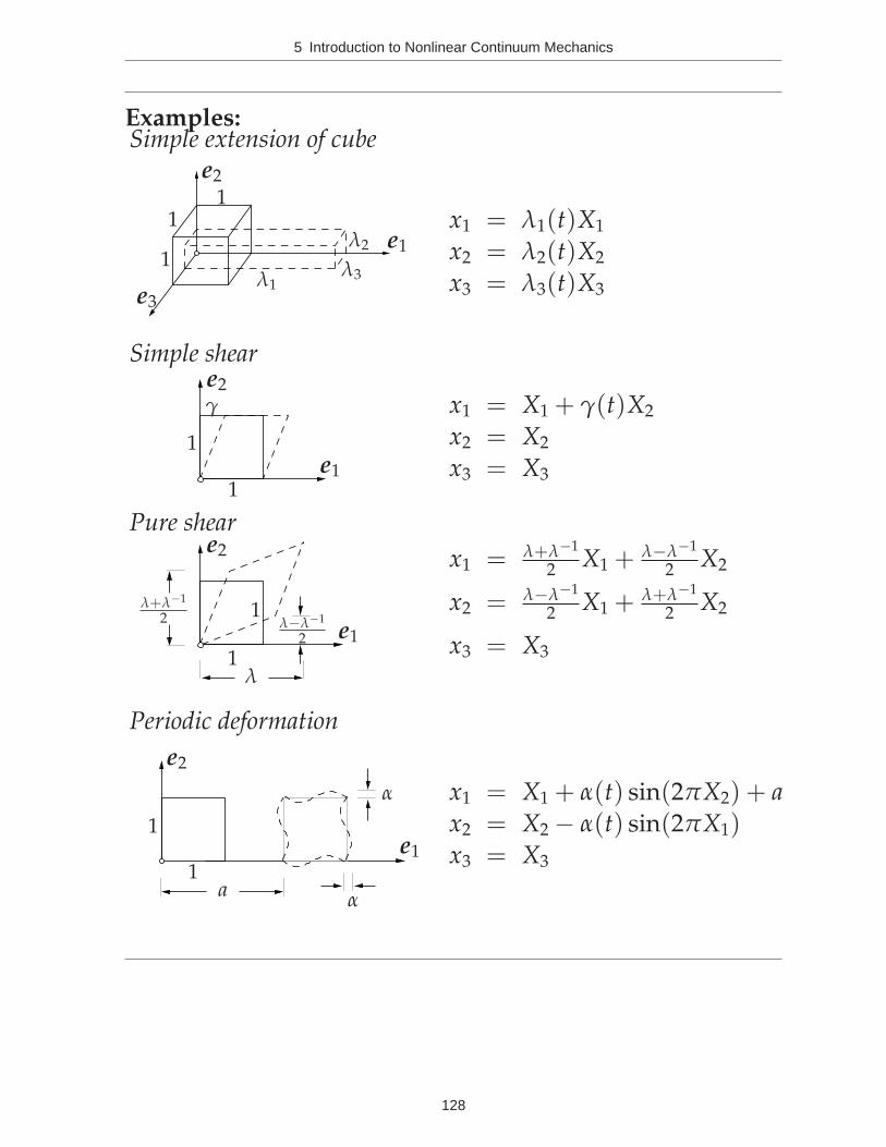
Examples:
e1
e1
e1
e1
e2
e2
e2
e2
e3
1
1
1
1
1
1
1
1
1
λ1
λ2
λ3
γ
λ+λ−1
2 λ−λ−1
2
λ
a
α
α
Simple extension of cube
Simple shear
Pure shear
Periodic deformation
x1 = λ1(t)X1
x2 = λ2(t)X2
x3 = λ3(t)X3
x1 = X1 + γ(t)X2
x2 = X2
x3 = X3
x1 = λ+λ−1
2 X1 + λ−λ−1
2 X2
x2 = λ−λ−1
2 X1 + λ+λ−1
2 X2
x3 = X3
x1 = X1 + α(t) sin(2πX2) + a
x2 = X2 − α(t) sin(2πX1)x3 = X3
128
5 Introduction to Nonlinear Continuum Mechanics
5.1.2 Velocity and Acceleration
Recall the definition of motion in (5.1.2),
x := ϕ(X, t) = ϕt(X) = ϕX(t) (5.1.5)
where ϕt(X) denotes the configuration of B at time t and
ϕX(t) is the path of the particle P.
5.1.2.1 Material Velocity and Acceleration
We can now define the material velocity
V t(X) := ∂tϕ(X, t) =d
dtϕX(t) , (5.1.6)
and the material acceleration
At(X) := ∂tV(X, t) =d
dtV X(t) (5.1.7)
of the motion. It is important to notice that both the material
velocity V(X, t) and the material acceleration A(X, t) belong
to the current configuration S but are functions of material
coordinates X and time t.
5.1.2.2 Spatial Velocity and Acceleration
The spatial counterparts of the rates of material description
of the motion can be obtained by reparameterizing the func-
tional dependency of these fields in terms of spatial coor-
dinates x. The spatial velocity and the spatial acceleration are
then defined as
v(x, t) := V(ϕ−1t (x), t) = V t(X) ϕ−1
t (x) , (5.1.8)
and
a(x, t) := A(ϕ−1t (x), t) = At(X) ϕ−1
t (x) , (5.1.9)
respectively. The path ϕX(t) is called the integral curve of v.
129
5 Introduction to Nonlinear Continuum Mechanics
5.1.2.3 Material Time Derivative of Spatial Fields
Consider a spatial field
f (x, t) : ϕt(B) ×R+ → R .
The material time derivative of f (x, t) is defined as
D
Dtf (x, t) = f (x, t) :=
∂
∂tf (x, t) + ∇x f · v (5.1.10)
For F(X, t) := f (x, t) ϕt(X), the following equality
∂
∂tF(X, t) = f (x, t) (5.1.11)
holds. An immediate example is the spatial acceleration
a(x, t) that is none other than the material time derivative of
the spatial velocity
a(x, t) := At(X) ϕ−1t (x) = ∂tv + ∇xv · v . (5.1.12)
where ∇xv stands for the spatial gradient of velocity.
130
5 Introduction to Nonlinear Continuum Mechanics
Example: Rigid Body Motion Chadwick (1976), p.52
The rigid body motion of a body is described by
x = ϕ(X, t) = c(t) + Q(t) · X ,
where Q is proper orthogonal, i.e. Q · QT = 1 and detQ =
+1. In rigid motion the distance between two points does
not change. That is, for T := XB − X A and t := xB − xA =
Q · T with xA,B = ϕ(XA,B, t), we end up with the identity
||t|| :=√
t · t =√
(Q · T) · (Q · T) =√
T · (QT · Q · T) = ||T|| .
The motion can be then inverted to obtain
X = ϕ−1t (x) = QT · (x − c) .
The material velocity and material acceleration
V t(X) := ∂tϕ(X, t) = c + Q · X
At(X) := ∂tV(X, t) = c + Q · X
The spatial velocity and spatial acceleration
v(x, t) := V(ϕ−1t (x), t) = c + Q · QT · (x − c)
a(x, t) := A(ϕ−1t (x), t) = c + Q · QT · (x − c)
Since Q · QT = 1, we have
Q · QT = −Q · QT
= −(Q · QT)T
Therefore,
Ω := Q · QT = −ΩT
131
5 Introduction to Nonlinear Continuum Mechanics
is a skew-symmetric tensor, which has an associated axial
vector ω ∈ R3 defined by
Ω · β = ω × β ∀β ∈ R3 .
Furthermore, it can be shown that
Q · QT = Ω − Q · QT
= Ω + Ω2 ,
Q ·QT · β = Ω · β + Ω2 · β = ω× β + ω× (ω× β) ∀β ∈ R3 .
Incorparating these results in the spatial velocity and spatial
acceleration expressions for β ≡ (x − c), we end up with
v(x, t) = c + ω × (x − c)
a(x, t) = c + ω × (x − c) + ω × [ω × (x − c)]
The latter can also be obtained by taking the material time
derivative of the spatial velocity field as described in (5.1.12).
a(x, t) = ∂tv + ∇xv · v
= ∂t[c + ω × (x − c)]
+ ∇x[c + ω × (x − c)] · [c + ω × (x − c)]
= c + ω × (x − c) − ω × c
+ ω × [c + ω × (x − c)]
= c + ω × (x − c) + ω × [ω × (x − c)]
132
5 Introduction to Nonlinear Continuum Mechanics
5.1.3 Fundamental Geometric Maps
This section is devoted to the geometric mapping of basic
tangential, normal and volumetric objects.
5.1.3.1 Deformation Gradient. Tangent Map
Xx
B S
ϕt(X)
F := ∇X ϕt(X)T
t
TXB Tx S
ΘR
χ0(Θ) χt(Θ)
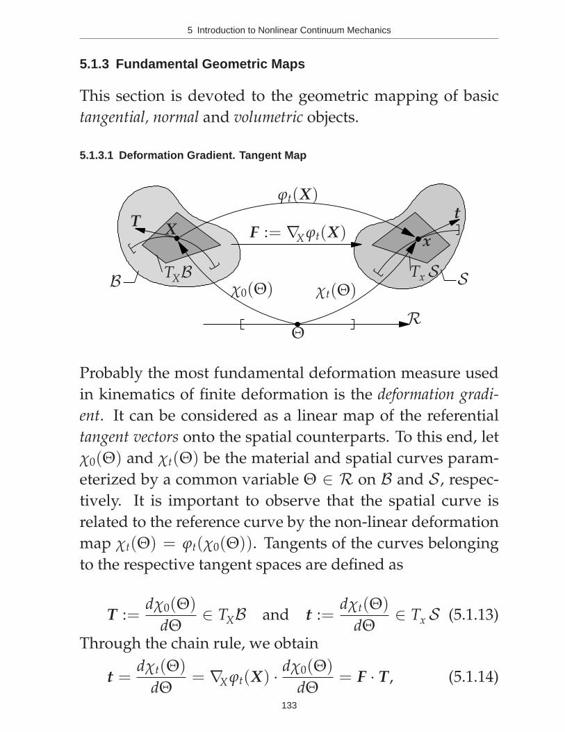
Probably the most fundamental deformation measure used
in kinematics of finite deformation is the deformation gradi-
ent. It can be considered as a linear map of the referential
tangent vectors onto the spatial counterparts. To this end, let
χ0(Θ) and χt(Θ) be the material and spatial curves param-
eterized by a common variable Θ ∈ R on B and S , respec-
tively. It is important to observe that the spatial curve is
related to the reference curve by the non-linear deformation
map χt(Θ) = ϕt(χ0(Θ)). Tangents of the curves belonging
to the respective tangent spaces are defined as
T :=dχ0(Θ)
dΘ∈ TXB and t :=
dχt(Θ)
dΘ∈ Tx S (5.1.13)
Through the chain rule, we obtain
t =dχt(Θ)
dΘ= ∇X ϕt(X) · dχ0(Θ)
dΘ= F · T , (5.1.14)
133
5 Introduction to Nonlinear Continuum Mechanics
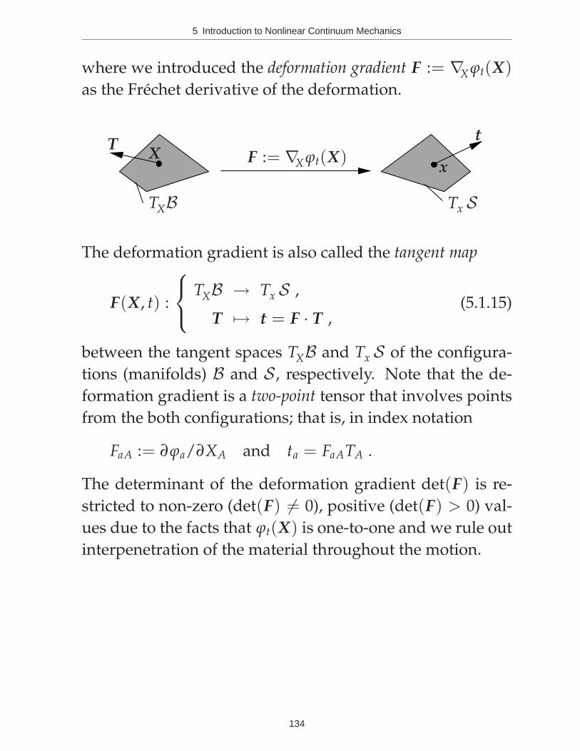
where we introduced the deformation gradient F := ∇X ϕt(X)
as the Frechet derivative of the deformation.
Xx
F := ∇X ϕt(X)T
t
TXB Tx S
The deformation gradient is also called the tangent map
F(X, t) :
TXB → Tx S ,
T 7→ t = F · T ,(5.1.15)
between the tangent spaces TXB and Tx S of the configura-
tions (manifolds) B and S , respectively. Note that the de-
formation gradient is a two-point tensor that involves points
from the both configurations; that is, in index notation
FaA := ∂ϕa/∂XA and ta = FaATA .
The determinant of the deformation gradient det(F) is re-
stricted to non-zero (det(F) 6= 0), positive (det(F) > 0) val-
ues due to the facts that ϕt(X) is one-to-one and we rule out
interpenetration of the material throughout the motion.
134
5 Introduction to Nonlinear Continuum Mechanics
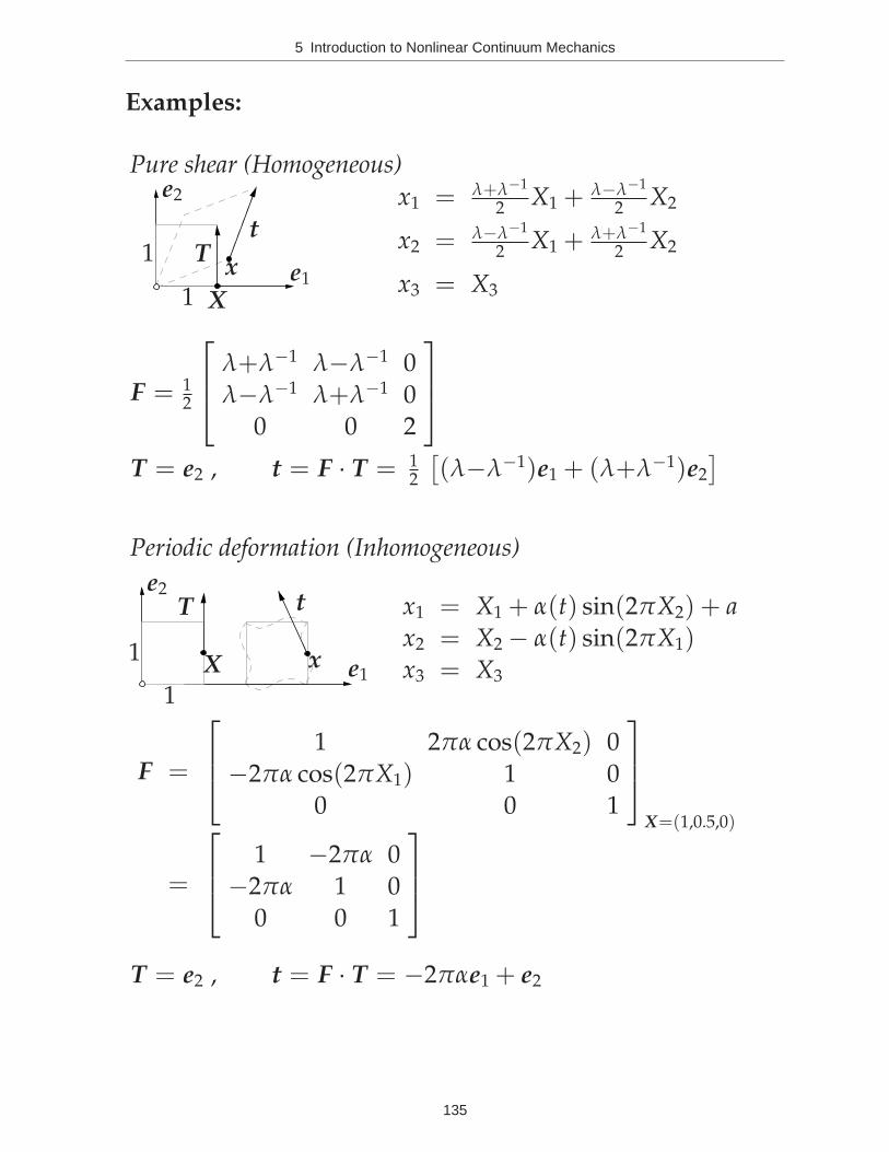
Examples:
e1
e1
e2
e2
1
1
1
1
X
X
x
x
T
Tt
t
Pure shear (Homogeneous)
Periodic deformation (Inhomogeneous)
x1 = λ+λ−1
2 X1 + λ−λ−1
2 X2
x2 = λ−λ−1
2 X1 + λ+λ−1
2 X2
x3 = X3
F = 12
λ+λ−1 λ−λ−1 0
λ−λ−1 λ+λ−1 0
0 0 2
T = e2 , t = F · T = 12
[
(λ−λ−1)e1 + (λ+λ−1)e2
]
x1 = X1 + α(t) sin(2πX2) + a
x2 = X2 − α(t) sin(2πX1)x3 = X3
F =
1 2πα cos(2πX2) 0
−2πα cos(2πX1) 1 0
0 0 1
X=(1,0.5,0)
=
1 −2πα 0
−2πα 1 0
0 0 1
T = e2 , t = F · T = −2παe1 + e2
135
5 Introduction to Nonlinear Continuum Mechanics
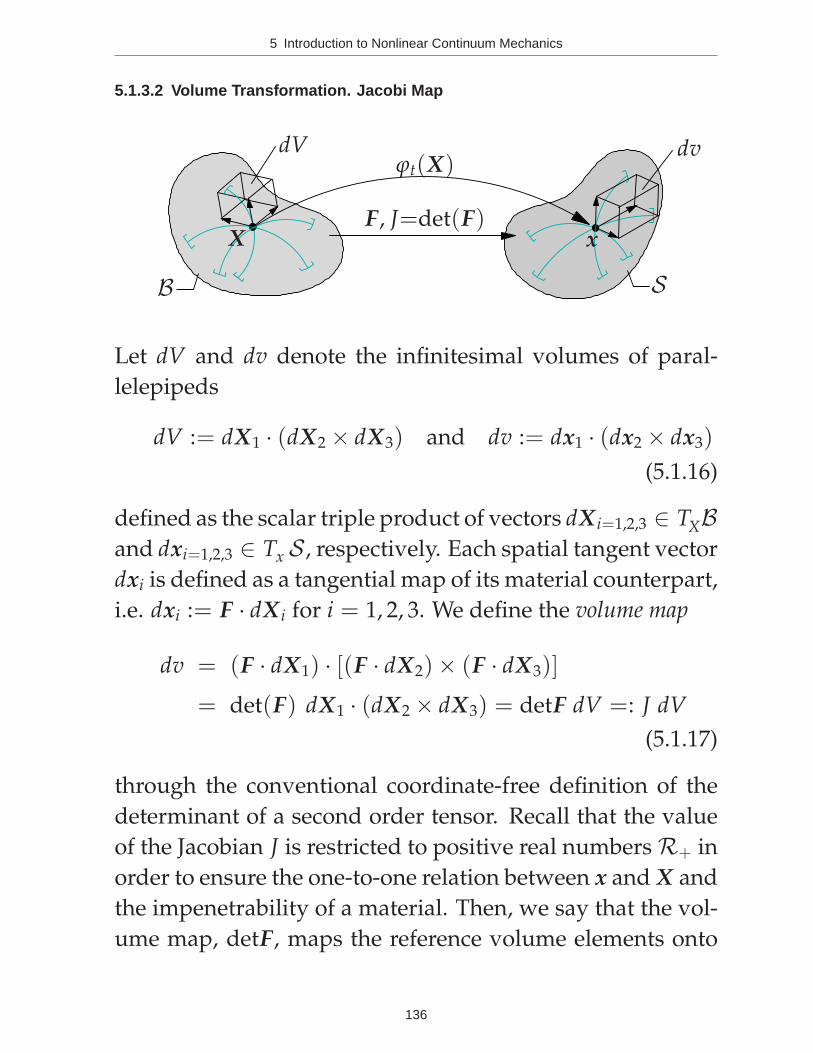
5.1.3.2 Volume Transformation. Jacobi Map
X x
B S
ϕt(X)
F, J=det(F)
dV dv
Let dV and dv denote the infinitesimal volumes of paral-
lelepipeds
dV := dX1 · (dX2 × dX3) and dv := dx1 · (dx2 × dx3)
(5.1.16)
defined as the scalar triple product of vectors dX i=1,2,3 ∈ TXBand dxi=1,2,3 ∈ Tx S , respectively. Each spatial tangent vector
dxi is defined as a tangential map of its material counterpart,
i.e. dxi := F · dX i for i = 1, 2, 3. We define the volume map
dv = (F · dX1) · [(F · dX2) × (F · dX3)]
= det(F) dX1 · (dX2 × dX3) = detF dV =: J dV
(5.1.17)
through the conventional coordinate-free definition of the
determinant of a second order tensor. Recall that the value
of the Jacobian J is restricted to positive real numbers R+ in
order to ensure the one-to-one relation between x and X and
the impenetrability of a material. Then, we say that the vol-
ume map, detF, maps the reference volume elements onto
136
5 Introduction to Nonlinear Continuum Mechanics
their spatial counterparts
J = detF :=
R+ → R+ ,
dV 7→ dv = detFdV .(5.1.18)
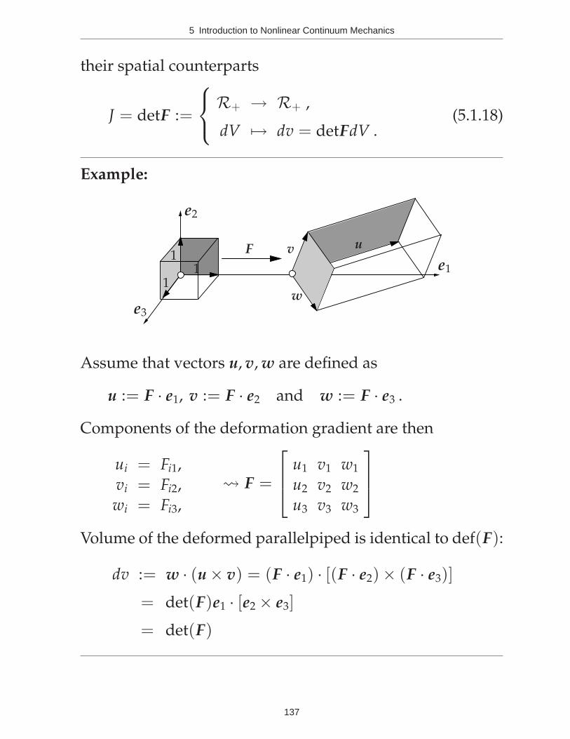
Example:
e1
e2
e3
11
1
F uv
w
Assume that vectors u, v, w are defined as
u := F · e1, v := F · e2 and w := F · e3 .
Components of the deformation gradient are then
ui = Fi1,
vi = Fi2,
wi = Fi3,
F =
u1 v1 w1
u2 v2 w2
u3 v3 w3
Volume of the deformed parallelpiped is identical to def(F):
dv := w · (u × v) = (F · e1) · [(F · e2) × (F · e3)]
= det(F)e1 · [e2 × e3]
= det(F)
137
5 Introduction to Nonlinear Continuum Mechanics
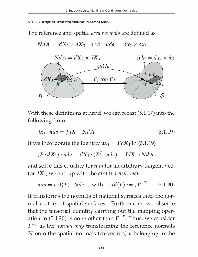
5.1.3.3 Adjoint Transformation. Normal Map
The reference and spatial area normals are defined as
NdA := dX2 × dX3 and nda := dx2 × dx3 .
X x
B S
ϕt(X)
F, cof(F)
NdA = dX2 × dX3 nda = dx2 × dx3
dX2dX3dx2
dx3
With these definitions at hand, we can recast (5.1.17) into the
following from
dx1 · nda = JdX1 · NdA . (5.1.19)
If we incorporate the identity dx1 = FdX1 in (5.1.19)
(F · dX1) · nda = dX1 · (FT · nda) = JdX1 · NdA ,
and solve this equality for nda for an arbitrary tangent vec-
tor dX1, we end up with the area (normal) map
nda = cof(F) · NdA with cof(F) := JF−T . (5.1.20)
It transforms the normals of material surfaces onto the nor-
mal vectors of spatial surfaces. Furthermore, we observe
that the tensorial quantity carrying out the mapping oper-
ation in (5.1.20) is none other than F−T. Thus, we consider
F−T as the normal map transforming the reference normals
N onto the spatial normals (co-vectors) n belonging to the
138
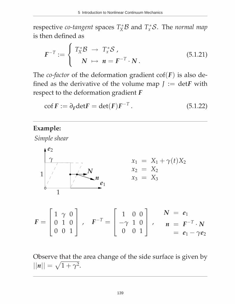
5 Introduction to Nonlinear Continuum Mechanics
respective co-tangent spaces T ∗XB and T ∗
x S . The normal map
is then defined as
F−T :=
T ∗XB → T ∗
x S ,
N 7→ n = F−T · N .(5.1.21)
The co-factor of the deformation gradient cof(F) is also de-
fined as the derivative of the volume map J := detF with
respect to the deformation gradient F
cof F := ∂FdetF = det(F)F−T . (5.1.22)
Example:
e1
e2
1
1
γ
Nn
Simple shear
x1 = X1 + γ(t)X2
x2 = X2
x3 = X3
F =
1 γ 0
0 1 0
0 0 1
, F−T =
1 0 0
−γ 1 0
0 0 1
,
N = e1
n = F−T · N
= e1 − γe2
Observe that the area change of the side surface is given by
||n|| =√
1 + γ2.
139
5 Introduction to Nonlinear Continuum Mechanics
5.1.4 Deformation and Strain Tensors
This section outlines the fundamental deformation and strain
tensors that often enter the strain energy functions.
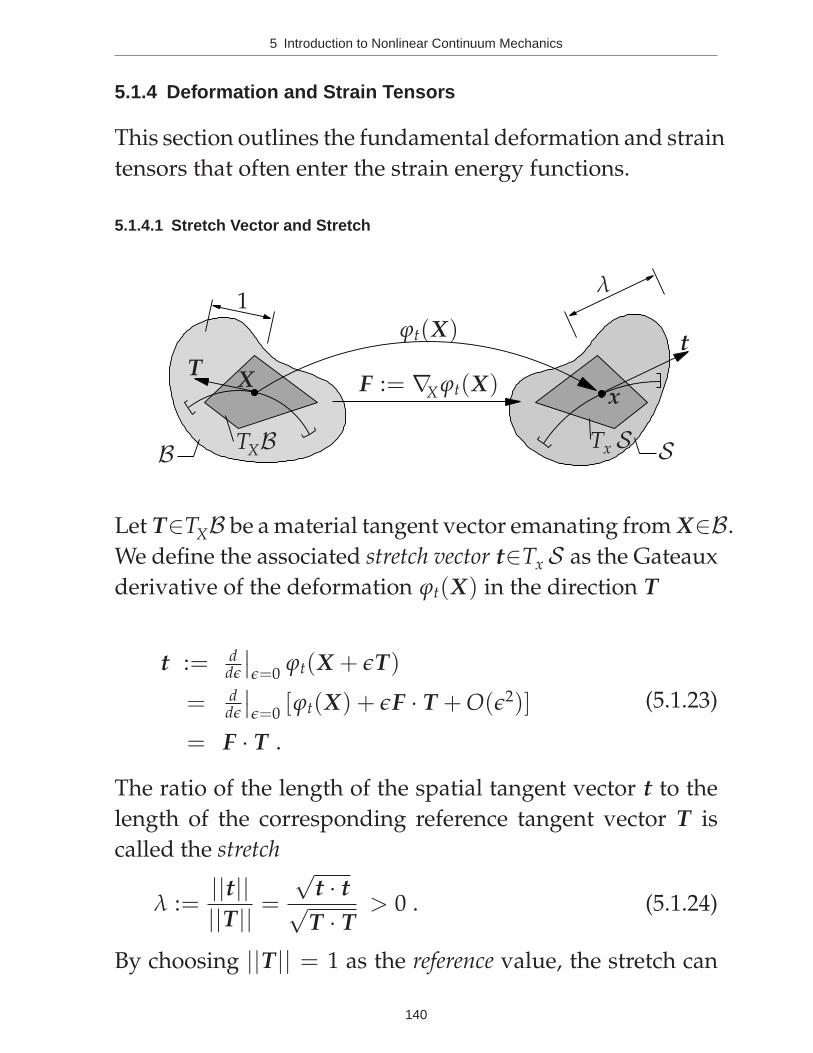
5.1.4.1 Stretch Vector and Stretch
Xx
B S
ϕt(X)
F := ∇X ϕt(X)T
t
TXB Tx S
1λ
Let T∈TXB be a material tangent vector emanating from X∈B.
We define the associated stretch vector t∈Tx S as the Gateaux
derivative of the deformation ϕt(X) in the direction T
t := ddǫ
∣
∣
ǫ=0ϕt(X + ǫT)
= ddǫ
∣
∣
ǫ=0[ϕt(X) + ǫF · T + O(ǫ2)]
= F · T .
(5.1.23)
The ratio of the length of the spatial tangent vector t to the
length of the corresponding reference tangent vector T is
called the stretch
λ :=||t||||T|| =
√t · t√
T · T> 0 . (5.1.24)
By choosing ||T|| = 1 as the reference value, the stretch can
140
5 Introduction to Nonlinear Continuum Mechanics
be expressed as
λ =√
t · t =√
(F · T) · (F · T)
=√
T · (FT · F) · T =√
T · C · T =: ||T||C ,(5.1.25)
where we already introduced the right Cauchy-Green tensor
C := FT · F , CAB = FaAFaB . (5.1.26)
It is important to observe that the right Cauchy-Green tensor
is symmetric and positive-definite; that is,
C = CT = (FT · F)T = FT · F and T ·C ·T ≥ 0 ∀T ∈ R3 .
(5.1.27)
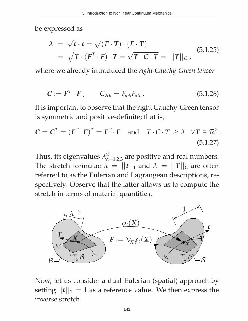
Thus, its eigenvalues λ2α=1,2,3 are positive and real numbers.
The stretch formulae λ = ||t||1 and λ = ||T||C are often
referred to as the Eulerian and Lagrangean descriptions, re-
spectively. Observe that the latter allows us to compute the
stretch in terms of material quantities.
Xx
B S
ϕt(X)
F := ∇X ϕt(X)T
t
TXB Tx S
λ−1 1
Now, let us consider a dual Eulerian (spatial) approach by
setting ||t||1 = 1 as a reference value. We then express the
inverse stretch
141
5 Introduction to Nonlinear Continuum Mechanics
λ−1 =√
T · T =√
(F−1 · t) · (F−1 · t)
=√
t · (F−T · F−1) · t =√
t · b−1t =: ||t||b−1
(5.1.28)
in terms of the inverse left Cauchy-Green tensor b−1
b−1 := F−T · F−1 , b−1ab = F−1
Aa F−1Ab . (5.1.29)
The left Cauchy-Green tensor b is then defined as
b := F · FT , bab = FaAFbA . (5.1.30)
From this definition, we readily note that the left Cauchy-
Green (Finger) tensor is also symmetric and positive-definite,
i.e.
b = bT = (F · FT)T = F · FT and t · b · t ≥ 0 ∀t ∈ R3 .
(5.1.31)
In (5.1.25) and (5.1.28), we observe that C and b−1 act as met-
ric tensors in the respective Lagrangean and Eulerian de-
scription of the length deformation.
5.1.4.2 Strain Tensors
Having the stretch defined in (5.1.25), we are now in a posi-
tion to define the Green-Lagrange strain tensor. The Green-
Lagrange strain measure εGL, Lagrangean strain measure,
compares the squared lengths of the spatial vector ||t||21 =
||T||2C and the reference vector ||T ||21 = 1 in an additive man-
ner
εGL := 12 [λ2 − 1] . (5.1.32)
142
5 Introduction to Nonlinear Continuum Mechanics
Insertion of the above definitions yields
εGL := 12 [||T||2C − ||T||21]
= 12 [T · C · T − T · 1 · T ]
= T · 12 [C − 1] · T =: T · E · T .
(5.1.33)
The Green-Lagrange strain tensor E is then defined as
E := 12 [C − 1] , EAB = 1
2 [CAB − δAB] . (5.1.34)
Analogous to the dual approach we considered for the in-
verse stretch, the Eulerian strain measure, the so-called Al-
mansi strain measure is defined as
εA := 12 [1 − λ−2] , (5.1.35)
where ||t||21 = 1 and ||t||2b−1 = λ−2. Incoporating these defi-
nitions, we have
εA := 12 [||t||21 − ||t||2
b−1]
= 12 [t · 1 · t − t · b−1 · t]
= t · 12 [1 − b−1] · t =: t · e · t .
(5.1.36)
with
e := 12 [1 − b−1] , eab = 1
2 [δab − b−1ab ] . (5.1.37)
denoting the Eulerian Almansi strain tensor.
It is important to note that linearization of the both strain
tensors, E and e about the undeformed state leads to the
strain tensor ε=sym(∇xu) in the geometrically linear theory.
ε = sym(∇xu) = Lin|F=1E = Lin|F=1e (5.1.38)
143
5 Introduction to Nonlinear Continuum Mechanics
5.1.5 Material and Spatial Velocity Gradients
Recall that the stretch vector t = F · T ∈ Tx S was defined
as a tangent map of the material tangent T ∈ TXB. The total
time derivative of t is then given by
t = F · T =: L · T , (5.1.39)
where the time derivative of the deformation gradient can
be expressed as
L := F =∂
∂t(∇X ϕ(X, t)) = ∇X
(
∂
∂tϕ(X, t)
)
= ∇XV(X, t)
(5.1.40)
the gradient of the material velocity with respect to the ma-
terial coordinates. Therefore, we call L the material velocity
gradient that maps the material tangent vector T on the to-
tal time derivative of its spatial counter part as shown in
(5.1.39).
The material vector T in (5.1.39) can be expressed as T =
F−1 · t. Here, the inverse of the deformation gradient can be
obtained thorugh F−1 = ∇xX. Then, the rate of the stretch
vector assumes the form
t = (F · F−1) · t =: l · t (5.1.41)
where we introduced the spatial velocity gradient
l := L · F−1 = ∇XV(X, t) · ∇xX = ∇xv(x, t) (5.1.42)
by using the relation v(x, t) = V(X, t) ϕ−1t (X).
144
5 Introduction to Nonlinear Continuum Mechanics
Xx
F
L
l
T
t
t
TXB Tx S
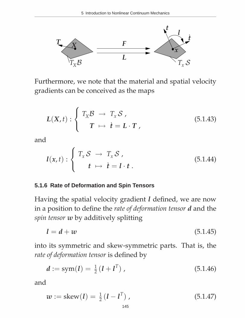
Furthermore, we note that the material and spatial velocity
gradients can be conceived as the maps
L(X, t) :
TXB → Tx S ,
T 7→ t = L · T ,(5.1.43)
and
l(x, t) :
Tx S → Tx S ,
t 7→ t = l · t .(5.1.44)
5.1.6 Rate of Deformation and Spin Tensors
Having the spatial velocity gradient l defined, we are now
in a position to define the rate of deformation tensor d and the
spin tensor w by additively splitting
l = d + w (5.1.45)
into its symmetric and skew-symmetric parts. That is, the
rate of deformation tensor is defined by
d := sym(l) = 12 (l + lT) , (5.1.46)
and
w := skew(l) = 12 (l − lT) , (5.1.47)
145
5 Introduction to Nonlinear Continuum Mechanics
denotes the spin tensor. Therefore the map (5.1.41) can also
be additively decomposed into
t = l · t = d · t + w · t , (5.1.48)
in which the part d · t related with the rate of stretching and
the part w · t associated with rotation.
In order to interpret the geometrical meaning of the rate of
deformation tensor, we consider the time rate of square of
the stretch by following its material description in (5.1.25)
d
dt(λ2) = 2λλ = T · C · T . (5.1.49)
Since C = FT · F and t = F · T , we have C = FT · F + FT · F
and T = F−1 · t. Insertion of these results leads us to
2λλ = T · C · T
= (F−1 · t) · (FT · F + FT · F) · (F−1 · t)
= t · (F−T · FT+ F · F−1) · t
= t · (lT + l) · t = t · 2d · t
(5.1.50)
Introducing a unit vector g, i.e. ||g||=1, parallel to t = λg,
we end up with the time derivative of the logarithmic strain
εln := ln(λ) in the direction g
εln = ˙ln λ = λ/λ = d : (g ⊗ g) = g · d · g
identical to the component dgg = g · d · g of the rate of de-
formation tensor. This means, if we had g = nα with nα de-
146
5 Introduction to Nonlinear Continuum Mechanics
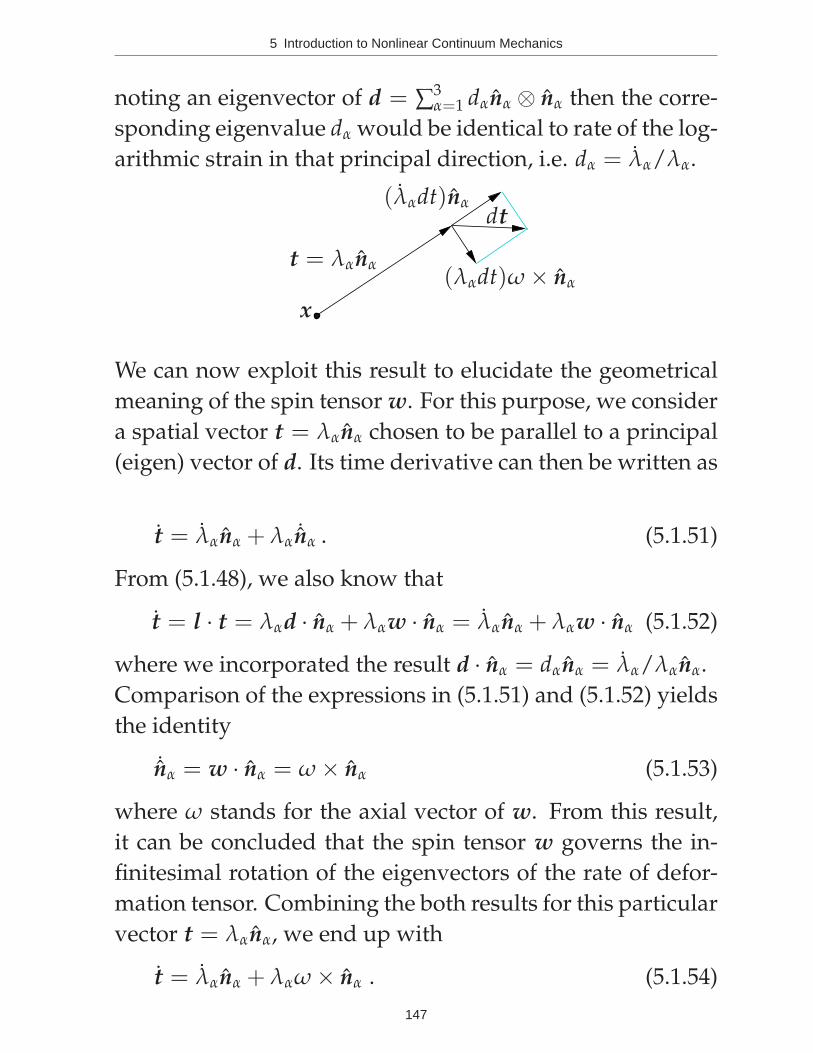
noting an eigenvector of d = ∑3α=1 dαnα ⊗ nα then the corre-
sponding eigenvalue dα would be identical to rate of the log-
arithmic strain in that principal direction, i.e. dα = λα/λα.
x
t = λαnα
dt(λαdt)nα
(λαdt)ω × nα
We can now exploit this result to elucidate the geometrical
meaning of the spin tensor w. For this purpose, we consider
a spatial vector t = λαnα chosen to be parallel to a principal
(eigen) vector of d. Its time derivative can then be written as
t = λαnα + λα˙nα . (5.1.51)
From (5.1.48), we also know that
t = l · t = λαd · nα + λαw · nα = λαnα + λαw · nα (5.1.52)
where we incorporated the result d · nα = dαnα = λα/λαnα.
Comparison of the expressions in (5.1.51) and (5.1.52) yields
the identity
˙nα = w · nα = ω × nα (5.1.53)
where ω stands for the axial vector of w. From this result,
it can be concluded that the spin tensor w governs the in-
finitesimal rotation of the eigenvectors of the rate of defor-
mation tensor. Combining the both results for this particular
vector t = λαnα, we end up with
t = λαnα + λαω × nα . (5.1.54)
147
5 Introduction to Nonlinear Continuum Mechanics
5.1.7 Push-Forward and Pull-Back Relations
Lagrangean and Eulerian fields are related through the push-
forward and pull-back operations. For the rate of deformation
tensors, for example, we observe in (5.1.50) that
d = F−T · 12 C · F−1 (5.1.55)
holds. We then say that the rate of deformation tensor d is
the push-forward of the time derivative of the Green-Lagrange
strain tensor E ≡ 12 C and denote the push-forward opera-
tion
d = ϕ∗(E) = ϕ∗(12 C) := F−T ·
(
12 C
)
· F−1 , (5.1.56)
or in indicial notation
dab = F−1Aa
12 CABF−1
Bb .
Analogously, we have the identity
12 C = E = FT · d · F (5.1.57)
where 12 C = E is the pull-back of the rate of deformation
tensor d
E = 12 C = ϕ∗(d) = FT · d · F , (5.1.58)
or in indicial notation
EAB = 12 CAB = FaAdabFbB .
The Almansi strain tensor and the Green-Lagrange strain
tensor are also related through the pull-back and push-forward
maps, i.e. E = FT · e · F. The Almansi strain tensor e is the
push-forward of the Green-Lagrange strain tensor E
e = ϕ∗(E) := F−T · E · F−1 , eab = F−1Aa EABF−1
Bb . (5.1.59)
148
5 Introduction to Nonlinear Continuum Mechanics
Analogously, E is the pull-back of the Almansi strain tensor e
E = ϕ∗(e) = FT · e · F , EAB = FaAeabFbB . (5.1.60)
Similar pull-back and push-forward relations exist also among
the different stress measures that will be discussed in the
next chapter.
5.1.8 Lie Derivative of Spatial Fields
The Lie derivative of a spatial field, say f (x, t), is defined as
£v f (x, t) := ϕ∗
d
dt[ϕ∗( f (x, t))]
, (5.1.61)
which is none other than the push-forward of the time deriva-
tive of the pull-back of the spatial field f (x, t).
For instance, it can be readily shown that the rate of defor-
mation tensor d is the Lie derivative of the Almansi strain
tensor e. Since we have shown that the rate of deformation
tensor d is push-forward of E, d = ϕ∗(E) and the Green-
Lagrange strain tensor is pull-back of the Almansi strain ten-
sor E = ϕ∗(e), we have
£ve := ϕ∗
d
dt[ϕ∗(e)]
= ϕ∗
d
dt[E]
= ϕ∗(E) = d .
(5.1.62)
The Lie (Oldroyd) derivatives constitute the basic class of
objective time derivatives of Eulerian objects.
149