Lecture 9 - KTH · The VC dimension The Vapnik-Chervonenkis dimension This is a measure of the...
52
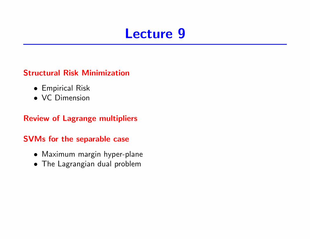
Lecture 9 Structural Risk Minimization • Empirical Risk • VC Dimension Review of Lagrange multipliers SVMs for the separable case • Maximum margin hyper-plane • The Lagrangian dual problem
Transcript of Lecture 9 - KTH · The VC dimension The Vapnik-Chervonenkis dimension This is a measure of the...
Lecture 9
Structural Risk Minimization
• Empirical Risk• VC Dimension
Review of Lagrange multipliers
SVMs for the separable case
• Maximum margin hyper-plane• The Lagrangian dual problem
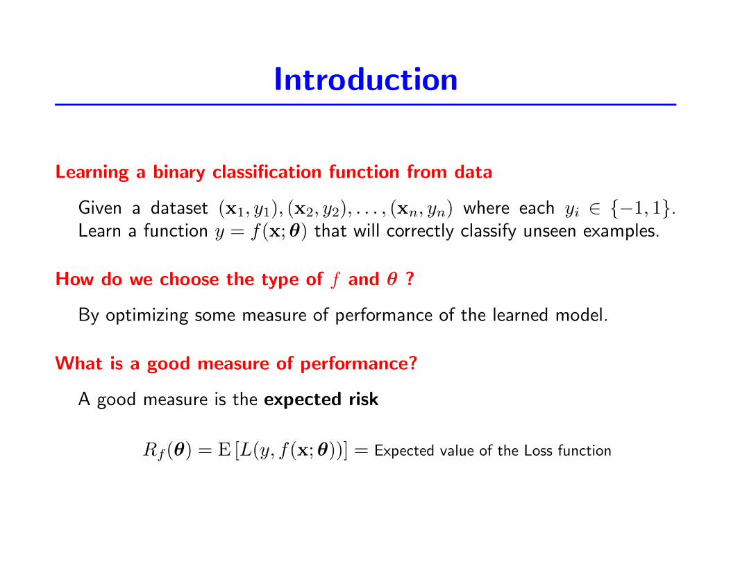
Introduction
Learning a binary classification function from data
Given a dataset (x1, y1), (x2, y2), . . . , (xn, yn) where each yi ∈ {−1, 1}.Learn a function y = f(x;θ) that will correctly classify unseen examples.
How do we choose the type of f and θ ?
By optimizing some measure of performance of the learned model.
What is a good measure of performance?
A good measure is the expected risk
Rf(θ) = E [L(y, f(x;θ))] = Expected value of the Loss function
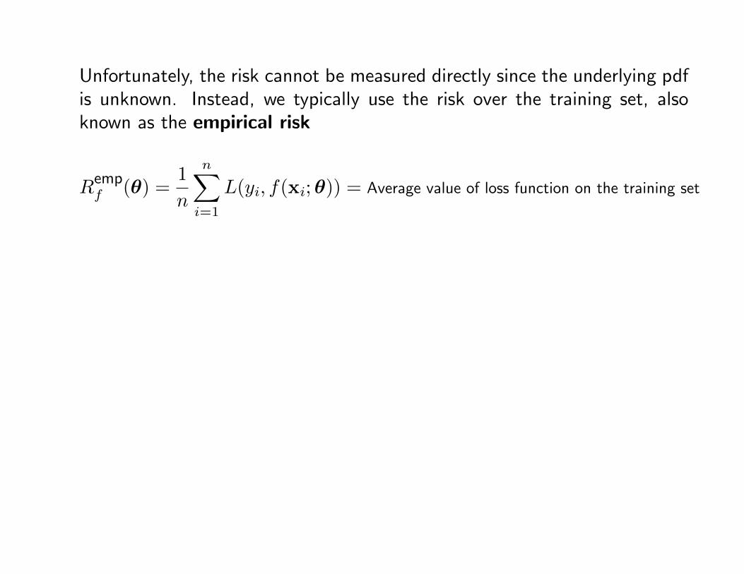
Unfortunately, the risk cannot be measured directly since the underlying pdfis unknown. Instead, we typically use the risk over the training set, alsoknown as the empirical risk
Rempf (θ) =
1
n
n∑i=1
L(yi, f(xi;θ)) = Average value of loss function on the training set
Introduction
Empirical Risk Minimization
• A formal term for a simple concept: find the function f(x) that minimizesthe average risk on the training set.
• Minimizing the empirical risk is not a bad thing to do, provided thatsufficient training data is available, since the law of large numbers ensuresthat the empirical risk will asymptotically converge to the expected risk forn→∞.
• However, for small samples, one cannot guarantee that ERM will alsominimize the expected risk. This is the all too familiar issue of generalization.
Introduction
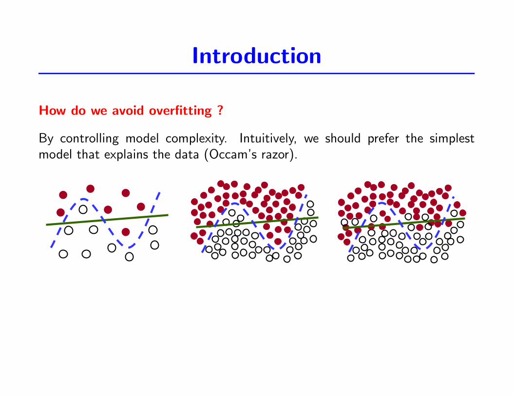
How do we avoid overfitting ?
By controlling model complexity. Intuitively, we should prefer the simplestmodel that explains the data (Occam’s razor).
Introduction to Pattern AnalysisRicardo Gutierrez-OsunaTexas A&M University
3
Introduction (2)! Empirical Risk Minimization
" A formal term for a simple concept: find the function f(x) that minimizes the average risk on the training set
" Minimizing the empirical risk is not a bad thing to do, provided that sufficient training data is available, since the law of large numbers ensures that the empirical risk will asymptotically converge to the expected risk for n!"
" However, for small samples, one cannot guarantee that ERM will also minimize the expected risk. This is the all too familiar issue of generalization
! How do we avoid overfitting? " By controlling model complexity. Intuitively, we should prefer the simplest model
that explains the data (Occam’s razor)
From [Müller et al., 2001]
The VC dimension
The Vapnik-Chervonenkis dimension
This is a measure of the complexity / capacity of a class of functions F . Itmeasures the largest number of examples that can be explained by the familyF .
Trade-off between High Capacity and Good generalization
More capacity If the family F has sufficient capacity to explain every possibledata-set =⇒ there is a risk of overfitting.
Less capacity Functions f ∈ F having small capacity may not be able toexplain our particular dataset, however, are much less likely to overfit.
How does VC-dimension characterize this trade-off?
Vapnik-Chervonenkis dimension
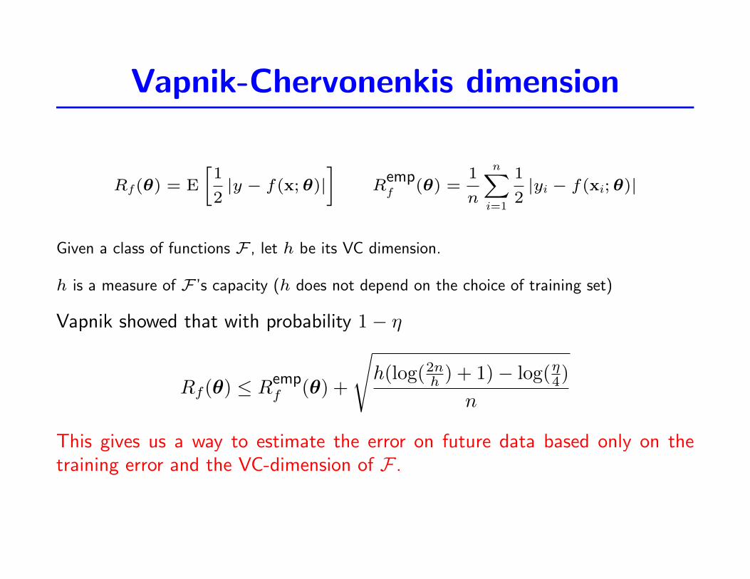
Rf(θ) = E
[1
2|y − f(x; θ)|
]R
empf (θ) =
1
n
n∑i=1
1
2|yi − f(xi; θ)|
Given a class of functions F , let h be its VC dimension.
h is a measure of F ’s capacity (h does not depend on the choice of training set)
Vapnik showed that with probability 1− η
Rf(θ) ≤ Rempf (θ) +
√h(log(2nh ) + 1)− log(η4)
n
This gives us a way to estimate the error on future data based only on thetraining error and the VC-dimension of F .
Vapnik-Chervonenkis dimension
Given F how do we define and compute h, its VC dimension?
Will now introduce the concept of shattering....
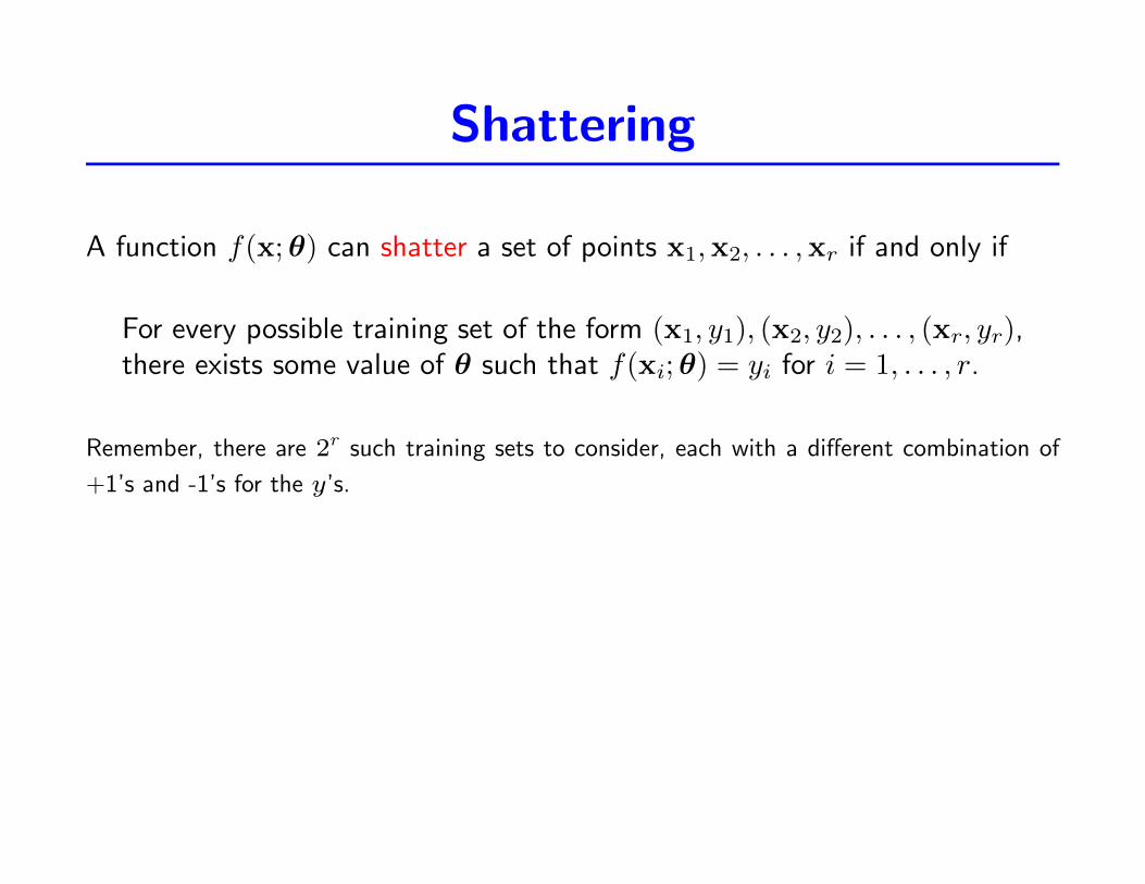
Shattering
A function f(x;θ) can shatter a set of points x1,x2, . . . ,xr if and only if
For every possible training set of the form (x1, y1), (x2, y2), . . . , (xr, yr),there exists some value of θ such that f(xi;θ) = yi for i = 1, . . . , r.
Remember, there are 2r such training sets to consider, each with a different combination of
+1’s and -1’s for the y’s.
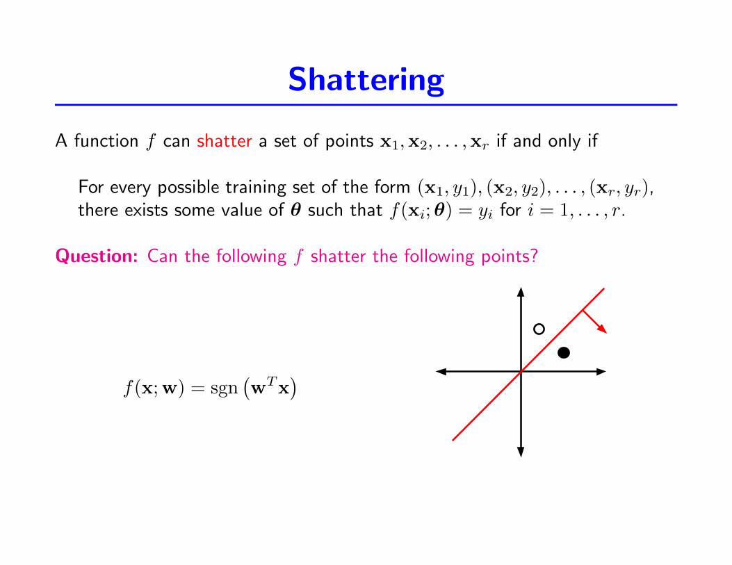
Shattering
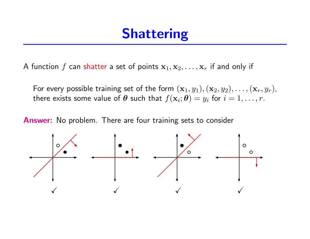
A function f can shatter a set of points x1,x2, . . . ,xr if and only if
For every possible training set of the form (x1, y1), (x2, y2), . . . , (xr, yr),there exists some value of θ such that f(xi;θ) = yi for i = 1, . . . , r.
Question: Can the following f shatter the following points?
f(x;w) = sgn(wTx
)
Shattering
A function f can shatter a set of points x1,x2, . . . ,xr if and only if
For every possible training set of the form (x1, y1), (x2, y2), . . . , (xr, yr),there exists some value of θ such that f(xi;θ) = yi for i = 1, . . . , r.
Answer: No problem. There are four training sets to consider
X X X X
Shattering
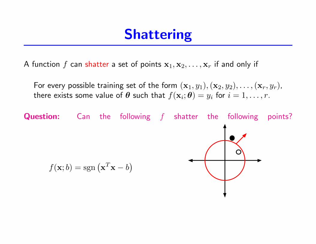
A function f can shatter a set of points x1,x2, . . . ,xr if and only if
For every possible training set of the form (x1, y1), (x2, y2), . . . , (xr, yr),there exists some value of θ such that f(xi;θ) = yi for i = 1, . . . , r.
Question: Can the following f shatter the following points?
f(x; b) = sgn(xTx− b
)
Shattering
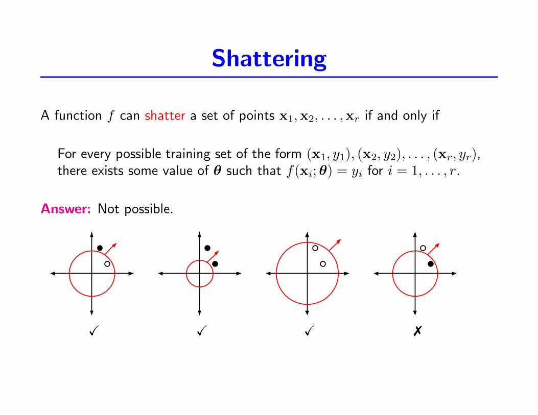
A function f can shatter a set of points x1,x2, . . . ,xr if and only if
For every possible training set of the form (x1, y1), (x2, y2), . . . , (xr, yr),there exists some value of θ such that f(xi;θ) = yi for i = 1, . . . , r.
Answer: Not possible.
X X X 7
Definition of VC dimension
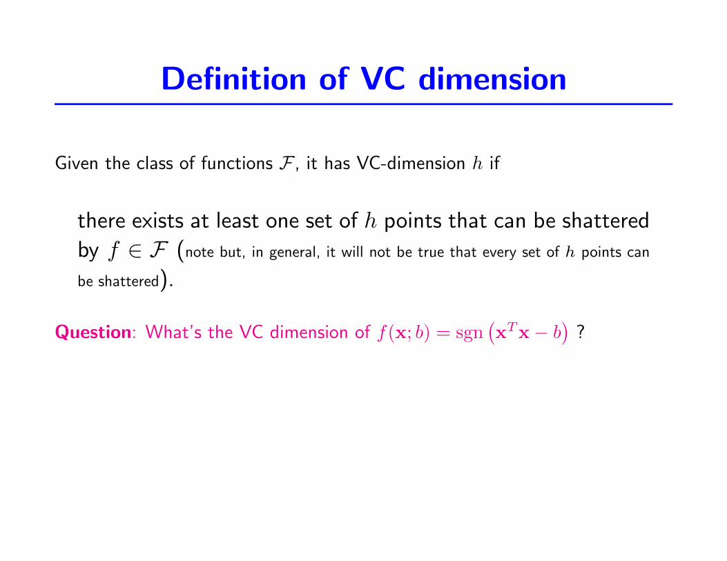
Given the class of functions F , it has VC-dimension h if
there exists at least one set of h points that can be shattered
by f ∈ F (note but, in general, it will not be true that every set of h points can
be shattered).
Question: What’s the VC dimension of f(x; b) = sgn(xTx− b
)?
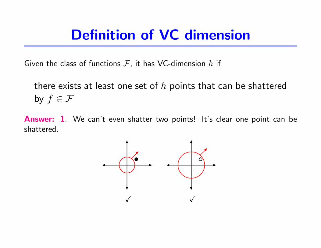
Definition of VC dimension
Given the class of functions F , it has VC-dimension h if
there exists at least one set of h points that can be shattered
by f ∈ F
Answer: 1. We can’t even shatter two points! It’s clear one point can beshattered.
X X
Definition of VC dimension
Given the class of functions F , it has VC-dimension h if
there exists at least one set of h points that can be shattered
by f ∈ F
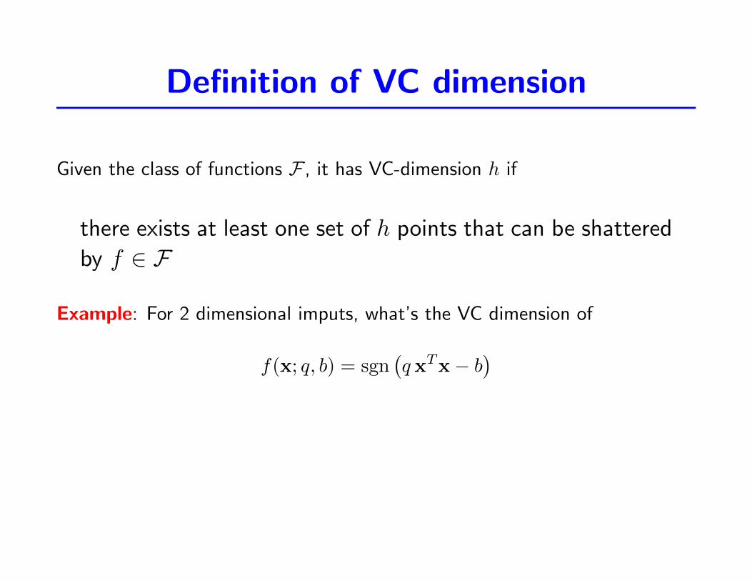
Example: For 2 dimensional imputs, what’s the VC dimension of
f(x; q, b) = sgn(q xTx− b
)
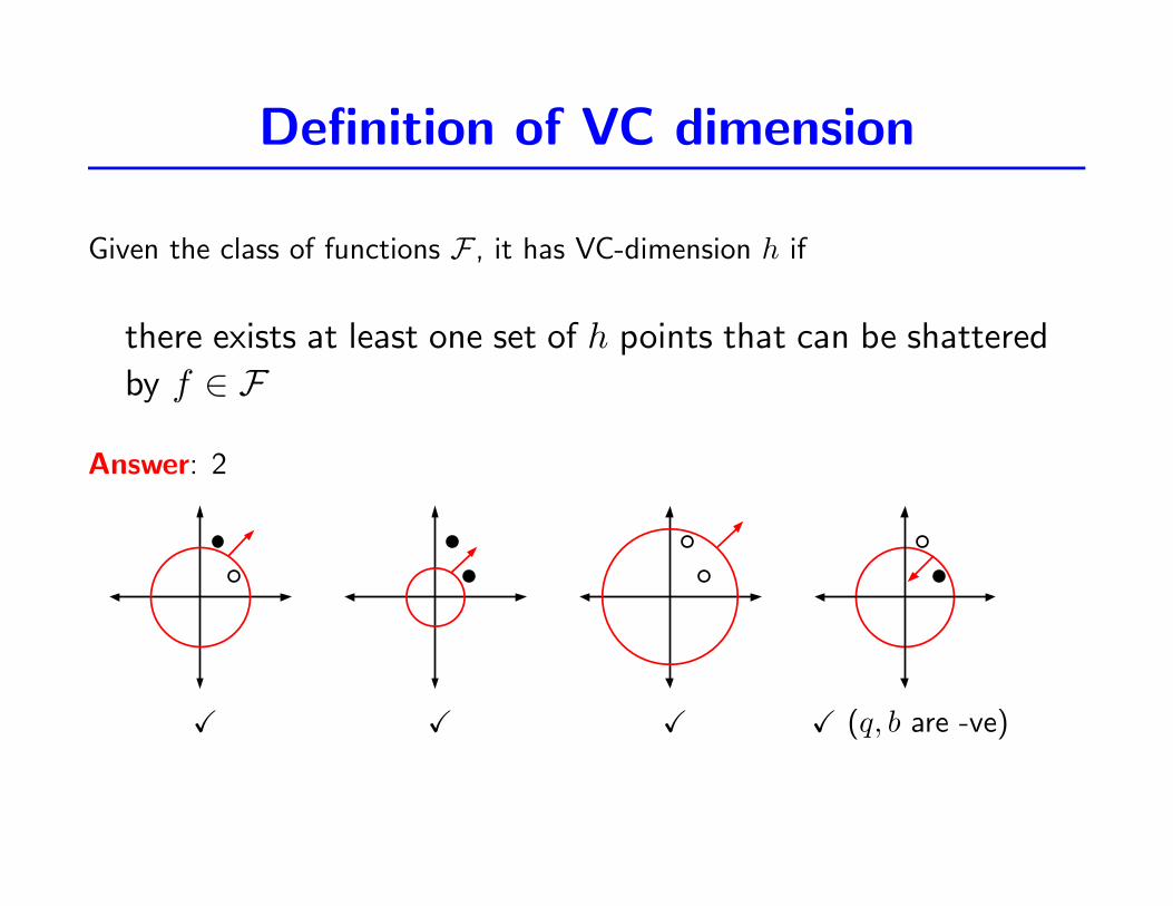
Definition of VC dimension
Given the class of functions F , it has VC-dimension h if
there exists at least one set of h points that can be shattered
by f ∈ F
Answer: 2
X X X X (q, b are -ve)
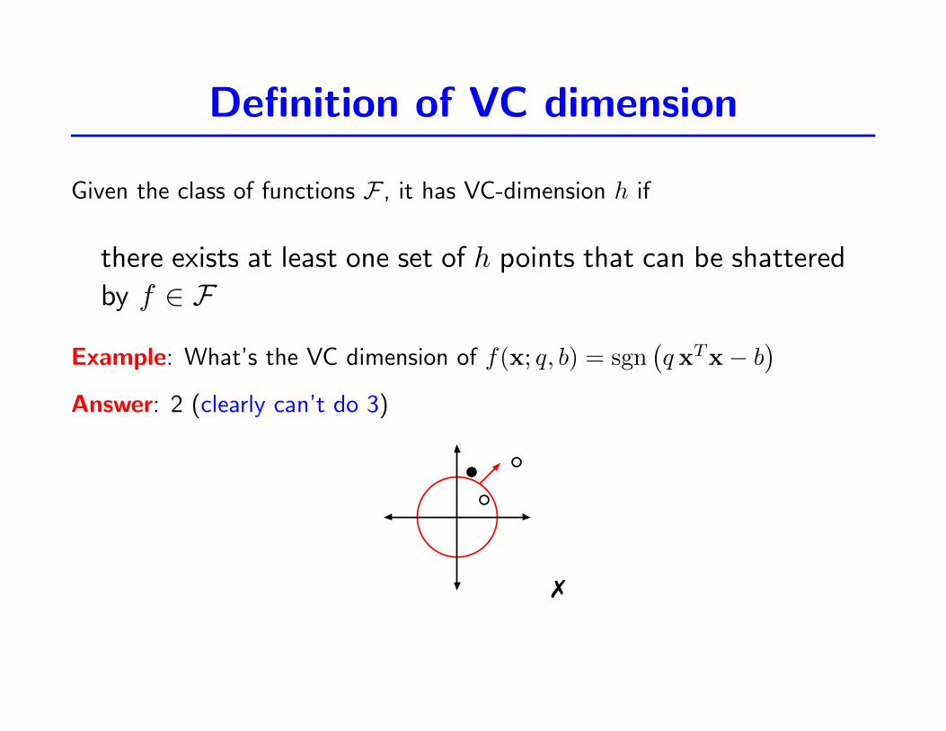
Definition of VC dimension
Given the class of functions F , it has VC-dimension h if
there exists at least one set of h points that can be shattered
by f ∈ F
Example: What’s the VC dimension of f(x; q, b) = sgn(q xTx− b
)Answer: 2 (clearly can’t do 3)
7
VC dimension of separating line
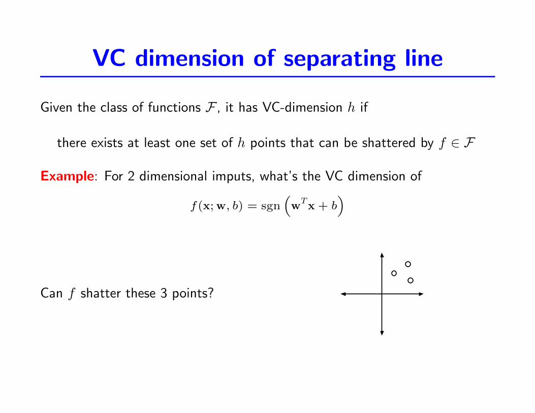
Given the class of functions F , it has VC-dimension h if
there exists at least one set of h points that can be shattered by f ∈ F
Example: For 2 dimensional imputs, what’s the VC dimension of
f(x;w, b) = sgn(wTx + b
)
Can f shatter these 3 points?
VC dimension of separating line
Given the class of functions F , it has VC-dimension h if
there exists at least one set of h points that can be shattered
by f ∈ F
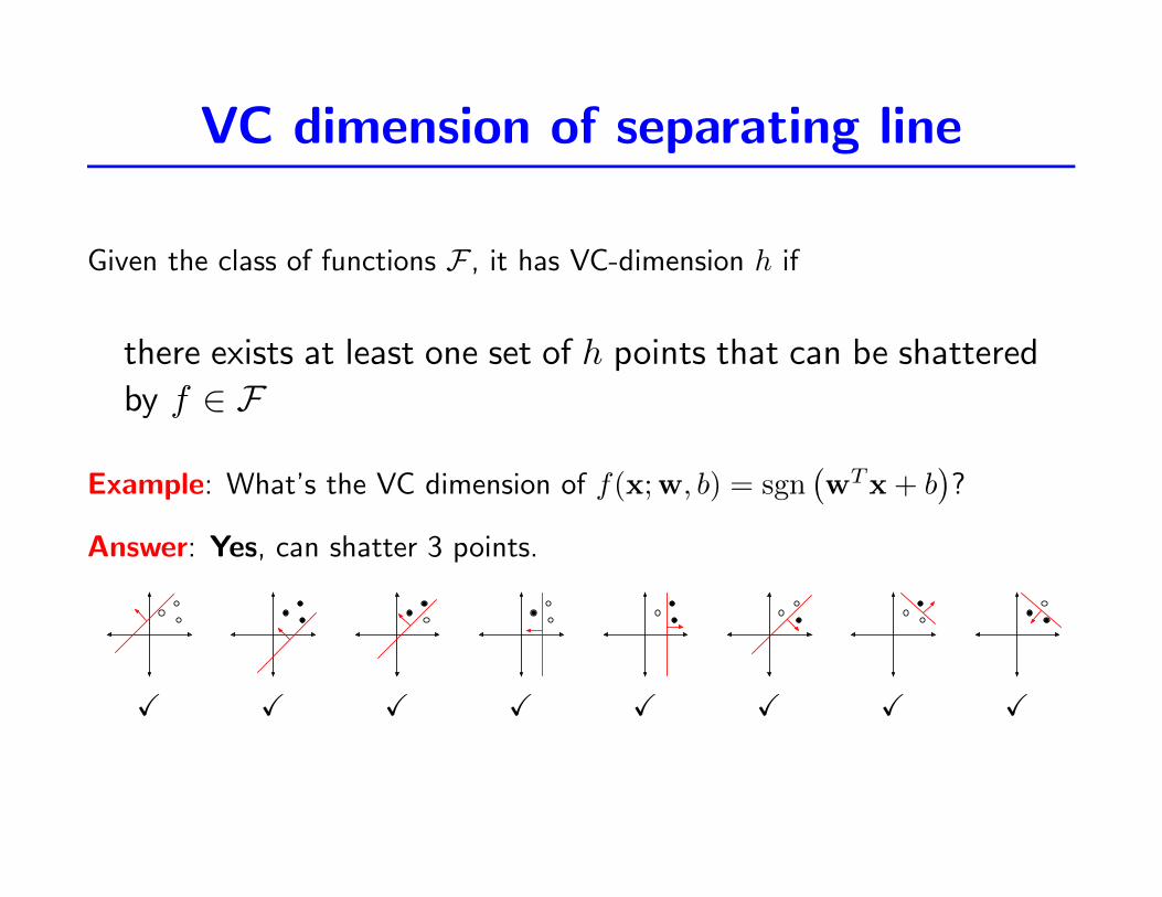
Example: What’s the VC dimension of f(x;w, b) = sgn(wTx + b
)?
Answer: Yes, can shatter 3 points.
X X X X X X X X
VC dimension of separating line
Given the class of functions F , it has VC-dimension h if
there exists at least one set of h points that can be shattered
by f ∈ F
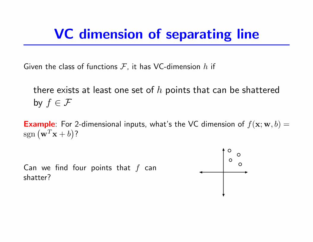
Example: For 2-dimensional inputs, what’s the VC dimension of f(x;w, b) =sgn
(wTx + b
)?
Can we find four points that f canshatter?
VC dimension of separating line
Given the class of functions F , it has VC-dimension h if
there exists at least one set of h points that can be shattered
by f ∈ F
Example: What’s the VC dimension of f(x;w, b) = sgn(wTx + b
)?
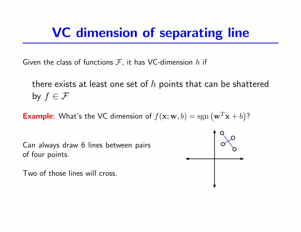
Can always draw 6 lines between pairsof four points.
VC dimension of separating line
Given the class of functions F , it has VC-dimension h if
there exists at least one set of h points that can be shattered
by f ∈ F
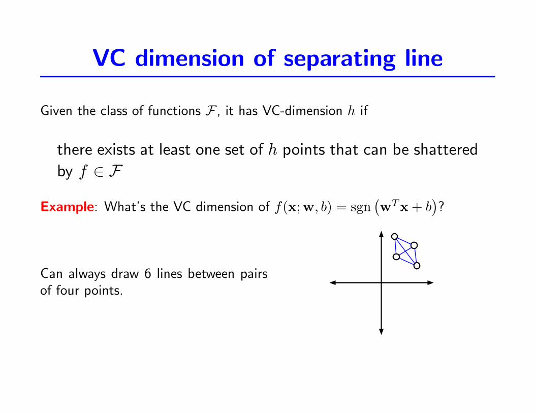
Example: What’s the VC dimension of f(x;w, b) = sgn(wTx + b
)?
Can always draw 6 lines between pairsof four points.
Two of those lines will cross.
VC dimension of separating line
Given the class of functions F , it has VC-dimension h if
there exists at least one set of h points that can be shattered by f ∈ F
Example: What’s the VC dimension of f(x;w, b) = sgn(wTx + b
)?
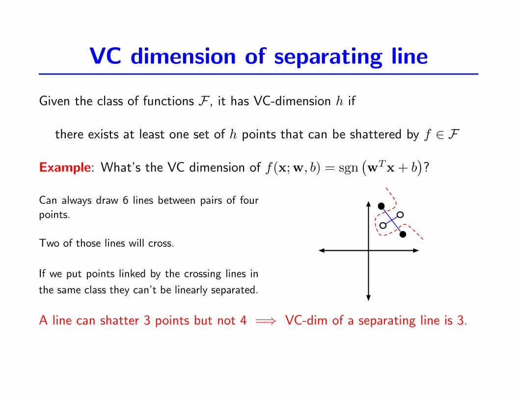
Can always draw 6 lines between pairs of four
points.
Two of those lines will cross.
If we put points linked by the crossing lines in
the same class they can’t be linearly separated.
A line can shatter 3 points but not 4 =⇒ VC-dim of a separating line is 3.
VC dimension of linear classifier in d-dimensions
If the input space is d-dimensional and if f is sgn(wTx− b
), what is its
VC-dimension?
Proof:
First will show d points can be shattered...
VC dimension of linear classifier in d-dimensions
If the input space is d-dimensional and if f is sgn(wTx− b
), what is its
VC-dimension?
Proof:
Define d input points thus:
x1 = (1, 0, 0, . . . , 0), x2 = (0, 1, 0, . . . , 0), . . . , xd = (0, 0, 0, . . . , 1)
So xk,j = 1 if k = j and 0 otherwise.
Let y1, y2, . . . , yd be any one of the 2d combinations of class labels.
How can we define w and b to ensure
sgn(wTxk + b
)= yk for all k ?
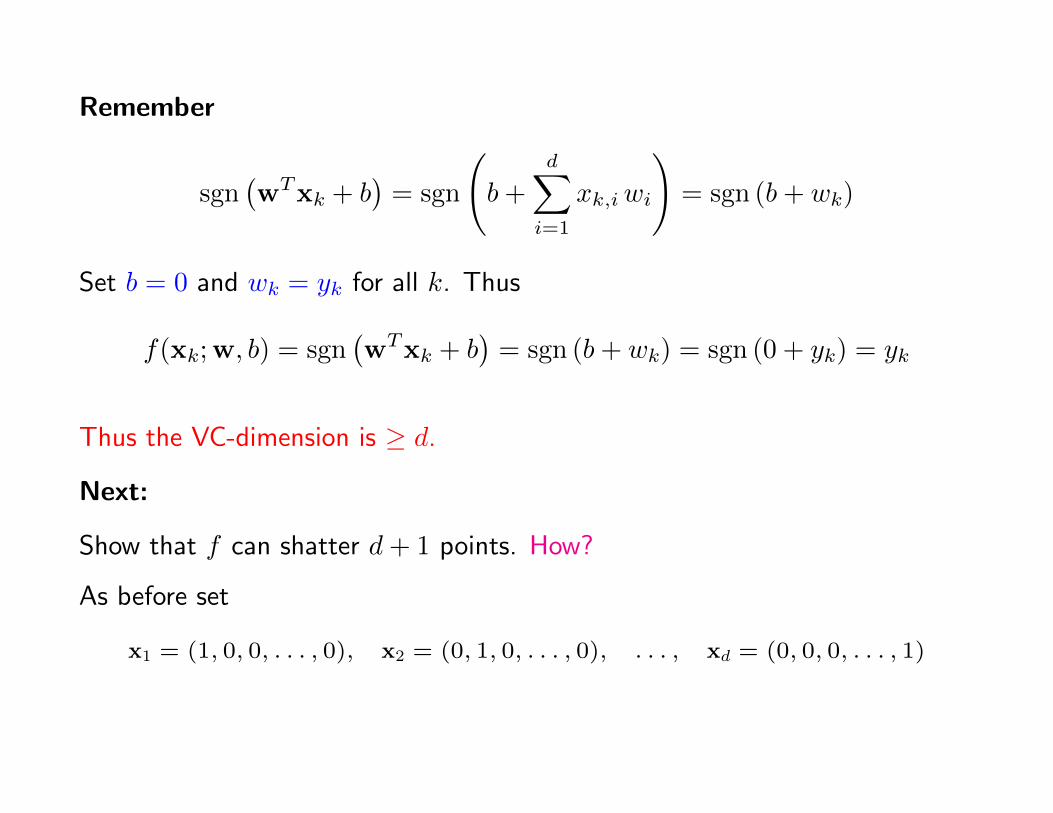
Remember
sgn(wTxk + b
)= sgn
(b+
d∑i=1
xk,iwi
)= sgn (b+ wk)
Set b = 0 and wk = yk for all k. Thus
f(xk;w, b) = sgn(wTxk + b
)= sgn (b+ wk) = sgn (0 + yk) = yk
Thus the VC-dimension is ≥ d.
Next:
Show that f can shatter d+ 1 points. How?
As before set
x1 = (1, 0, 0, . . . , 0), x2 = (0, 1, 0, . . . , 0), . . . , xd = (0, 0, 0, . . . , 1)
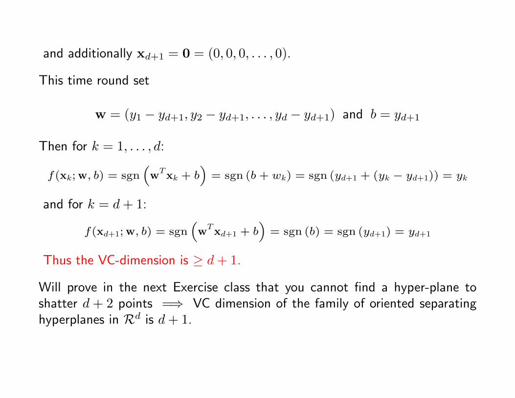
and additionally xd+1 = 0 = (0, 0, 0, . . . , 0).
This time round set
w = (y1 − yd+1, y2 − yd+1, . . . , yd − yd+1) and b = yd+1
Then for k = 1, . . . , d:
f(xk;w, b) = sgn(wTxk + b
)= sgn (b+ wk) = sgn (yd+1 + (yk − yd+1)) = yk
and for k = d+ 1:
f(xd+1;w, b) = sgn(wTxd+1 + b
)= sgn (b) = sgn (yd+1) = yd+1
Thus the VC-dimension is ≥ d+ 1.
Will prove in the next Exercise class that you cannot find a hyper-plane toshatter d + 2 points =⇒ VC dimension of the family of oriented separatinghyperplanes in Rd is d+ 1.
What does VC-dimension measure?
Is it the number of parameters?
Related but not really the same
One may intuitively expect that models with a large number of freeparameters would have high VC dimension, whereas models with fewparameters would have low VC dimensions.
However, consider this example....
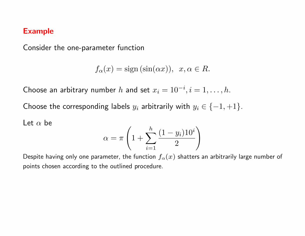
Example
Consider the one-parameter function
fα(x) = sign (sin(αx)), x, α ∈ R.
Choose an arbitrary number h and set xi = 10−i, i = 1, . . . , h.
Choose the corresponding labels yi arbitrarily with yi ∈ {−1,+1}.
Let α be
α = π
(1 +
h∑i=1
(1− yi)10i
2
)Despite having only one parameter, the function fα(x) shatters an arbitrarily large number of
points chosen according to the outlined procedure.
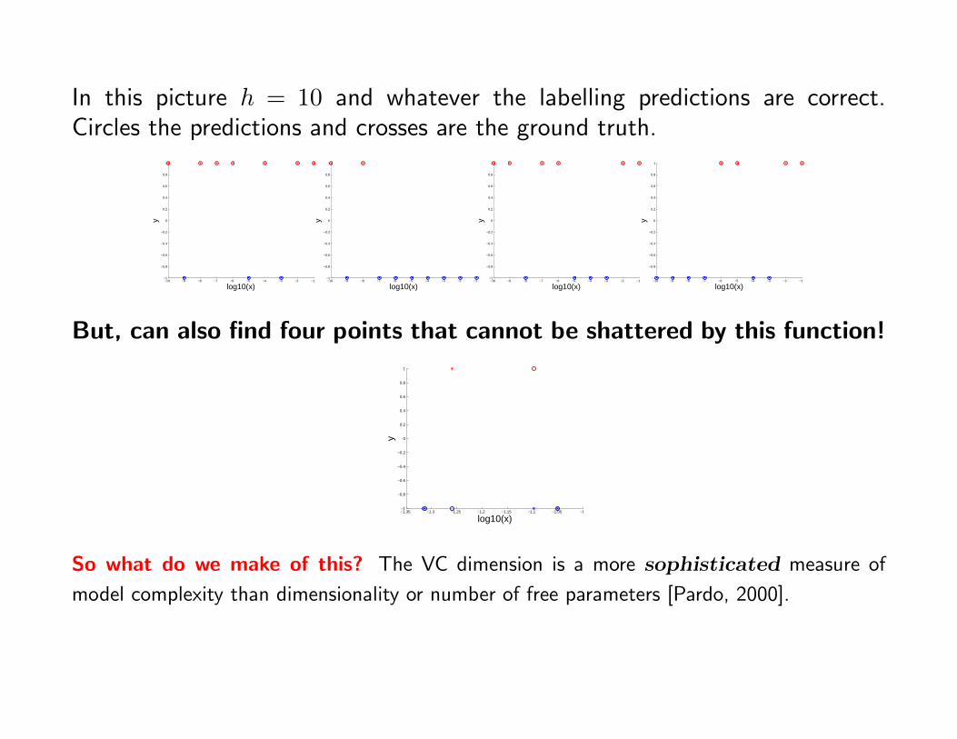
In this picture h = 10 and whatever the labelling predictions are correct.Circles the predictions and crosses are the ground truth.
−10 −9 −8 −7 −6 −5 −4 −3 −2 −1−1
−0.8
−0.6
−0.4
−0.2
0
0.2
0.4
0.6
0.8
1
log10(x)
y
−10 −9 −8 −7 −6 −5 −4 −3 −2 −1−1
−0.8
−0.6
−0.4
−0.2
0
0.2
0.4
0.6
0.8
1
log10(x)
y
−10 −9 −8 −7 −6 −5 −4 −3 −2 −1−1
−0.8
−0.6
−0.4
−0.2
0
0.2
0.4
0.6
0.8
1
log10(x)
y
−10 −9 −8 −7 −6 −5 −4 −3 −2 −1−1
−0.8
−0.6
−0.4
−0.2
0
0.2
0.4
0.6
0.8
1
log10(x)
y
But, can also find four points that cannot be shattered by this function!
−1.35 −1.3 −1.25 −1.2 −1.15 −1.1 −1.05 −1−1
−0.8
−0.6
−0.4
−0.2
0
0.2
0.4
0.6
0.8
1
log10(x)
y
So what do we make of this? The VC dimension is a more sophisticated measure of
model complexity than dimensionality or number of free parameters [Pardo, 2000].
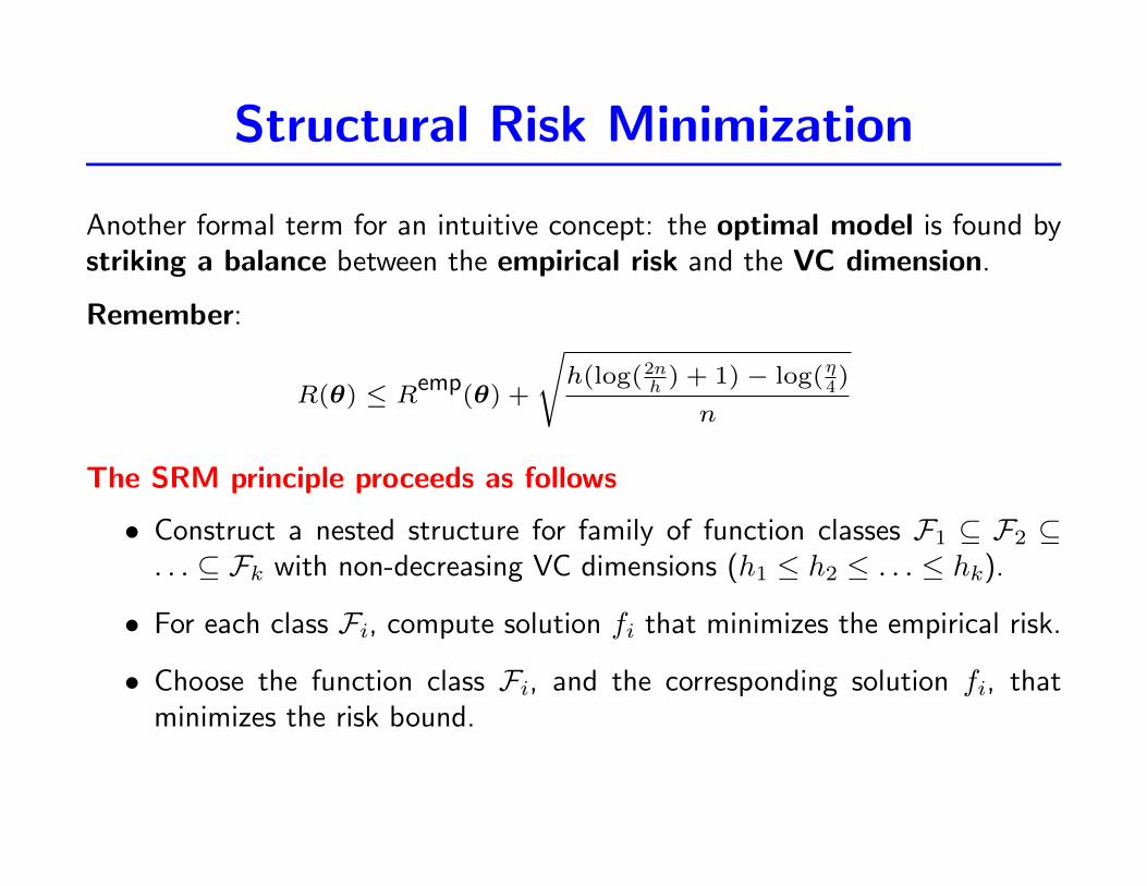
Structural Risk Minimization
Another formal term for an intuitive concept: the optimal model is found bystriking a balance between the empirical risk and the VC dimension.
Remember:
R(θ) ≤ Remp(θ) +
√h(log(2nh ) + 1)− log(η4)
n
The SRM principle proceeds as follows
• Construct a nested structure for family of function classes F1 ⊆ F2 ⊆. . . ⊆ Fk with non-decreasing VC dimensions (h1 ≤ h2 ≤ . . . ≤ hk).
• For each class Fi, compute solution fi that minimizes the empirical risk.
• Choose the function class Fi, and the corresponding solution fi, thatminimizes the risk bound.
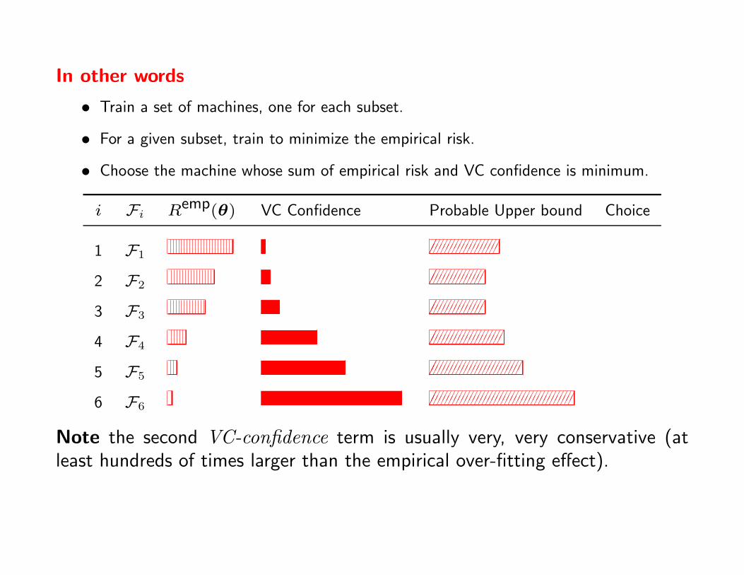
In other words
• Train a set of machines, one for each subset.
• For a given subset, train to minimize the empirical risk.
• Choose the machine whose sum of empirical risk and VC confidence is minimum.
i Fi Remp(θ) VC Confidence Probable Upper bound Choice
1 F1 H H H H H H H H H H H H H H H H H H H H H H H H H H H H H H H H H H H HH H
2 F2 H H H H H H H H H H H H H H H H H H H H H H H H H H H HH H
3 F3 H H H H H H H H H H H H H H H H H H H H H H H H H H H HH H
4 F4 H H H H H H H H H H H H H H H H H H H H H H H H H H H H H H H H H H H H H HH H
5 F5 H H H H H H H H H H H H H H H H H H H H H H H H H H H H H H H H H H H H H H H H H H H H H H H HH H
6 F6 H H H H H H H H H H H H H H H H H H H H H H H H H H H H H H H H H H H H H H H H H H H H H H H H H H H H H H H H H H H H H H H H H H H H H H H H H H H HH HNote the second VC-confidence term is usually very, very conservative (atleast hundreds of times larger than the empirical over-fitting effect).
Structural Risk Minimization
Introduction to Pattern AnalysisRicardo Gutierrez-OsunaTexas A&M University
10
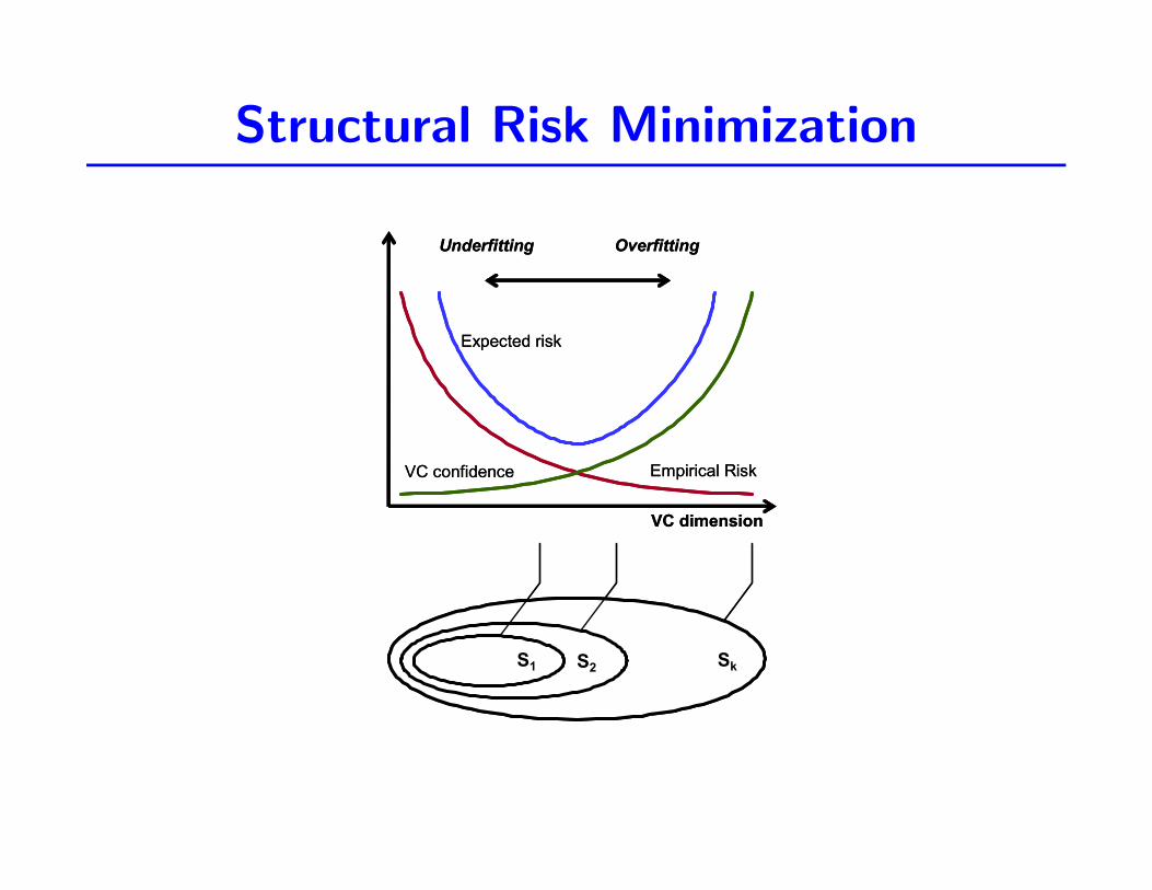
Structural Risk Minimization (3)
From [Cherkassky and Mulier, 1998]
VC dimension
Empirical RiskVC confidence
Expected risk
SkS1 S2
Underfitting Overfitting
VC dimension
Empirical RiskVC confidence
Expected risk
SkS1 S2
Underfitting Overfitting
Using VC-dimensionality
People have worked hard to find the VC-dimension for
• Perceptrons
• Neural Nets
• Support Vector Machines
• And many many more
All with the goals of
1. Understanding which learning machines are more or less powerful underwhich circumstances.
2. Using Structural Risk Minimization to choose the best learning machine.
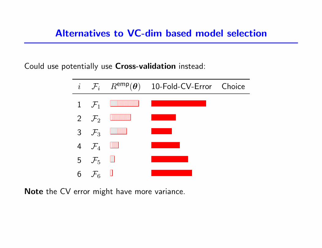
Alternatives to VC-dim based model selection
Could use potentially use Cross-validation instead:
i Fi Remp(θ) 10-Fold-CV-Error Choice
1 F1
2 F2
3 F3
4 F4
5 F5
6 F6
Note the CV error might have more variance.
The VC dimension in practice
Unfortunately, computing an upper bound on the expected risk is notpractical in various situations
• The VC dimension cannot be accurately estimated for non-linear modelssuch as neural networks.
• Implementation of Structural Risk Minimization may lead to a non-linearoptimization problem.
• The VC dimension may be infinite (e.g., k = 1 nearest neighbor),requiring infinite amount of data.
• The upper bound may sometimes be trivial (e.g., larger than one).
Fortunately, Statistical Learning Theory can be rigorously applied in therealm of linear models.
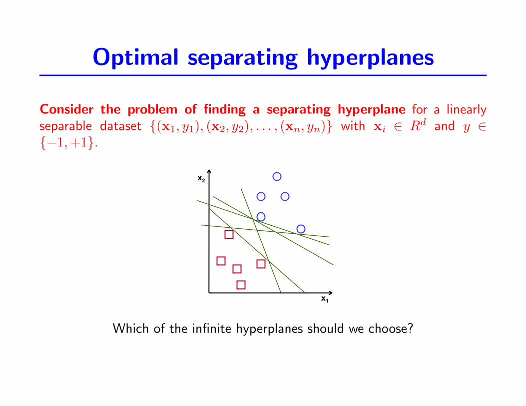
Optimal separating hyperplanes
Consider the problem of finding a separating hyperplane for a linearlyseparable dataset {(x1, y1), (x2, y2), . . . , (xn, yn)} with xi ∈ Rd and y ∈{−1,+1}.
Introduction to Pattern AnalysisRicardo Gutierrez-OsunaTexas A&M University
12
Optimal separating hyperplanes (1)! Consider the problem of finding a separating hyperplane for a linearly
separable dataset {(x1,y1),(x2,y2),…,(xN,yN)}, x!RD, y!{-1,+1}" Which of the infinite hyperplanes should we choose?
! Intuitively, a hyperplane that passes too close to the training examples will be sensitive to noise and, therefore, less likely to generalize well for data outside the training set
! Instead, it seems reasonable to expect that a hyperplane that is farthest from all training examples will have better generalization capabilities
" Therefore, the optimal separating hyperplane will be the one with the largest margin, which is defined as the minimum distance of an example to the decision surface
From [Cherkassky and Mulier, 1998]
x1
x2
x1
x2
Optimal hyperplane
Maximummargin
Which of the infinite hyperplanes should we choose?
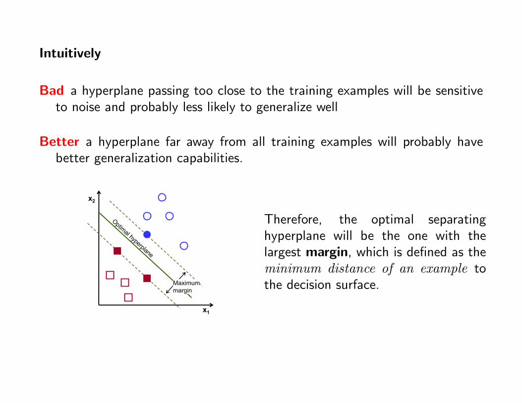
Intuitively
Bad a hyperplane passing too close to the training examples will be sensitiveto noise and probably less likely to generalize well
Better a hyperplane far away from all training examples will probably havebetter generalization capabilities.
Introduction to Pattern AnalysisRicardo Gutierrez-OsunaTexas A&M University
12
Optimal separating hyperplanes (1)! Consider the problem of finding a separating hyperplane for a linearly
separable dataset {(x1,y1),(x2,y2),…,(xN,yN)}, x!RD, y!{-1,+1}" Which of the infinite hyperplanes should we choose?
! Intuitively, a hyperplane that passes too close to the training examples will be sensitive to noise and, therefore, less likely to generalize well for data outside the training set
! Instead, it seems reasonable to expect that a hyperplane that is farthest from all training examples will have better generalization capabilities
" Therefore, the optimal separating hyperplane will be the one with the largest margin, which is defined as the minimum distance of an example to the decision surface
From [Cherkassky and Mulier, 1998]
x1
x2
x1
x2
Optimal hyperplane
Maximummargin
Therefore, the optimal separatinghyperplane will be the one with thelargest margin, which is defined as theminimum distance of an example tothe decision surface.
Optimal separating hyperplanes
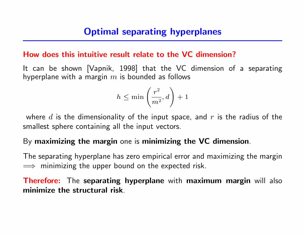
How does this intuitive result relate to the VC dimension?
It can be shown [Vapnik, 1998] that the VC dimension of a separatinghyperplane with a margin m is bounded as follows
h ≤ min
(r2
m2, d
)+ 1
where d is the dimensionality of the input space, and r is the radius of thesmallest sphere containing all the input vectors.
By maximizing the margin one is minimizing the VC dimension.
The separating hyperplane has zero empirical error and maximizing the margin=⇒ minimizing the upper bound on the expected risk.
Therefore: The separating hyperplane with maximum margin will alsominimize the structural risk.
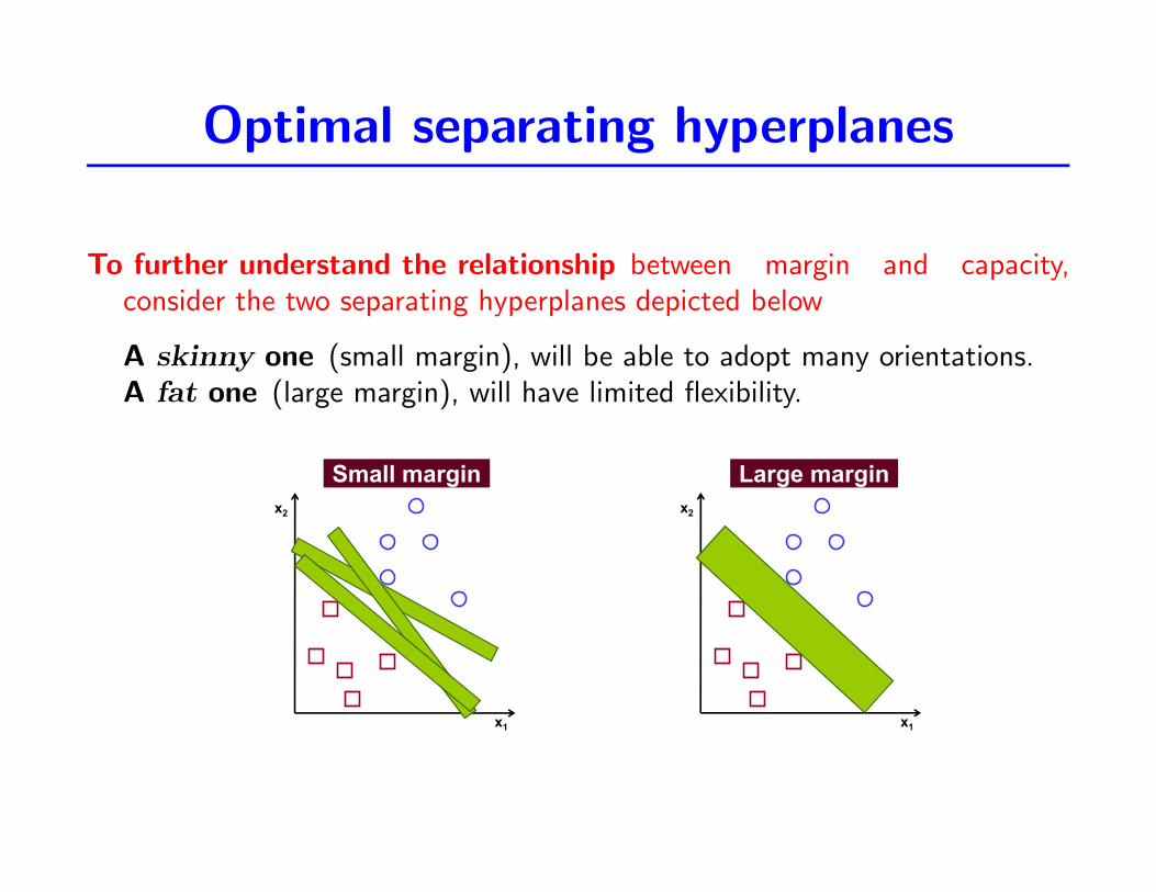
Optimal separating hyperplanes
To further understand the relationship between margin and capacity,consider the two separating hyperplanes depicted below
A skinny one (small margin), will be able to adopt many orientations.A fat one (large margin), will have limited flexibility.
Introduction to Pattern AnalysisRicardo Gutierrez-OsunaTexas A&M University
14
Optimal separating hyperplanes (3)! To further understand the relationship between margin and capacity,
consider the two separating hyperplanes depicted below" A “skinny” one (small margin), which will be able to adopt many orientations" A “fat” one (large margin), which will have limited flexibility
! A larger margin necessarily results in lower capacity" We normally think of complexity as being a function of the number of parameters
! Instead, Statistical Learning Theory tells us that if the margin is sufficiently large, the complexity of the function will be low even if the dimensionality is very high!
From [Bennett and Campbell, 2000]
x1
x2
Small margin Large margin
x1
x2
A larger margin necessarily results in lower capacity
• We normally think of complexity as being a function of the number ofparameters.
Instead, Statistical Learning Theory tells us that if the margin issufficiently large, the complexity of the function will be low evenif the dimensionality is very high!
Optimal separating hyperplanes
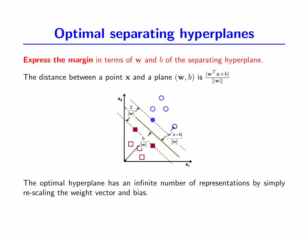
Express the margin in terms of w and b of the separating hyperplane.
The distance between a point x and a plane (w, b) is |wTx+b|‖w‖
Introduction to Pattern AnalysisRicardo Gutierrez-OsunaTexas A&M University
15
Optimal separating hyperplanes (4)! Since we want to maximize the margin, let’s express it as a function of
the weight vector and bias of the separating hyperplane" From basic trigonometry, the distance between a point x and a plane (w,b) is
" Noticing that the optimal hyperplane has infinite solutions by simply scaling the weight vector and bias, we choose the solution for which the discriminant function becomes one for the training examples closest to the boundary
! This is known as the canonical hyperplane" Therefore, the distance from the closest
example to the boundary is
" And the margin becomes
wbxwT !
1bxw iT "!
w1
wbxwT
"!
w2m "
x1
x2
wbxwT !
wb
w2
x1
x2
wbxwT !
wb
w2
The optimal hyperplane has an infinite number of representations by simplyre-scaling the weight vector and bias.
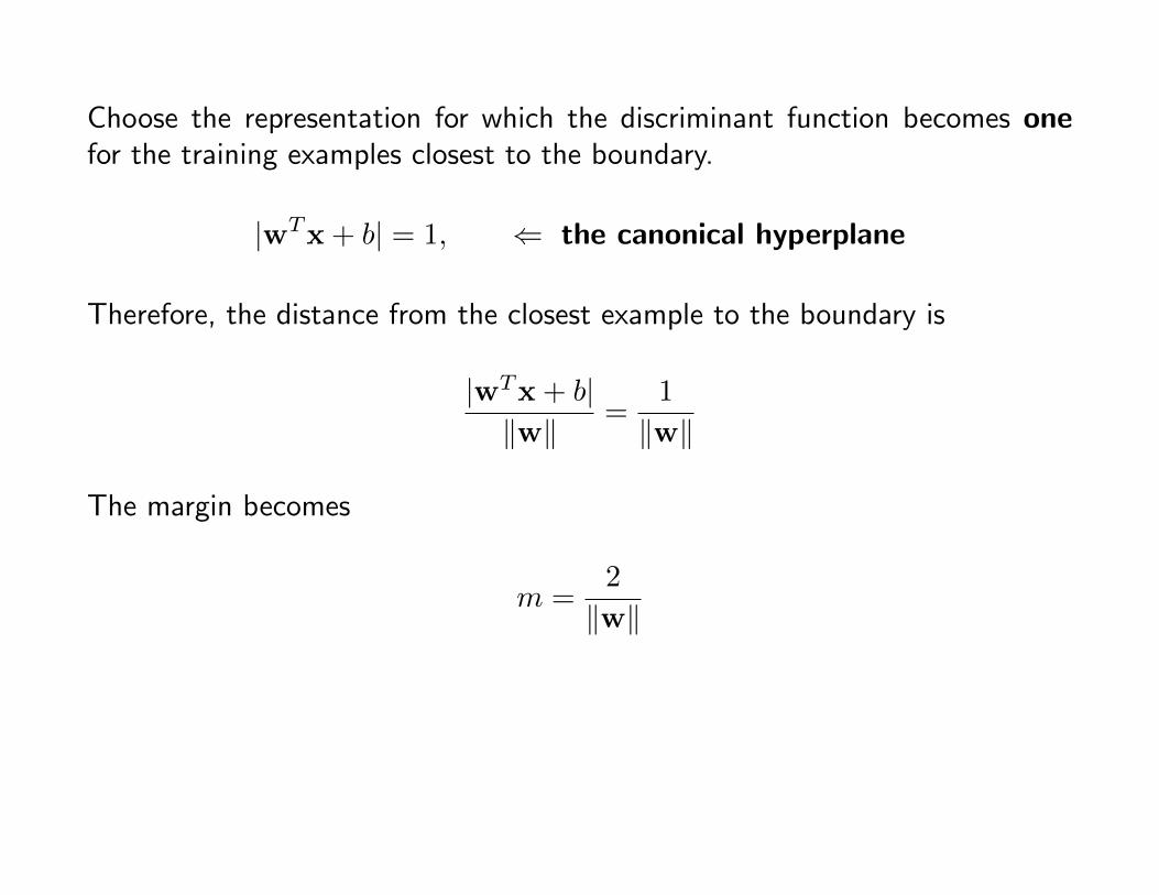
Choose the representation for which the discriminant function becomes onefor the training examples closest to the boundary.
|wTx + b| = 1, ⇐ the canonical hyperplane
Therefore, the distance from the closest example to the boundary is
|wTx + b|‖w‖
=1
‖w‖
The margin becomes
m =2
‖w‖
Optimal separating hyperplanes
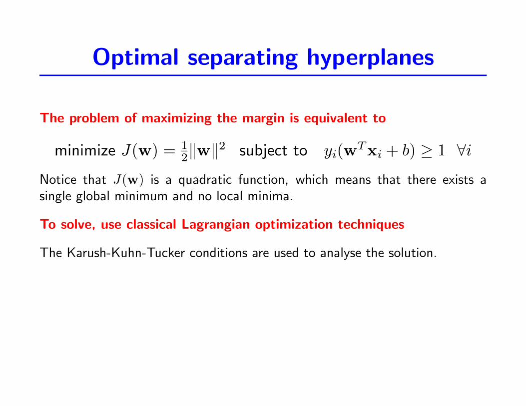
The problem of maximizing the margin is equivalent to
minimize J(w) = 12‖w‖
2 subject to yi(wTxi + b) ≥ 1 ∀i
Notice that J(w) is a quadratic function, which means that there exists asingle global minimum and no local minima.
To solve, use classical Lagrangian optimization techniques
The Karush-Kuhn-Tucker conditions are used to analyse the solution.
Lagrange multipliers
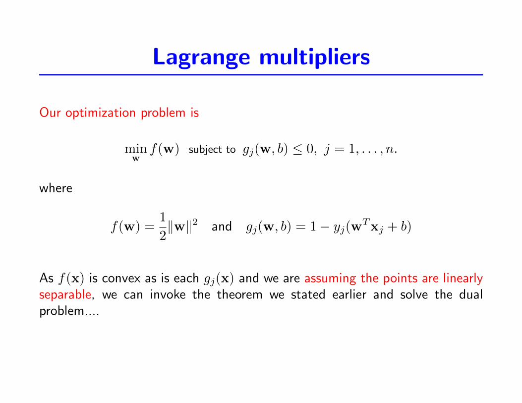
Our optimization problem is
minwf(w) subject to gj(w, b) ≤ 0, j = 1, . . . , n.
where
f(w) =1
2‖w‖2 and gj(w, b) = 1− yj(wTxj + b)
As f(x) is convex as is each gj(x) and we are assuming the points are linearlyseparable, we can invoke the theorem we stated earlier and solve the dualproblem....
Properties of the solution
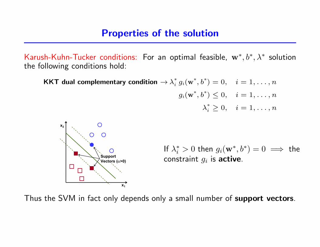
Karush-Kuhn-Tucker conditions: For an optimal feasible, w∗, b∗, λ∗ solutionthe following conditions hold:
KKT dual complementary condition →λ∗i gi(w
∗, b∗) = 0, i = 1, . . . , n
gi(w∗, b∗) ≤ 0, i = 1, . . . , n
λ∗i ≥ 0, i = 1, . . . , n
Introduction to Pattern AnalysisRicardo Gutierrez-OsunaTexas A&M University
22
Support Vectors! The KTT complementary condition states that, for every point in the
training set, the following equality must hold
" Therefore, for each example, either !i=0 or yi(wTxi+b-1)=0 must hold" Those points for which !i>0 must then lie on one of the two hyperplanes that
define the largest margin (only at these hyperplanes the term yi(wTxi+b-1) becomes zero)
! These points are known as the Support Vectors" All the other points must have !i=0 " Note that only the support vectors contribute
to defining the optimal hyperplane
! NOTE: the bias term b is found from the KKTcomplementary condition on the support vectors
" Therefore, the complete dataset could be replaced by only the support vectors, and the separating hyperplane would be the same
" #$ % 1...Ni01bxwy! iT
ii &'&()
" # *&
&+&,
, N
1iiii xy!w0
w!b,w,J
x1
x2
Support Vectors (!>0)
If λ∗i > 0 then gi(w∗, b∗) = 0 =⇒ the
constraint gi is active.
Thus the SVM in fact only depends only a small number of support vectors.
The dual problem
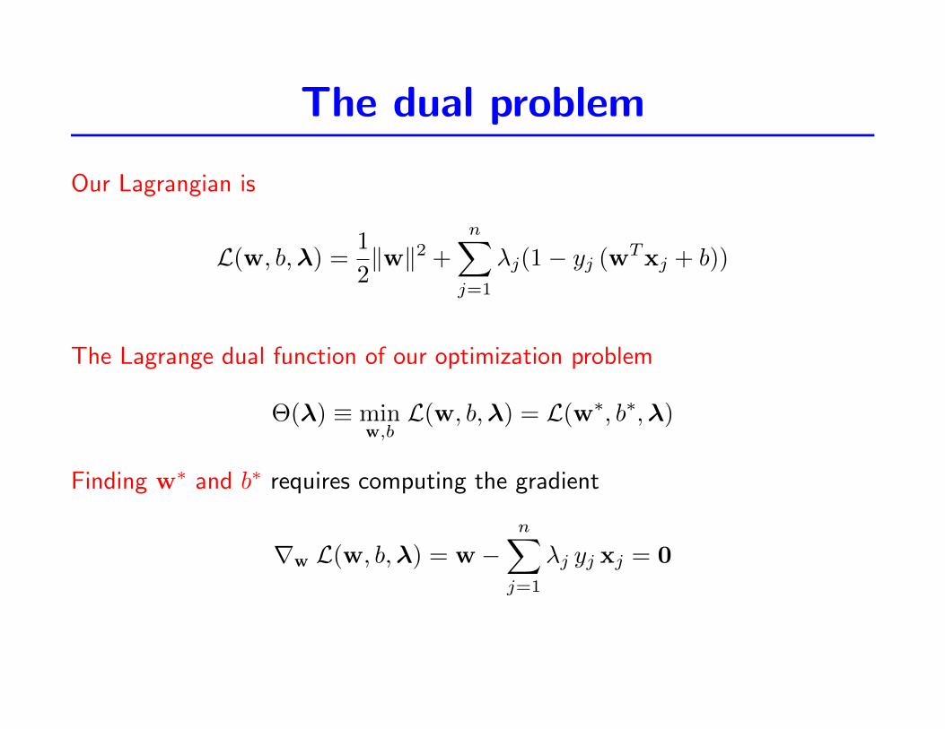
Our Lagrangian is
L(w, b,λ) =1
2‖w‖2 +
n∑j=1
λj(1− yj (wTxj + b))
The Lagrange dual function of our optimization problem
Θ(λ) ≡ minw,bL(w, b,λ) = L(w∗, b∗,λ)
Finding w∗ and b∗ requires computing the gradient
∇w L(w, b,λ) = w −n∑j=1
λj yj xj = 0
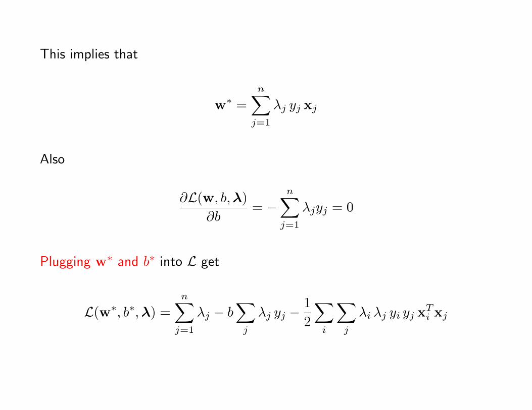
This implies that
w∗ =
n∑j=1
λj yj xj
Also
∂L(w, b,λ)
∂b= −
n∑j=1
λjyj = 0
Plugging w∗ and b∗ into L get
L(w∗, b∗,λ) =
n∑j=1
λj − b∑j
λj yj −1
2
∑i
∑j
λi λj yi yj xTi xj
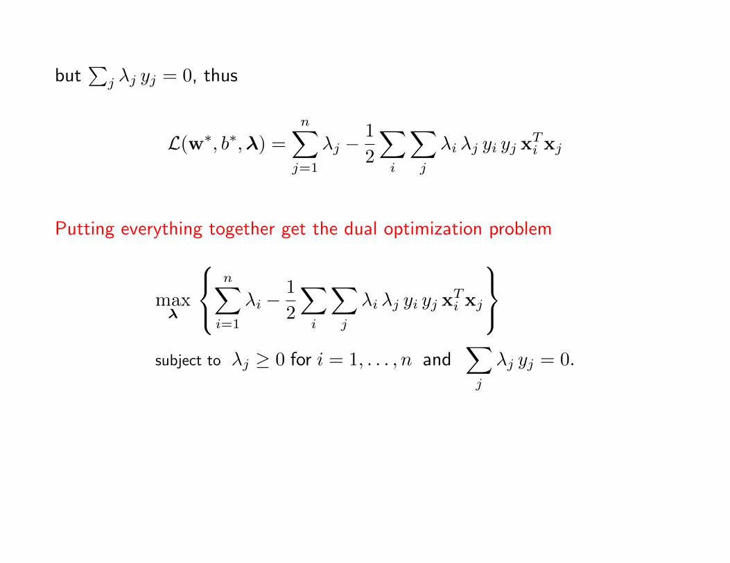
but∑j λj yj = 0, thus
L(w∗, b∗,λ) =
n∑j=1
λj −1
2
∑i
∑j
λi λj yi yj xTi xj
Putting everything together get the dual optimization problem
maxλ
n∑i=1
λi −1
2
∑i
∑j
λi λj yi yj xTi xj
subject to λj ≥ 0 for i = 1, . . . , n and
∑j
λj yj = 0.
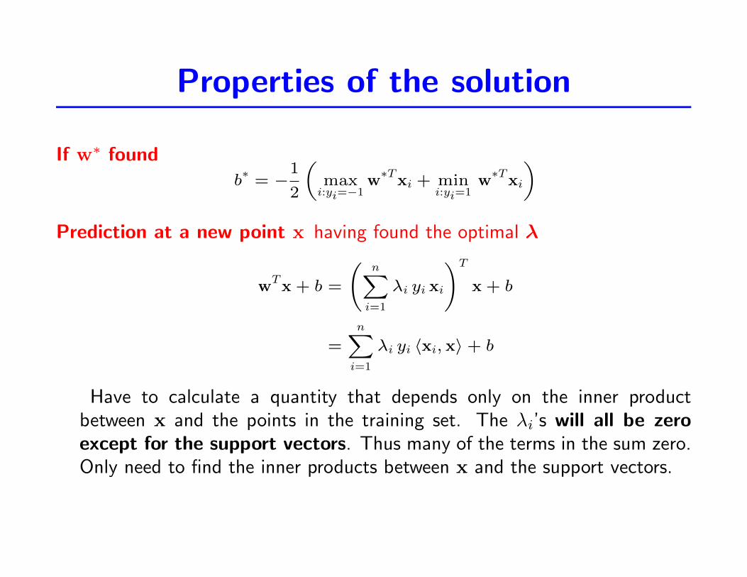
Properties of the solution
If w∗ foundb∗= −
1
2
(maxi:yi=−1
w∗T
xi + mini:yi=1
w∗T
xi
)Prediction at a new point x having found the optimal λ
wTx + b =
(n∑i=1
λi yi xi
)T
x + b
=
n∑i=1
λi yi 〈xi, x〉+ b
Have to calculate a quantity that depends only on the inner productbetween x and the points in the training set. The λi’s will all be zeroexcept for the support vectors. Thus many of the terms in the sum zero.Only need to find the inner products between x and the support vectors.

Pen & Paper assignment
• Details available on the course website.
• Your assignment is a small pen & paper exercise based on hand calculationof a separating line.
• Mail me about any errors you spot in the Exercise notes.
• I will notify the class about errors spotted and corrections via the coursewebsite and mailing list.


![arXiv:2004.06051v2 [math.DG] 21 Apr 20202 HENRIK MATTHIESEN AND ROMAIN PETRIDES Notice that in our result, the dimension of the target ball is controlled by the multiplicity of the](https://static.fdocument.org/doc/165x107/60bbf896c0bd6d459711f2bd/arxiv200406051v2-mathdg-21-apr-2020-2-henrik-matthiesen-and-romain-petrides.jpg)