6.003: Signals and Systems

Frequency Response

October 6, 2011 1

Review

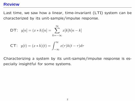
Last time, we saw how a linear, time-invariant (LTI) system can be

characterized by its unit-sample/impulse response.

∞0 DT: y[n] = (x ∗ h)[n] = x[k]h[n − k]

k=−∞ � ∞ CT: y(t) = (x ∗ h)(t) = x(τ)h(t − τ)dτ

−∞

Characterizing a system by its unit-sample/impulse response is es­

pecially insightful for some systems.

2

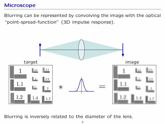
Microscope

Blurring can be represented by convolving the image with the optical

“point-spread-function” (3D impulse response).

Blurring is inversely related to the diameter of the lens.

target image

∗ =

3

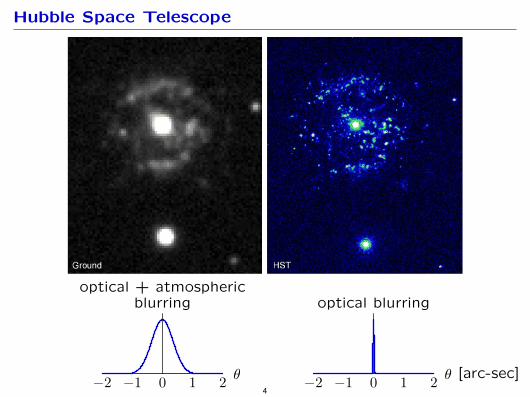
Hubble Space Telescope

−2 −1 0 1 2 θ

optical + atmosphericblurring

−2 −1 0 1 2 θ

optical blurring

[arc-sec]4

Frequency Response

Today we will investigate a different way to characterize a system:

the frequency response.

Many systems are naturally described by their responses to sinusoids.

Example: audio systems

5

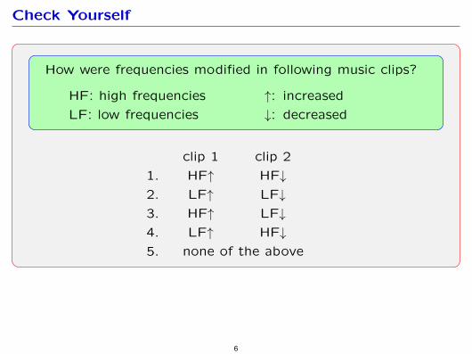
Check Yourself

How were frequencies modified in following music clips?

HF: high frequencies ↑: increased

LF: low frequencies ↓: decreased

clip 1 clip 2

1. HF↑ HF↓

2. LF↑ LF↓

3. HF↑ LF↓

4. LF↑ HF↓

5. none of the above

6

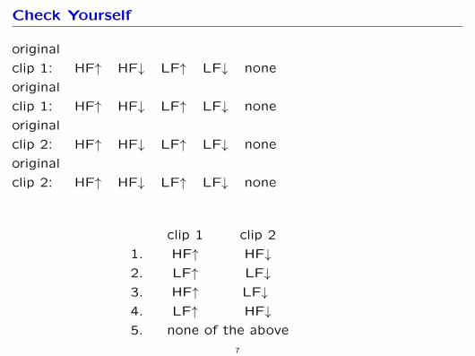
Check Yourself

original

clip 1: HF↑ HF↓

original

clip 1: HF↑ HF↓

original

clip 2: HF↑ HF↓

original

clip 2: HF↑ HF↓

1.

2.

3.

4.

5.

LF↑ LF↓ none

LF↑ LF↓ none

LF↑ LF↓ none

LF↑ LF↓ none

clip 1 clip 2

HF↑ HF↓

LF↑ LF↓

HF↑ LF↓

LF↑ HF↓

none of the above

7

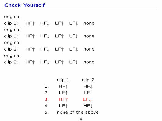
Check Yourself

original

clip 1: HF↑ HF↓

original

clip 1: HF↑ HF↓

original

clip 2: HF↑ HF↓

original

clip 2: HF↑ HF↓

1.

2.

3.

4.

5.

LF↑ LF↓ none

LF↑ LF↓ none

LF↑ LF↓ none

LF↑ LF↓ none

clip 1 clip 2

HF↑ HF↓

LF↑ LF↓

HF↑ LF↓

LF↑ HF↓

none of the above

8

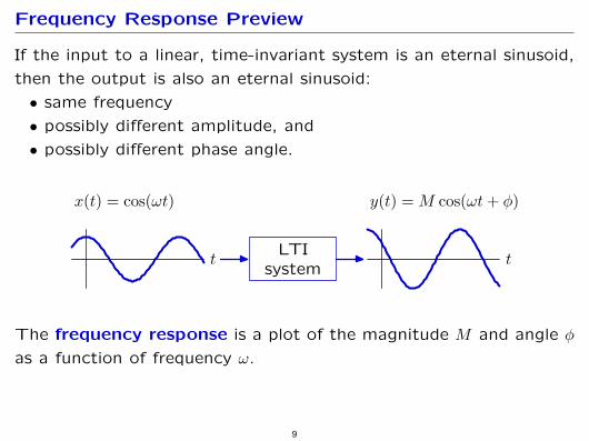
Frequency Response Preview

If the input to a linear, time-invariant system is an eternal sinusoid,

then the output is also an eternal sinusoid:

• same frequency

• possibly different amplitude, and

• possibly different phase angle.

The frequency response is a plot of the magnitude M and angle φ

as a function of frequency ω.

x(t) = cos(ωt)

t

y(t) = M cos(ωt+ φ)

tLTI

system

9

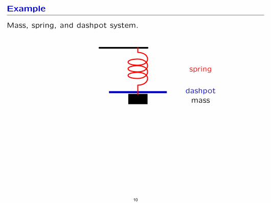
Example

Mass, spring, and dashpot system.

spring

dashpotmass

10

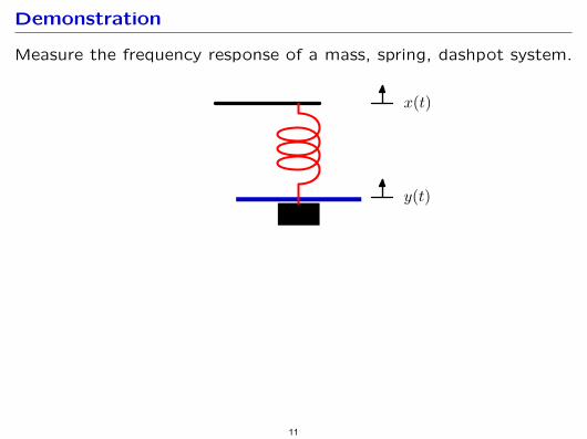
Demonstration

Measure the frequency response of a mass, spring, dashpot system.

x(t)

y(t)

11

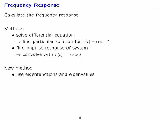
Frequency Response

Calculate the frequency response.

Methods

• solve differential equation

→ find particular solution for x(t) = cos ω0t

• find impulse response of system

→ convolve with x(t) = cos ω0t

New method

• use eigenfunctions and eigenvalues

12

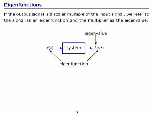
Eigenfunctions

If the output signal is a scalar multiple of the input signal, we refer to

the signal as an eigenfunction and the multiplier as the eigenvalue.

systemx(t) λx(t)

eigenvalue

eigenfunction

13

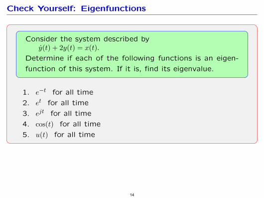
Check Yourself: Eigenfunctions

Consider the system described by y(t) + 2y(t) = x(t).

Determine if each of the following functions is an eigen­

function of this system. If it is, find its eigenvalue.

1. e−t for all time

2. et for all time

3. ejt for all time

4. cos(t) for all time

5. u(t) for all time

14

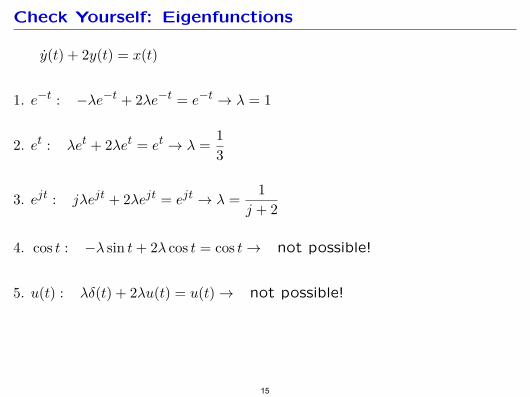
Check Yourself: Eigenfunctions

y(t) + 2y(t) = x(t)

−t :1. e −λe−t + 2λe−t = e −t → λ = 1

12. e t : λet + 2λet = e t → λ = 3

1jt : jt → λ =3. e jλejt + 2λejt = ej + 2

4. cos t : −λ sin t + 2λ cos t = cos t → not possible!

5. u(t) : λδ(t) + 2λu(t) = u(t) → not possible!

15

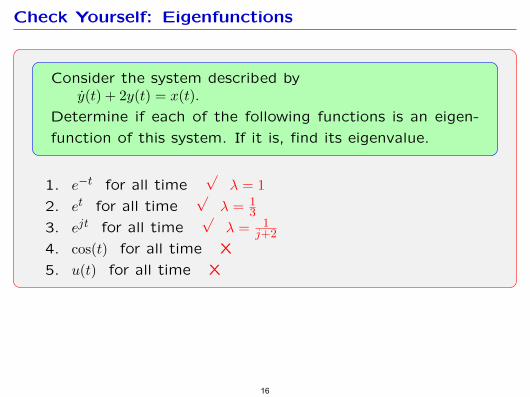
Check Yourself: Eigenfunctions

Consider the system described by y(t) + 2y(t) = x(t).

Determine if each of the following functions is an eigen­

function of this system. If it is, find its eigenvalue.

1. e−t for all time √

λ = 1

2. et for all time √

λ = 1 3

3. ejt for all time √

λ = 1 j+2

4. cos(t) for all time X

5. u(t) for all time X

16

� �

� �

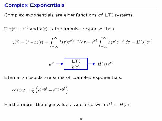
Complex Exponentials

Complex exponentials are eigenfunctions of LTI systems.

stIf x(t) = e and h(t) is the impulse response then

∞ ∞ st st y(t) = (h ∗ x)(t) = h(τ )e s(t−τ)dτ = e h(τ)e −sτ dτ = H(s) e

−∞ −∞

est H(s) estLTIh(t)

Eternal sinusoids are sums of complex exponentials.

1 jω0t + e −jω0tcos ω0t = e2

stFurthermore, the eigenvalue associated with e is H(s) !

17

∫ ∫

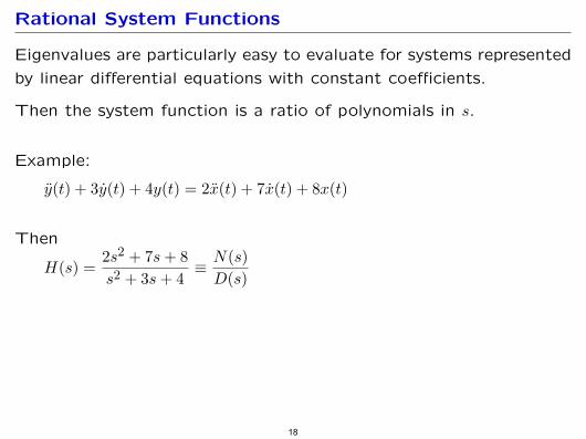
Rational System Functions

Eigenvalues are particularly easy to evaluate for systems represented

by linear differential equations with constant coefficients.

Then the system function is a ratio of polynomials in s.

Example:

y(t) + 3y(t) + 4y(t) = 2x(t) + 7x(t) + 8x(t)

Then 2s2 + 7s + 8 N(s)

H(s) = ≡ s2 + 3s + 4 D(s)

18

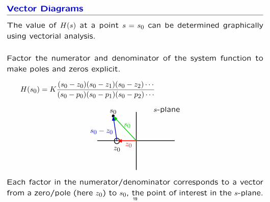
Vector Diagrams

The value of H(s) at a point s = s0 can be determined graphically

using vectorial analysis.

Factor the numerator and denominator of the system function to

make poles and zeros explicit.

(s0 − z0)(s0 − z1)(s0 − z2) · · · H(s0) = K (s0 − p0)(s0 − p1)(s0 − p2) · · ·

z0z0

s0 − z0s0

s-planes0

Each factor in the numerator/denominator corresponds to a vector

from a zero/pole (here z0) to s0, the point of interest in the s-plane. 19

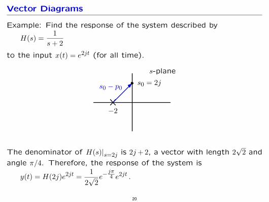
Vector Diagrams

Example: Find the response of the system described by 1

H(s) = s + 2

to the input x(t) = e2jt (for all time).

−2

s0 − p0

s-plane

s0 = 2j

√The denominator of H(s)|s=2j is 2j + 2, a vector with length 2 2 and

angle π/4. Therefore, the response of the system is 1 jπ2jt − 2jt y(t) = H(2j)e = √ e 4 e .

2 2

20

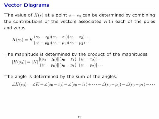
Vector Diagrams

The value of H(s) at a point s = s0 can be determined by combining

the contributions of the vectors associated with each of the poles

and zeros.

(s0 − z0)(s0 − z1)(s0 − z2) · · · H(s0) = K (s0 − p0)(s0 − p1)(s0 − p2) · · ·

The magnitude is determined by the product of the magnitudes. |(s0 − z0)||(s0 − z1)||(s0 − z2)| · · · |H(s0)| = |K||(s0 − p0)||(s0 − p1)||(s0 − p2)| · · ·

The angle is determined by the sum of the angles.

∠H(s0) = ∠K + ∠(s0 − z0)+ ∠(s0 − z1)+ · · ·− ∠(s0 − p0) − ∠(s0 − p1) −· · ·

21

� �

� �

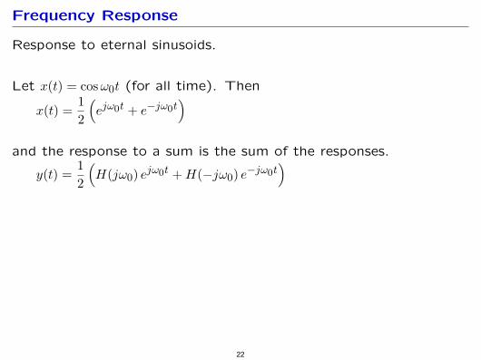
Frequency Response

Response to eternal sinusoids.

Let x(t) = cos ω0t (for all time). Then 1 jω0t + e −jω0t x(t) = e2

and the response to a sum is the sum of the responses. 1 jω0t + H(−jω0) e −jω0t y(t) = H(jω0) e2

22

( )

( )

�

��

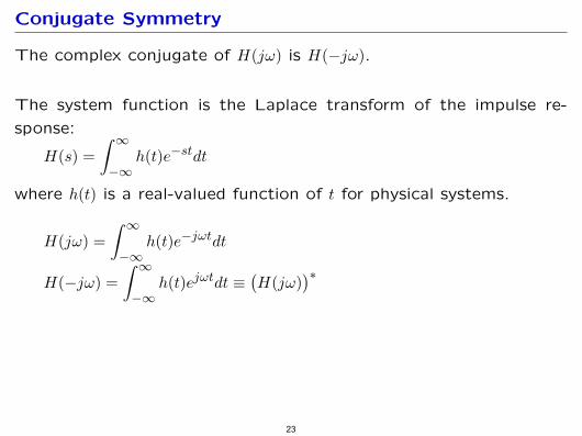
Conjugate Symmetry

The complex conjugate of H(jω) is H(−jω).

The system function is the Laplace transform of the impulse re­

sponse: ∞

H(s) = h(t)e −stdt −∞

where h(t) is a real-valued function of t for physical systems.

∞ −jωtdtH(jω) = h(t)e

−∞ ∞

jωtdt ≡H(−jω) = h(t)e H(jω)

∗

−∞

23

∫

∫∫

� �

� �

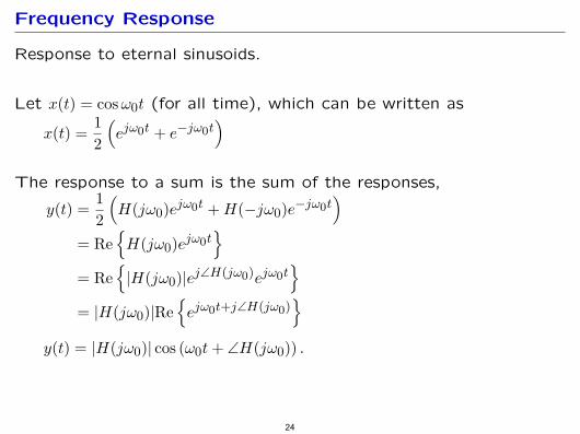
Frequency Response

Response to eternal sinusoids.

Let x(t) = cos ω0t (for all time), which can be written as 1 jω0t + e −jω0t x(t) = e2

The response to a sum is the sum of the responses, 1 −jω0t y(t) = H(jω0)ejω0t + H(−jω0)e2

= Re H(jω0)ejω0t = Re |H(jω0)|ej∠H(jω0)ejω0t = |H(jω0)|Re ejω0t+j∠H(jω0)

y(t) = |H(jω0)| cos (ω0t + ∠H(jω0)) .

24

( )

( )

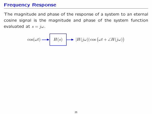
Frequency Response

The magnitude and phase of the response of a system to an eternal

cosine signal is the magnitude and phase of the system function

evaluated at s = jω.

H(s)cos(ωt) |H(jω)| cos(ωt+ ∠H(jω)

)

25

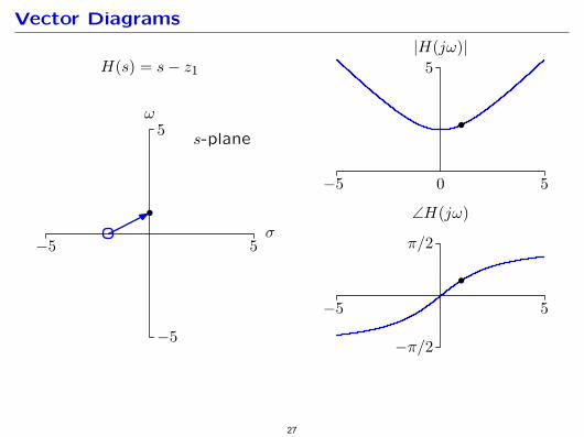
Vector Diagrams

s-plane

σ

ω5

−5

5−5

H(s) = s− z1

−5 0 5

5|H(jω)|

−5 5

π/2

−π/2

∠H(jω)

26

s-plane

σ

ω5

−5

5−5

H(s) = s− z1

−5 0 5

5|H(jω)|

−5 5

π/2

−π/2

∠H(jω)

Vector Diagrams

27

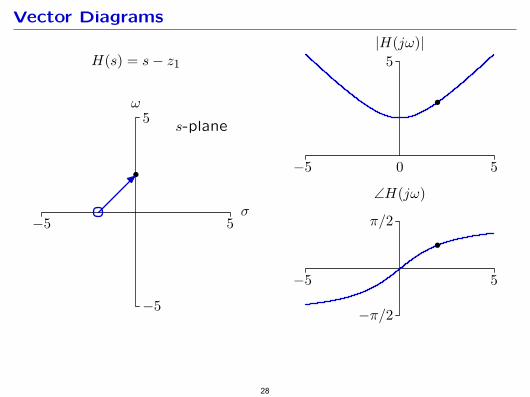
Vector Diagrams

s-plane

σ

ω5

−5

5−5

H(s) = s− z1

−5 0 5

5|H(jω)|

−5 5

π/2

−π/2

∠H(jω)

28

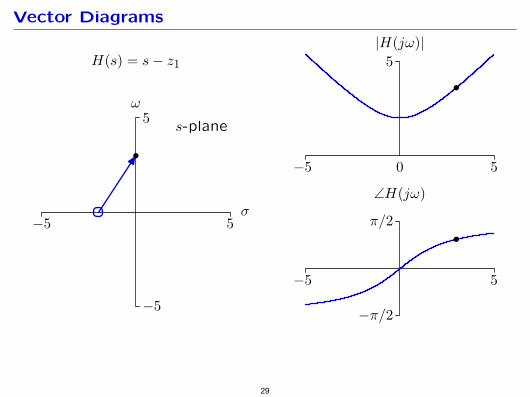
Vector Diagrams

s-plane

σ

ω5

−5

5−5

H(s) = s− z1

−5 0 5

5|H(jω)|

−5 5

π/2

−π/2

∠H(jω)

29

Vector Diagrams

s-plane

σ

ω5

−5

5−5

H(s) = s− z1

−5 0 5

5|H(jω)|

−5 5

π/2

−π/2

∠H(jω)

30

Vector Diagrams

s-plane

σ

ω5

−5

5−5

H(s) = s− z1

−5 0 5

5|H(jω)|

−5 5

π/2

−π/2

∠H(jω)

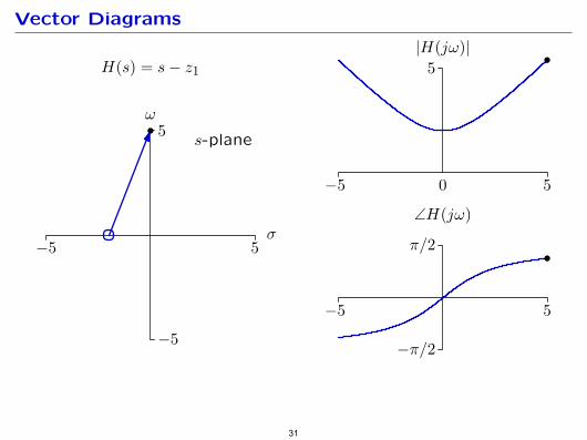
31

s-plane

σ

ω5

−5

5−5

H(s) = s− z1

−5 0 5

5|H(jω)|

−5 5

π/2

−π/2

∠H(jω)

Vector Diagrams

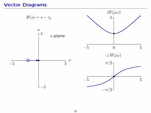
32

Vector Diagrams

s-plane

σ

ω5

−5

5−5

H(s) = s− z1

−5 0 5

5|H(jω)|

−5 5

π/2

−π/2

∠H(jω)

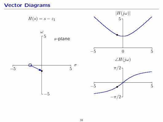
33

Vector Diagrams

s-plane

σ

ω5

−5

5−5

H(s) = s− z1

−5 0 5

5|H(jω)|

−5 5

π/2

−π/2

∠H(jω)

34

Vector Diagrams

s-plane

σ

ω5

−5

5−5

H(s) = s− z1

−5 0 5

5|H(jω)|

−5 5

π/2

−π/2

∠H(jω)

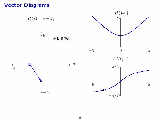
35

Vector Diagrams

s-plane

σ

ω5

−5

5−5

H(s) = s− z1

−5 0 5

5|H(jω)|

−5 5

π/2

−π/2

∠H(jω)

36

s-plane

σ

ω5

−5

5−5

H(s) = s− z1

−5 0 5

5|H(jω)|

−5 5

π/2

−π/2

∠H(jω)

Vector Diagrams

37

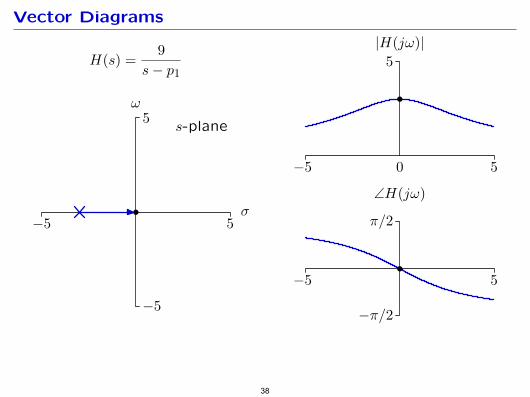
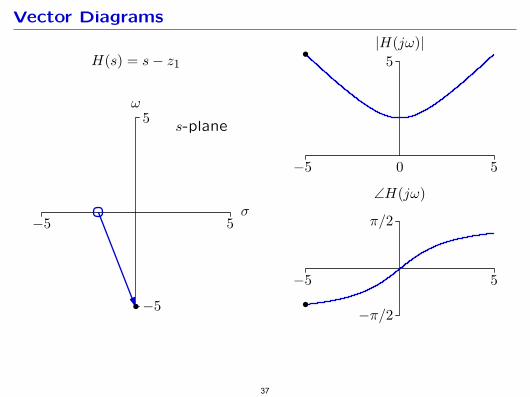
Vector Diagrams

s-plane

σ

ω5

−5

5−5

H(s) = 9s− p1

−5 0 5

5|H(jω)|

−5 5

π/2

−π/2

∠H(jω)

38

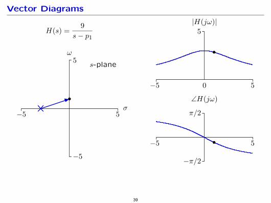
Vector Diagrams

s-plane

σ

ω5

−5

5−5

H(s) = 9s− p1

−5 0 5

5|H(jω)|

−5 5

π/2

−π/2

∠H(jω)

39

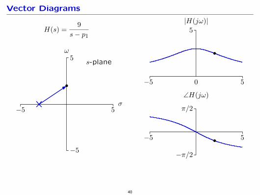
Vector Diagrams

s-plane

σ

ω5

−5

5−5

H(s) = 9s− p1

−5 0 5

5|H(jω)|

−5 5

π/2

−π/2

∠H(jω)

40

Vector Diagrams

s-plane

σ

ω5

−5

5−5

H(s) = 9s− p1

−5 0 5

5|H(jω)|

−5 5

π/2

−π/2

∠H(jω)

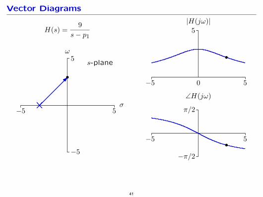
41

s-plane

σ

ω5

−5

5−5

H(s) = 9s− p1

−5 0 5

5|H(jω)|

−5 5

π/2

−π/2

∠H(jω)

Vector Diagrams

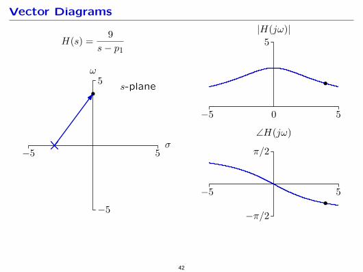
42

Vector Diagrams

s-plane

σ

ω5

−5

5−5

H(s) = 9s− p1

−5 0 5

5|H(jω)|

−5 5

π/2

−π/2

∠H(jω)

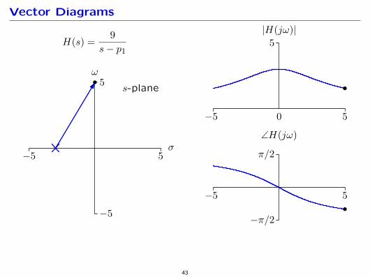
43

Vector Diagrams

s-plane

σ

ω5

−5

5−5

H(s) = 3 s− z1s− p1

−5 0 5

5|H(jω)|

−5 5

π/2

−π/2

∠H(jω)

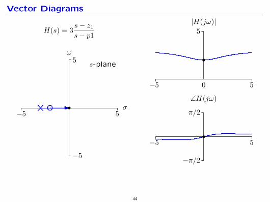
44

Vector Diagrams

s-plane

σ

ω5

−5

5−5

H(s) = 3 s− z1s− p1

−5 0 5

5|H(jω)|

−5 5

π/2

−π/2

∠H(jω)

45

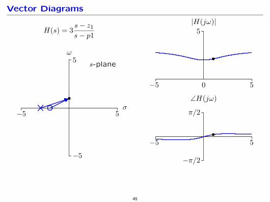
Vector Diagrams

s-plane

σ

ω5

−5

5−5

H(s) = 3 s− z1s− p1

−5 0 5

5|H(jω)|

−5 5

π/2

−π/2

∠H(jω)

46

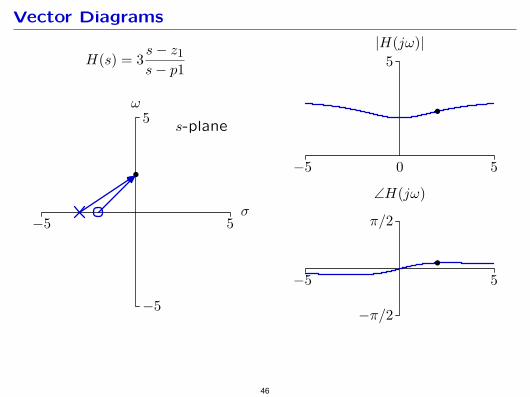
s-plane

σ

ω5

−5

5−5

H(s) = 3 s− z1s− p1

−5 0 5

5|H(jω)|

−5 5

π/2

−π/2

∠H(jω)

Vector Diagrams

47

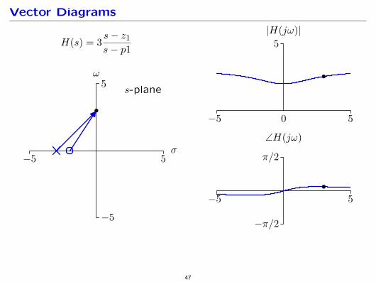
Vector Diagrams

s-plane

σ

ω5

−5

5−5

H(s) = 3 s− z1s− p1

−5 0 5

5|H(jω)|

−5 5

π/2

−π/2

∠H(jω)

48

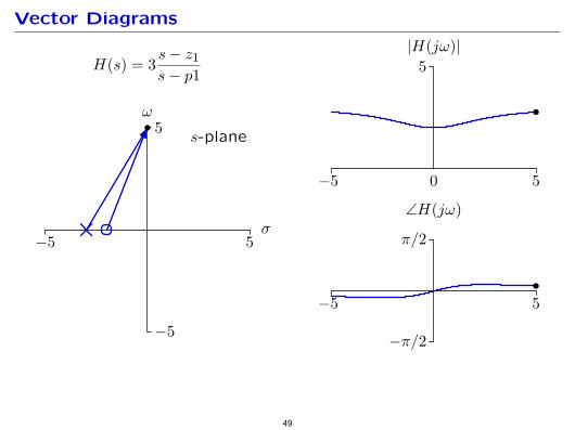
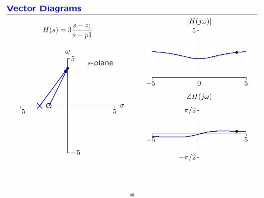
Vector Diagrams

s-plane

σ

ω5

−5

5−5

H(s) = 3 s− z1s− p1

−5 0 5

5|H(jω)|

−5 5

π/2

−π/2

∠H(jω)

49

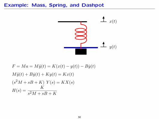
Example: Mass, Spring, and Dashpot

x(t)

y(t)

F = Ma = M y(t) = K(x(t) − y(t)) − By(t)

My(t) + By(t) + Ky(t) = Kx(t)

(s 2M + sB + K) Y (s) = KX(s) K

H(s) = s2M + sB + K

50

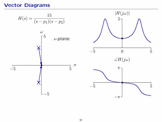
Vector Diagrams

s-plane

σ

ω5

−5

5−5

H(s) = 15(s− p1)(s− p2)

−5 0 5

5|H(jω)|

−5 5

π

−π

∠H(jω)

51

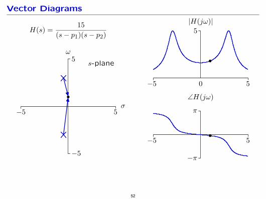
s-plane

σ

ω5

−5

5−5

H(s) = 15(s− p1)(s− p2)

−5 0 5

5|H(jω)|

−5 5

π

−π

∠H(jω)

Vector Diagrams

52

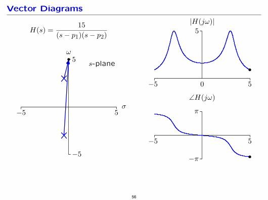
Vector Diagrams

s-plane

σ

ω5

−5

5−5

H(s) = 15(s− p1)(s− p2)

−5 0 5

5|H(jω)|

−5 5

π

−π

∠H(jω)

53

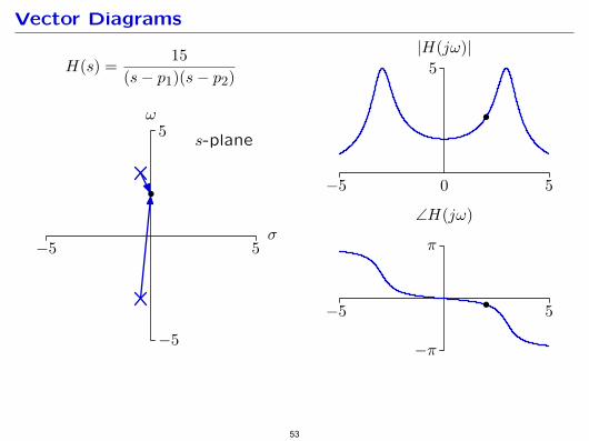
Vector Diagrams

s-plane

σ

ω5

−5

5−5

H(s) = 15(s− p1)(s− p2)

−5 0 5

5|H(jω)|

−5 5

π

−π

∠H(jω)

54

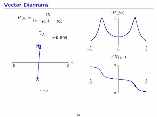
Vector Diagrams

s-plane

σ

ω5

−5

5−5

H(s) = 15(s− p1)(s− p2)

−5 0 5

5|H(jω)|

−5 5

π

−π

∠H(jω)

55

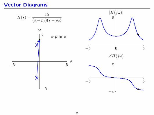
Vector Diagrams

s-plane

σ

ω5

−5

5−5

H(s) = 15(s− p1)(s− p2)

−5 0 5

5|H(jω)|

−5 5

π

−π

∠H(jω)

56

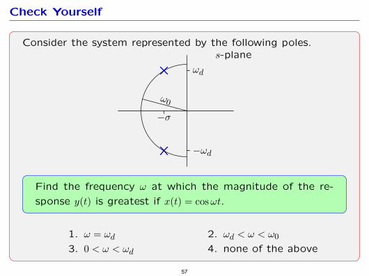
Check Yourself

Consider the system represented by the following poles.

ω0

s-plane

−σ

ωd

−ωd

Find the frequency ω at which the magnitude of the re­

sponse y(t) is greatest if x(t) = cos ωt.

1. ω = ωd 2. ωd < ω < ω0

3. 0 < ω < ωd 4. none of the above

57

� �� �

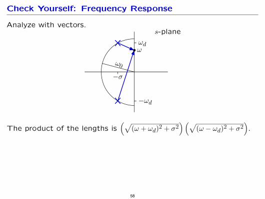
Check Yourself: Frequency Response

Analyze with vectors.

ω0

s-plane

−σ

ωd

−ωd

ω

The product of the lengths is (ω + ωd)2 + σ2 (ω − ωd)2 + σ2 . � �

58

( )( )

�� ��� �

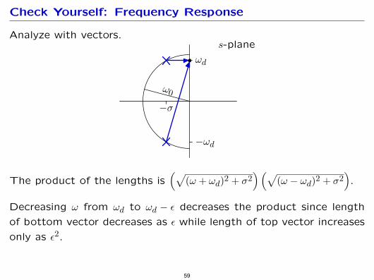
Check Yourself: Frequency Response

Analyze with vectors.

ω0

s-plane

−σ

ωd

−ωd

The product of the lengths is (ω − ωd)2 + σ2 .(ω + ωd)2 + σ2

Decreasing ω from ωd to ωd − E decreases the product since length

of bottom vector decreases as E while length of top vector increases

only as E2 .

59

(√ )(√ )

�� ��� �� �� �

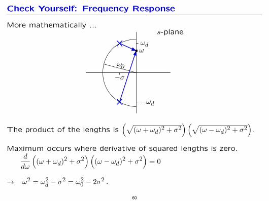
Check Yourself: Frequency Response

More mathematically ...

ω0

s-plane

−σ

ωd

−ωd

ω

The product of the lengths is (ω + ωd)2 + σ2 (ω − ωd)2 + σ2 .

Maximum occurs where derivative of squared lengths is zero. d (ω + ωd)2 + σ2 (ω − ωd)2 + σ2 = 0

dω

→ ω2 = ω2 − σ2 = ω02 − 2σ2 .d

60

(√ )(√ )( )( )

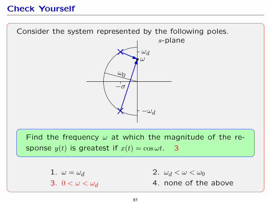
Check Yourself

Consider the system represented by the following poles.

ω0

s-plane

−σ

ωd

−ωd

ω

Find the frequency ω at which the magnitude of the re­

sponse y(t) is greatest if x(t) = cos ωt. 3

1. ω = ωd 2. ωd < ω < ω0

3. 0 < ω < ωd 4. none of the above

61

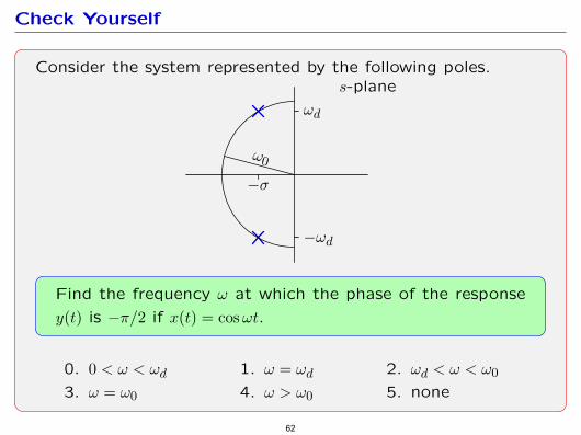
Check Yourself

Consider the system represented by the following poles.

ω0

s-plane

−σ

ωd

−ωd

Find the frequency ω at which the phase of the response

y(t) is −π/2 if x(t) = cos ωt.

0. 0 < ω < ωd 1. ω = ωd 2. ωd < ω < ω0

3. ω = ω0 4. ω > ω0 5. none

62

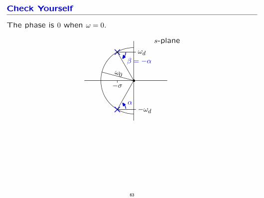
Check Yourself

The phase is 0 when ω = 0.

ω0

s-plane

−σ

ωd

−ωdα

β = −α

63

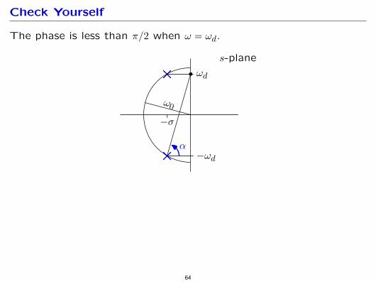
Check Yourself

The phase is less than π/2 when ω = ωd.

ω0

s-plane

−σ

ωd

−ωdα

64

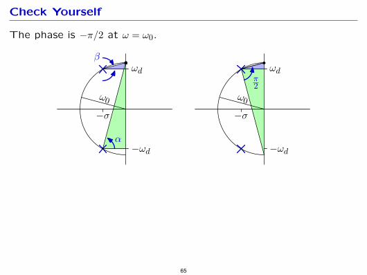
Check Yourself

The phase is −π/2 at ω = ω0.

ω0

−σ

ωd

−ωdα

β

ω0

−σ

ωd

−ωd

π2

65

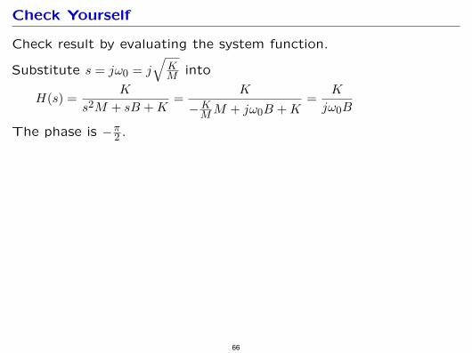
Check Yourself

Check result by evaluating the system function. Substitute s = jω0 = j K

M into

K K K = =H(s) = 2M + sB + K −K M M + jω0B + K jω0Bs

The phase is −π 2 .

66

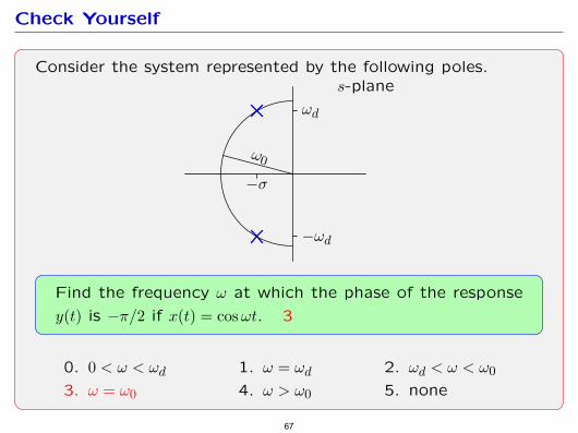
Check Yourself

Consider the system represented by the following poles.

ω0

s-plane

−σ

ωd

−ωd

Find the frequency ω at which the phase of the response

y(t) is −π/2 if x(t) = cos ωt. 3

0. 0 < ω < ωd 1. ω = ωd 2. ωd < ω < ω0

3. ω = ω0 4. ω > ω0 5. none

67

Frequency Response: Summary

LTI systems can be characterized by responses to eternal sinusoids.

Many systems are naturally described by their frequency response.

– audio systems

– mass, spring, dashpot system

Frequency response is easy to calculate from the system function.

Frequency response lives on the jω axis of the Laplace transform.

68

MIT OpenCourseWarehttp://ocw.mit.edu

6.003 Signals and SystemsFall 2011

For information about citing these materials or our Terms of Use, visit: http://ocw.mit.edu/terms.