Lecture 8 Instrumental Variables - Bauer College of Business · PDF fileRS – Lecture 8 1...

RS – Lecture 8

1

1

Lecture 8Instrumental Variables

• Last lecture, we presented a new set of assumptions for the CLM:

(A1) DGP: y = X + . (A2’) X stochastic, but E[X’ ]= 0 and E[ε]=0.

(A3) Var[|X] = σ2 IT

(A4’) plim (X’X/T) = Q (p.d. matrix with finite elements, rank= k)

• We studied the large sample properties of OLS:

- b and s2 are consistent

- b N(β, (σ2/T) Q-1)

- t-tests asymptotically N(0,1), Wald tests asymptotically 2rank(ST) and

F-tests asymptotically 2rank(Var[m]) .

- Small sample behavior may be understood by simulations and/or bootstrapping.

CLM: New Assumptions

a

RS – Lecture 8

2

• We start with our CLM:y = X + . (DGP)

- Let's pre-multiplying the DGP by X'X' y = X' X + X' .

- We can interpret b as the solution obtained by first approximating X' by zero, and then solving the k equations in k unknowns

X'y = X'X b (normal equations).

Note: What makes b consistent when X'/T 0 is that approximating (X'/T ) by 0 is reasonably accurate in large samples.

• Now, we challenge this approximation. We relax the assumption that {xi,εi} is a sequence of independent observations. That is,

plim (X’/T) ≠ 0. => This is the IV Problem!

p

The IV Problem

• A correlation between X & is not rare in economics, especially in corporate finance, where endogeneity is pervasive.

• Endogenous in econometrics: A variable is correlated with the error term.

• Q: What is the implication of the violation of plim(X’/T) = 0?

From the asymptotic CLM version, we keep (A1), (A3), and (A4’):(A1) y = X + .(A3) Var[|X] = σ2 IT

(A4’) plim (X’X/T) = Q

• Now, we assume (A2’’) plim(X’/T) ≠ 0.

• Then, plim b = plim + plim (X’X/T)-1 plim (X/T)

The IV Problem: OLS is Inconsistent

RS – Lecture 8

3

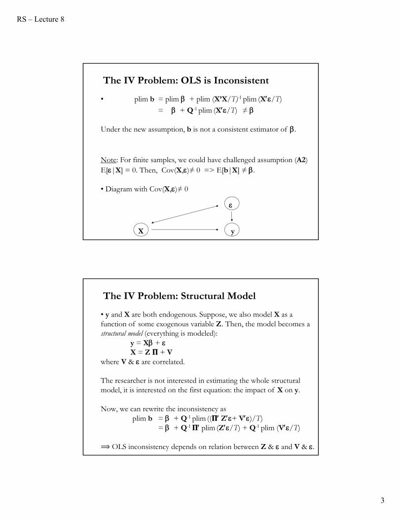
• plim b = plim + plim (X’X/T)-1 plim (X/T)

= + Q-1 plim (X/T) ≠

Under the new assumption, b is not a consistent estimator of .

Note: For finite samples, we could have challenged assumption (A2)E[|X] = 0. Then, Cov(X,)≠ 0 => E[b|X] ≠ .

• Diagram with Cov(X,)≠ 0

The IV Problem: OLS is Inconsistent

X y

• y and X are both endogenous. Suppose, we also model X as a function of some exogenous variable Z. Then, the model becomes a structural model (everything is modeled):

y = X + X = Z + V

where V & are correlated.

The researcher is not interested in estimating the whole structural model, it is interested on the first equation: the impact of X on y.

Now, we can rewrite the inconsistency asplim b = + Q-1 plim (( Z+ V)/T)

= + Q-1 plim (Z/T) + Q-1 plim (V/T)

⟹ OLS inconsistency depends on relation between Z & and V & .

The IV Problem: Structural Model

RS – Lecture 8

4

• Suppose we want to study the relation between a firm’s CEO’s compensation (y) and a CEO’s network (x).

Usually, a linear regression model is used, relating y and x, with additional “control variables” (W) controlling for other features that make one CEO’s compensation different from another. The term represents the effects of individual variation that have not been controlled for with W or x.

The model is: y = x + Wγ +

If a CEO’s network is influenced by the CEO’s natural skills, we have a problem: y and x are both endogenous –i.e., influenced by the unobserved CEO’s skills, say S.

The IV Problem: Example 1

• y and x are both influenced by an unobservable variable. Then, Cov(x, )≠0 (=> by LLN, plim (X’/T) ≠ 0)

• It looks like an omitted variable problem. Assuming linearity, it can be solved by adding as a control variable “CEO’s skills,” S:

y = x + Wγ + S +

However, S is unobservable.

Note: x is endogenous. It needs a model! Say, it depends on Z:

x = Z π + v (where σεV measures the endogeneity of x.)

• Recall: Endogeneity occurs when a variable, X, is correlated with .


RS – Lecture 8

5

• Suppose we want to study the effect of military service (x) on earnings (y). We use a linear model, adding some control variables (W), controlling for other features that affect y:

y = x + Wγ +

would measure “the causal effect” we would get if x were randomly assigned. But, there is selection bias by both individuals and military recruiters.

That is, x is not randomly assigned: Unobserved factors that affect y, also affect x ⟹ Cov(x,) ≠ 0. .


• In this example, we introduce measurement error in X. That is, DGP:y = x* + ~ iid D(0, σε2)

x = x* + u u ~ iid D(0, σu2) -no correlation to

We are interested in x*, and its marginal effect , but we observe/measure x, which measures x* with error (u).

All of the CLM assumptions apply. Then,

y = (x-u) + = x + - u = x + w

E[x’w] = E[(x*+u)’(-u)] = -σu2 ≠ 0 & plim (X’w/T)≠0

⟹ CLM assumptions violated => OLS inconsistent!


RS – Lecture 8

6

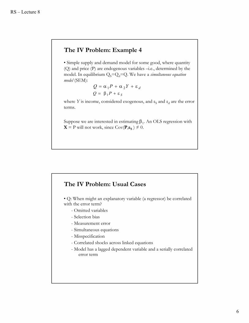
• Simple supply and demand model for some good, where quantity (Q) and price (P) are endogenous variables –i.e., determined by the model. In equilibrium QS=Qd=Q. We have a simultaneous equation model (SEM):

where Y is income, considered exogenous, and εS and εd are the error terms.

Suppose we are interested in estimating 1. An OLS regression with X = P will not work, since Cov(P,εS ) ≠ 0.


SPQ 1

dYPQ 21

• Q: When might an explanatory variable (a regressor) be correlated with the error term?

- Omitted variables- Selection bias- Measurement error- Simultaneous equations - Misspecification- Correlated shocks across linked equations- Model has a lagged dependent variable and a serially correlated

error term

The IV Problem: Usual Cases

RS – Lecture 8

7

Instrumental Variables: New CLM Assumptions

• New Framework: (A1) DGP: y = X + . (A2’’) plim (X’/T) ≠ 0 (A3) Var[|X] = σ2 IT

(A4’) plim (X’X/T) = Q (p.d. matrix, with rank k)⇒ b is not a consistent estimator of .

• Q: How can we construct a consistent estimator of ?We will assume that there exists a set of l variables, Z such that

(1) plim (Z’X/T) 0 (relevant condition)(2) plim (Z’/T) = 0 (valid condition)

• The variables in Z are called instrumental variables (IVs). In general, not all the X will be correlated with error .

• We can also write the new framework, emphasizing endogeneity, as: (A1) DGP: y = Y + U γ + . (A2’’) plim (Y’ /T) ≠ 0 (Y: “problem,” endogenous, variables)(A2’’) plim (U’ /T) = 0 (U: clean variables)(A3) Var[|Y,U] = σ2 IT

(A4) Y and U have full column rank. Say kx and ku.

• We have Z, a matrix of l “excluded instruments” –the IVs. The IVs have no impact on y except through Y. We relate Y to Z linearly by:

Y = Z П + U Φ + V - V ~ D(0, σV2 IT)

Note: When the number kx of “endogenous” variables is greater than one, we have a system of multiple equations. The estimation of this equation is called “first stage.”

Instrumental Variables: Endogeneity

RS – Lecture 8

8

• Concentrating on two equations (and let X=Y): (A1) y = X + U γ + (called structural equation)

X = Z П + U Φ + V (first stage regression)

Replacing the second equation in (A1):y = (Z П + U Φ + V) + U γ + = Z П + U φ + ξ

This equation is called reduced form, where φ = Φ + γξ = V +

Note: Usually, V and are N(0, σJJ I). But, they can be correlated.

• In this lecture, the parameter of interest is . OLS cannot estimate it. But OLS works on the reduced form to consistently estimate Г=П.

Instrumental Variables: Endogeneity

• Model:y = X + U γ + - structural equationX = Z П + U Φ + V - first stage equationy = + U γ + - second stage equationy = Z Г + U φ + ξ - reduced form

• Variablesy, X: endogenous variables –i.e., correlated with .U & Z: exogenous variables –i.e., uncorrelated with .U: included instruments, clean variables (“controls”)Z: excluded instruments, IVs –i.e., satisfies the relevant condition and the valid condition, also referred as exclusion restriction. (Excluded = not included in the structural equation.)

Instrumental Variables: Notation

RS – Lecture 8

9

• Parameters: Structural parameter, usually the parameter of interestП: 1st-stage parameter. It captures the strength of the IV, Z.

If П≈0, not very powerful. Г: Reduced form parameter. It can show the potential of Z as

instrument.

• EquationsStructural equation: Theory dictates this relation: it relates y and X(or Y). It measures the causal effect of X on y, ; but the effect is blurred by endogeneity. First stage: Regression of X on the instrument, Z (it measures a causal effect from Z to X).

Reduced form: Regression of y earnings on the instrument is called the reduced form (it measures the direct causal effect from Z to y).

Instrumental Variables: Notation

• New assumption: we have l IVs, Z, such that

plim(Z’X/T) 0 but plim(Z’/T) = 0

• Then, we state assumptions to construct an alternative (to OLS) consistent estimator of .

Assumptions:

{xi, zi, εi} is a sequence of RVs, with:

E[X’X] = Qxx (pd and finite) (LLN => plim(X’X/T) =Qxx )

E[Z’Z] = Qzz (finite) (LLN => plim(Z’Z/T) =Qzz )

E[Z’X] = Qzx (pd and finite) (LLN => plim(Z’X/T) =Qzx )

E[Z’] = 0 (LLN => plim(Z’/T) = 0)

Instrumental Variables: Assumptions

RS – Lecture 8

10

• To construct a new estimator, we start by pre-multiplying the DGP by W'Z’, where W l×k weighting matrix that we choose:

W'Z’y = W'Z’(X+) = W'Z’X+ W'Z’⇒ W helps to create a k ×k square matrix, needed for inversion.

• Following the same idea as in OLS, we get a system of equations: W'Z’X bIV = W'Z’y

• We have two cases where estimation is possible:- Case 1: l = k -i.e., number of instruments = number of regressors.- Case 2: l > k -i.e., number of instruments > number of regressors.

The second case is the usual situation. We can throw l-k instruments, but throwing away information is never optimal.

Instrumental Variables: Estimation

• Case 1: l = k -i.e., number of instruments = number of regressors.

To get the IV estimator, we start from the system of equations: W'Z’X bIV = W'Z’y

- dim(Z)=dim(X): Txk ⇒ Z’X is a kxk pd matrix

- In this case, W is irrelevant, say, W=I. Then,

bIV = (Z’X)-1Z’y

Note: Let Z = X. Then,

bIV = b = (X’X)-1Xy

IV Estimation

That is, under the usual assumptions, b is an IV estimator with X as its own instrument.

Sewall G. Wright (1889 – 1988, USA)

RS – Lecture 8

11

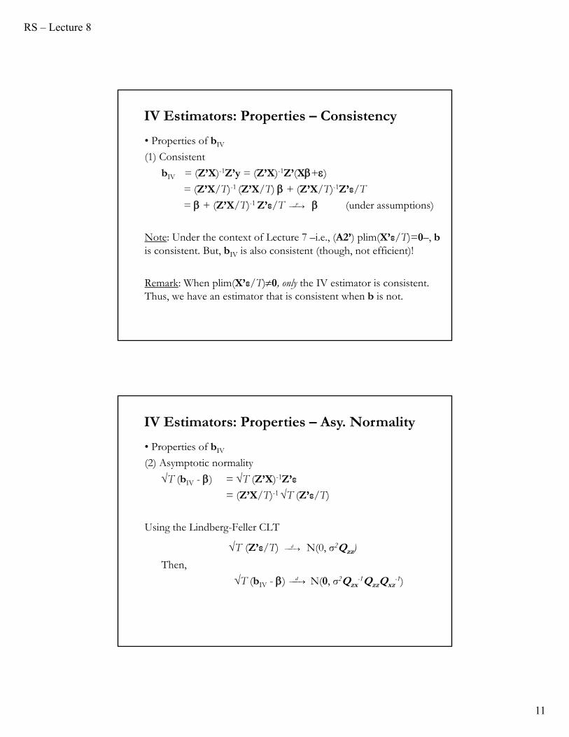
• Properties of bIV

(1) Consistent

bIV = (Z’X)-1Z’y = (Z’X)-1Z’(X+)= (Z’X/T)-1 (Z’X/T) + (Z’X/T)-1Z’ε/T

= + (Z’X/T)-1 Z’ε/T (under assumptions)

Note: Under the context of Lecture 7 –i.e., (A2’) plim(X’ε/T)=0–, bis consistent. But, bIV is also consistent (though, not efficient)!

Remark: When plim(X’ε/T)0, only the IV estimator is consistent. Thus, we have an estimator that is consistent when b is not.

p

IV Estimators: Properties – Consistency

• Properties of bIV

(2) Asymptotic normality

T (bIV - ) = T (Z’X)-1Z’ε

= (Z’X/T)-1 T (Z’ε/T)

Using the Lindberg-Feller CLT

T (Z’ε/T) N(0, σ2Qzz)

Then,

T (bIV - ) N(0, σ2Qzx-1QzzQxz

-1)

d

d

IV Estimators: Properties – Asy. Normality

RS – Lecture 8

12

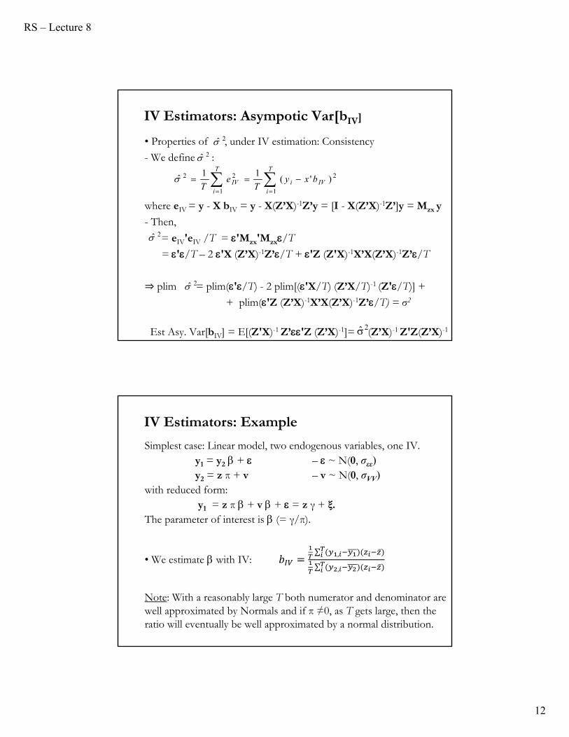
• Properties of , under IV estimation: Consistency

- We define :

where eIV = y - X bIV = y - X(Z’X)-1Z’y = [I - X(Z’X)-1Z’]y = Mzx y

- Then,

= eIV'eIV /T = 'Mzx'Mzx/T

= '/T – 2 'X (Z’X)-1Z’/T + 'Z (Z'X)-1X’X(Z’X)-1Z’/T

⇒ plim = plim('/T) - 2 plim[('X/T) (Z’X/T)-1 (Z'/T)] +

+ plim('Z (Z’X)-1X’X(Z’X)-1Z’/T) = σ2

Est Asy. Var[bIV] = E[(Z'X)-1 Z’'Z (Z’X)-1]= (Z’X)-1 Z'Z(Z’X)-1

2

11

22 )'(11

ˆ IV

T

ii

T

iIV bxy

Te

T

2̂2̂

2̂

2̂

2̂

IV Estimators: Asympotic Var[bIV]

Simplest case: Linear model, two endogenous variables, one IV. y1 = y2 + – ~ N(0, σεε)y2 = z π + v – v ~ N(0, σVV)

with reduced form:y1 = z π + v + = z γ + ξ.

The parameter of interest is (= γ/π).

• We estimate with IV:∑ , ̅

∑ , ̅

Note: With a reasonably large T both numerator and denominator are well approximated by Normals and if π ≠0, as T gets large, then the ratio will eventually be well approximated by a normal distribution.

IV Estimators: Example

RS – Lecture 8

13

• To analyze the bias, bIV = (z' y2)-1 z' y1 = + (z' y2)-1 z'

plim(bIV) - = plim(z’/T)/plim(z’y2/T) Cov(z,)/Cov(z,y2)

• When Cov(z,) ≠ 0, IV estimation is inconsistent.

• If Cov(z,) is small, but π≈0, the inconsistency can get large (π≈0)

⇒ Cov(z,y2) = Cov(z,(zπ+v)) = π Var(z) + Cov(z,v) = π Var(z) ≈ 0

• When π=0, Cov(z,y2)=0, the IV estimator is not defined. When π=0, the instrument provides no information. It is an irrelevant instrument.


p

• When π is small, we say z is a weak instrument. It provides information, but, as we will see later, not enough.

• Note that even when π=0, in finite samples, the sample analogue to Cov(z,y2)≠0. Not very useful fact, the sampling variation in Cov(z,y2) is not helpful to estimate .

Note: The weak instrument literature is concerned with testing H0:=0 when π is too close to 0. As we will see later, the normal approximation to the ratio will not be accurate.


RS – Lecture 8

14

• We assume that there exists a set of l variables, Z such that (1) plim (Z’X/T) 0 (relevant condition)(2) plim (Z’/T) = 0 (valid condition –or exclusion restriction)

• We are going to use the variation in Z, which is uncorrelated with , to explain the variation of y. Condition (1) allows to do this. Suppose the relation between Z, X and y is given in the following diagram:

X Y

Z

Now, not all the variation in X is used. Only the portion of Xwhich is “explained” by Z can be used to explain y.

IV Estimators: Weak and Strong Instruments

• Best situation : A lot of X is explained by Z, and most of the overlap between X and Y is accounted for.⇒ Z is a strong IV.

Usual situation : Not a lof of X is explained by Z, or what is explained does not overlap much with Y.

⇒ Z is a weak IV.

X Y

Z

X Y

Z

IV Estimators: Weak and Strong Instruments

RS – Lecture 8

15

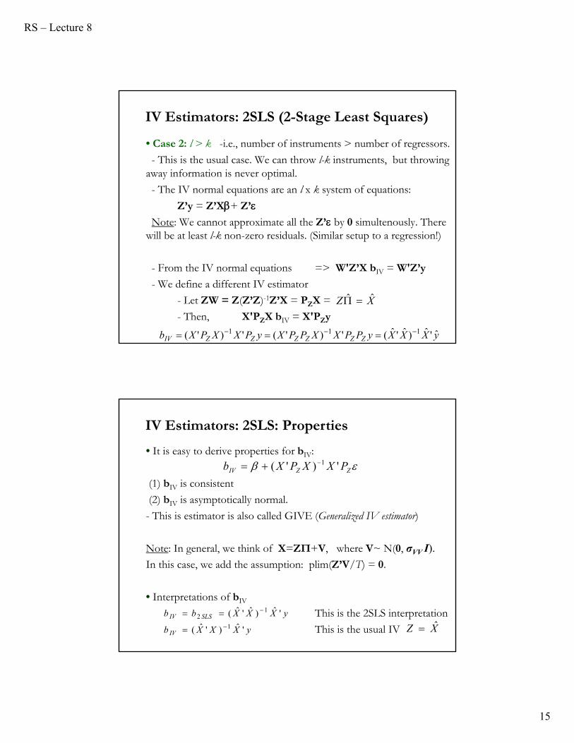
• Case 2: l > k -i.e., number of instruments > number of regressors.

- This is the usual case. We can throw l-k instruments, but throwing away information is never optimal.

- The IV normal equations are an l x k system of equations:

Z’y = Z’X+ Z’Note: We cannot approximate all the Z’ by 0 simultenously. There

will be at least l-k non-zero residuals. (Similar setup to a regression!)

- From the IV normal equations => W'Z’X bIV = W'Z’y

- We define a different IV estimator

- Let ZW = Z(Z’Z)-1Z’X = PZX =

- Then, X'PZX bIV = X'PZy

yXXXyPPXXPPXyPXXPXb ZZZZZZIV ˆ'ˆ)ˆ'ˆ(')'(')'( 111

IV Estimators: 2SLS (2-Stage Least Squares)

XZ ˆˆ

• It is easy to derive properties for bIV:

(1) bIV is consistent

(2) bIV is asymptotically normal.

- This is estimator is also called GIVE (Generalized IV estimator)

Note: In general, we think of X=ZП+V, where V~ N(0, σVV I).

In this case, we add the assumption: plim(Z’V/T) = 0.

• Interpretations of bIV

This is the 2SLS interpretation

This is the usual IV XZ ˆyXXXb

yXXXbb

IV

SLSIV

'ˆ)'ˆ(

'ˆ)ˆ'ˆ(1

12

IV Estimators: 2SLS: Properties

ZZIV PXXPXb ')'( 1

RS – Lecture 8

16

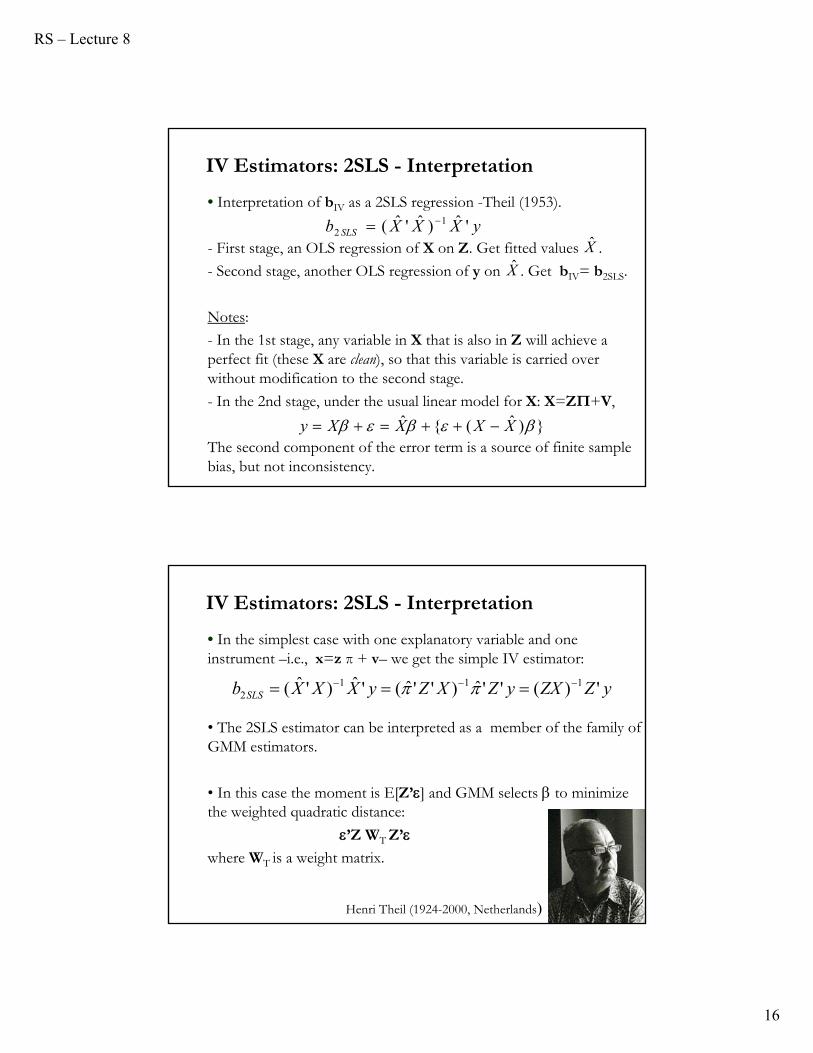
• Interpretation of bIV as a 2SLS regression -Theil (1953).

- First stage, an OLS regression of X on Z. Get fitted values .

- Second stage, another OLS regression of y on . Get bIV= b2SLS.

Notes:

- In the 1st stage, any variable in X that is also in Z will achieve a perfect fit (these X are clean), so that this variable is carried over without modification to the second stage.

- In the 2nd stage, under the usual linear model for X: X=ZП+V,

The second component of the error term is a source of finite sample bias, but not inconsistency.

X̂

yXXXb SLS 'ˆ)ˆ'ˆ( 12

X̂

IV Estimators: 2SLS - Interpretation

})ˆ({ˆ XXXXy

• In the simplest case with one explanatory variable and one instrument –i.e., x=z π + v– we get the simple IV estimator:

• The 2SLS estimator can be interpreted as a member of the family of GMM estimators.

• In this case the moment is E[Z’] and GMM selects to minimize the weighted quadratic distance:

’Z WT Z’where WT is a weight matrix.

yZZXyZXZyXXXb SLS ')(''ˆ)''ˆ('ˆ)'ˆ( 1112

Henri Theil (1924-2000, Netherlands)

IV Estimators: 2SLS - Interpretation

RS – Lecture 8

17

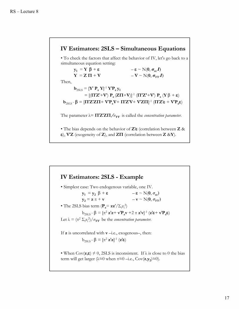
• To check the factors that affect the behavior of IV, let's go back to a simultaneous equation setting:

y1 = Y + – ~ N(0, σεε I)Y = Z П + V – V ~ N(0, σVV I)

Then,

b2SLS = [Y' Pz Y]-1 Y'Pz y1

= [(П'Z'+V') Pz (ZП+V)]-1 (П'Z'+V') Pz (Y + )b2SLS - = [П'Z'ZП+ V'PzV+ П'Z'V+ V'ZП]-1 (П'Z' + V'Pz)

The parameter λ= П'Z'ZП/σVV is called the concentration parameter.

• The bias depends on the behavior of Z' (correlation between Z &), V'Z (exogeneity of Z), and ZП (correlation between Z &Y).

IV Estimators: 2SLS – Simultaneous Equations

• Simplest case: Two endogenous variable, one IV. y1 = y2 + – ~ N(0, σεε)y2 = z π + v – v ~ N(0, σVV)

• The 2SLS bias term (Pz= zz'/Σizi2)

b2SLS - = [π2 z'z+ v'Pzv +2 π z'v]-1 (z'+ v'Pz) Let λ = (π2 Σizi

2)/σVV be the concentration parameter.

If z is uncorrelated with v –i.e., exogenous–, then:

b2SLS - = [π2 z'z]-1 (z')

• When Cov(z,) ≠ 0, 2SLS is inconsistent. If λ is close to 0 the bias term will get larger (λ≈0 when π≈0 –i.e., Cov(z,y2)≈0).

IV Estimators: 2SLS - Example

RS – Lecture 8

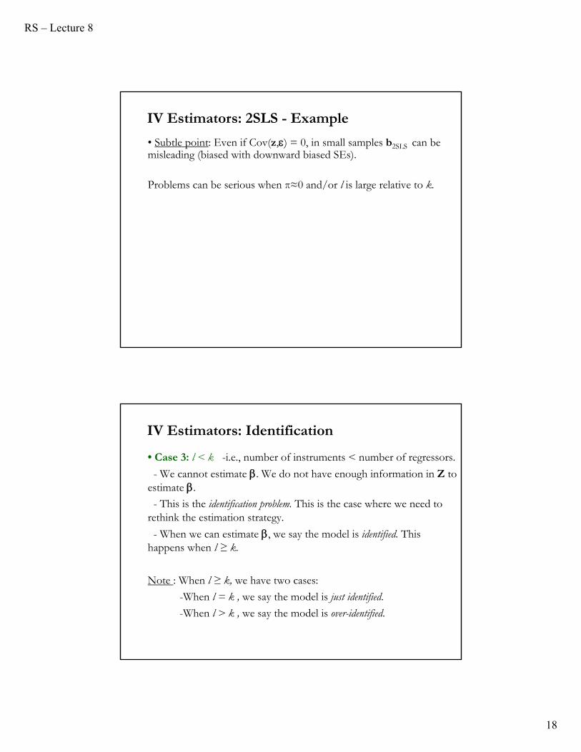
18

• Subtle point: Even if Cov(z,) = 0, in small samples b2SLS can be misleading (biased with downward biased SEs).

Problems can be serious when π≈0 and/or l is large relative to k.

IV Estimators: 2SLS - Example

• Case 3: l < k -i.e., number of instruments < number of regressors.

- We cannot estimate . We do not have enough information in Z to estimate .

- This is the identification problem. This is the case where we need to rethink the estimation strategy.

- When we can estimate , we say the model is identified. This happens when l ≥ k.

Note : When l ≥ k, we have two cases:

-When l = k , we say the model is just identified.

-When l > k , we say the model is over-identified.

IV Estimators: Identification

RS – Lecture 8

19

Asymptotic Covariance Matrix for 2SLS (Greene)

12

11222

112

)ˆ'ˆ(

)'ˆ')(ˆ'ˆ()'ˆ(])')([(

)')('()'(])')([(

XX

XXXXXXbbE

ZXZZXZbbE

SLSSLS

IVIV

• The asymptotic variance for the IV and 2SLS is given by:

221

2 )(1

ˆ SLSi

T

i i bxyT

• To estimate Asy Var[b2SLS] we need to estimate σε2:

• Do not use the inconsistent estimator:

221

2 )ˆ(1

ˆ SLSi

T

i i bxyT


]ˆ][[(

)')(']()')('][([(

)')('()')('()'(

)')('()'(][(

11

11

1112

112

OLS

OLS

IV

bV

ZXZZXZXXbV

ZXZZXZXXXX

ZXZZXZbV

• A little bit of algebra relates the asymptotic variances of bIV & bOLS:

where we assume X=ZП+V and Φ is the coefficient in the reverse first stage regression.

Two things to notice:

- As Z ⟶X, V[bIV] ⟶ V[bOLS].

- As Cov(Z,X) gets smaller –i.e., Z becomes a weak instrument-, V[bIV]gets larger.

RS – Lecture 8

20


⇒ Weak instruments create big uncertainty about b2SLS.

12

122

)ˆ''ˆ(

)ˆ'ˆ(][(

ZZ

XXbV SLS

• This relation between Cov(Z,X) and estimation uncertainty also applies to the 2SLS estimators:

2 -1

2 -1

A comparison to OLSˆ ˆAsy.Var[2SLS]= ( ' )

Neglecting the inconsistency,

Asy.Var[LS] = ( ' )(This is the variance of LS around its mean, not )Asy.Var[2SLS] Asy.Var[LS] in the matrix sense.Com

X X

X Xβ

-1 -1 2

2 2Z Z

pare inverses:ˆ ˆ{Asy.Var[LS]} - {Asy.Var[2SLS]} (1 / )[ ' ' ]

(1 / )[ ' '( ) ]=(1 / )[ ' ]

This matrix is nonnegative definite. (Not positive definiteas it m ight have some rows and columns

X X - X X

X X - X I M X X M X

which are zero.)Implication for "precision" of 2SLS.The problem of "Weak Instruments"

2SLS Has Larger Variance than OLS (Greene)

RS – Lecture 8

21

• The variance is larger than that of OLS. (A large sample type of Gauss-Markov result is at work.)(1) OLS is inconsistent.(2) Mean squared error is uncertain:

MSE[estimator|] = Variance + square of bias.

For a long time, IV was thought to be “the cure” to the biases introduced by OLS. But, in terms of MSE, IV may be better or worse. It depends on the data: X, Z and ε.

Asymptotic Efficiency (Greene)

• A popular misconception. If only one variable in X is correlated with , the other coefficients are consistently estimated. False.

The problem is “smeared” over the other coefficients.

1

1 11

2 1-1

1

1

1

S u ppo se o n ly th e firs t va r ia b le is co rre la te d w ith

0U n de r th e a ssu m p tio n s , p lim ( /n ) = . T h en

....

0p lim = p lim ( /n )

... ....

t im e s

K

qq

q

ε

X 'ε

b - β X 'X

-1 th e firs t co lu m n o f Q

A Popular Misconception (Greene)

RS – Lecture 8

22

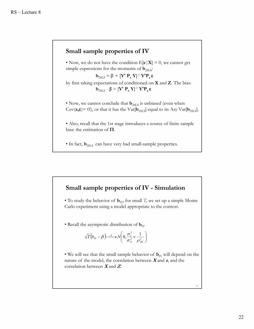
• Now, we do not have the condition E[ε|X] = 0, we cannot get simple expressions for the moments of b2SLS:

b2SLS = + [Y' Pz Y]-1 Y'Pz by first taking expectations of conditioned on X and Z. The bias:

b2SLS - β = [Y' Pz Y]-1 Y'Pz

• Now, we cannot conclude that b2SLS is unbiased (even when Cov(z,)= 0!), or that it has the Var[b2SLS] equal to its Asy Var[b2SLS].

• Also, recall that the 1st stage introduces a source of finite sample bias: the estimation of П.

• In fact, b2SLS can have very bad small-sample properties.

Small sample properties of IV

16

• To study the behavior of bIV, for small T, we set up a simple Monte Carlo experiment using a model appropriate to the context.

• Recall the asymptotic distribution of bIV

• We will see that the small sample behavior of bIV will depend on the nature of the model, the correlation between X and ε, and the correlation between X and Z.

22

2 1,0

XZX

dIV NbT

Small sample properties of IV - Simulation

RS – Lecture 8

23

17

• We start with a simple linear model:

with observations on Z, U, and ε are drawn independently from a N(0,1). We think of Z and U as variables and of ε as the error term in the model. π and π2 are constants.

• By construction, X is not independent of ε. OLS is inconsistent and its standard errors and tests will be invalid.

• Z is correlated with X, but independent of ε. It serves as an instrument. (U is included to provide some variation in X, not connected with either Z or ε.)

XY 21

UZX 21


20

• To start the simulation, we set:

π = 0.5, and π = 2.0.

• That is,

)1,0(~510 NiidXY )1,0(~);1,0(~0250 NiidUNiidZU.Z.X

• It is easy to check that plim b2,OLS = 5.19 (=5+1/(.52+22+1)). Of course, plim b2,IV = 5.00. We draw n=25, 100 & 3,200. We do 1 million simulations.


Sample Size b2,OLS (SE[b2,OLS ]) b2,IV (SE[b2,IV]) MSEs

n = 25 5.190 (0.080) 4.998 (0.137) .055 - .019

n = 100 5.191 (0.040) 5.000 (0.054) .038 - .003

n = 3200 5.191 (0.007) 5.000 (0.009) .036 - .0001

RS – Lecture 8

24

21

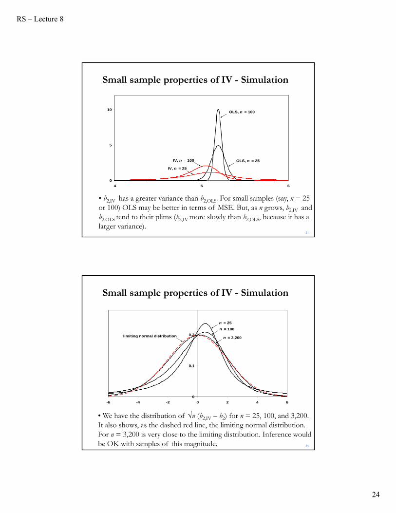
• b2,IV has a greater variance than b2,OLS. For small samples (say, n = 25 or 100) OLS may be better in terms of MSE. But, as n grows, b2,IV and b2,OLS tend to their plims (b2,IV more slowly than b2,OLS, because it has a larger variance).

0

5

10

4 5 6

OLS, n = 25

OLS, n = 100

IV, n = 100

IV, n = 25


24

• We have the distribution of √n (b2,IV – b2) for n = 25, 100, and 3,200. It also shows, as the dashed red line, the limiting normal distribution. For n = 3,200 is very close to the limiting distribution. Inference would be OK with samples of this magnitude.

0

0.1

0.2

-6 -4 -2 0 2 4 6

n = 25

n = 100

n = 3,200limiting normal distribution


RS – Lecture 8

25

24

• For n=25, 100, the tail are too fat. Inference would give rise to excess instances of Type I error (under rejection). The distortion for small sample sizes is partly attributable to the low ρxz corr(X,Z)=0.22 (=.5/sqrt(5.25)) (or weak instruments; common in IV estimation).

0

0.1

0.2

-6 -4 -2 0 2 4 6

n = 25

n = 100

n = 3,200limiting normal distribution


24

• To check the effect of ρxz on the estimation, we lower π to 0.01, which brings ρxz corr(X,Z)=0.0045 (=.1/sqrt(5.01)) and we increase π to 4, with ρxz 0.8729.


Empirical Type I Error

Sample Size ρ = .8729 ρ = .2182 ρ = .0045

n=25 0.0698 0.0717 0.0752

n = 100 0.0610 0.0628 0.0628

n = 3200 0.0511 0.0508 0.0527

• Some size problem for small n. Low ρxz slightly increases the size problem.

RS – Lecture 8

26

Cornwell and Rupert Data (Greene)

Cornwell and Rupert Returns to Schooling Data, 595 Individuals, 7 YearsVariables in the file are

EXP = work experienceWKS = weeks workedOCC = occupation, 1 if blue collar, IND = 1 if manufacturing industrySOUTH = 1 if resides in southSMSA = 1 if resides in a city (SMSA)MS = 1 if marriedFEM = 1 if femaleUNION = 1 if wage set by union contractED = years of educationBLK = 1 if individual is blackLWAGE = log of wage = dependent variable in regressions

These data were analyzed in Cornwell, C. and Rupert, P., "Efficient Estimation with Panel Data: An Empirical Comparison of Instrumental Variable Estimators," Journal of Applied Econometrics, 3, 1988, pp. 149-155. See Baltagi, page 122 for further analysis. The data were downloaded from the website for Baltagi's text.

Application: Wage Equation (Greene)

• Are earnings affected by education? In a linear regression, we expect the education coefficient to be positive (and significant, if human capital theory is correct).

• Linear regression model:

logWage = y = Xβ + ε

X = one, exp, occ, ed (education), wks

- We expect Wks -weeks worked- to be endogenous

- Instruments: Z = one, exp, occ, ed, ind, south, smsa, ms, fem

• Q: How do we know when a variable is exogenous?

RS – Lecture 8

27

Estimated Wage Equation (Greene)+----------------------------------------------------+| Ordinary least squares regression |+----------------------------------------------------++--------+--------------+----------------+--------+--------+----------+|Variable| Coefficient | Standard Error |b/St.Er.|P[|Z|>z]| Mean of X|+--------+--------------+----------------+--------+--------+----------+|Constant| 5.30277*** .07406 71.605 .0000 ||EXP | .01294*** .00058 22.393 .0000 19.8538||OCC | -.08511*** .01575 -5.403 .0000 .51116||ED | .06694*** .00288 23.204 .0000 12.8454||WKS | .00641*** .00120 5.330 .0000 46.8115|+--------+------------------------------------------------------------++----------------------------------------------------+| Two stage least squares regression |+----------------------------------------------------++---------------------------------------------------------------------+|Instrumental Variables: ||ONE EXP OCC ED IND SOUTH SMSA ||MS FEM |+---------------------------------------------------------------------+|Constant| -6.60400*** 1.81742 -3.634 .0003 ||EXP | .01735*** .00205 8.457 .0000 19.8538||OCC | -.04375 .05325 -.822 .4113 .51116||ED | .07840*** .00984 7.968 .0000 12.8454||WKS | .25530*** .03785 6.745 .0000 46.8115|+--------+------------------------------------------------------------+

Exogenous EndogenousOLS Consistent, Efficient Inconsistent

2SLS Consistent, Inefficient Consistent

• Base a test on d = b2SLS - bOLS- We can use a Wald statistic: d’[Var(d)]-1d

Note: Under H0 (plim (X’/T) = 0) bOLS = b2SLS = b- Also, under H0: Var[b2SLS ]= V2SLS > Var[bOLS ]= VOLS

⇒ Under H0, one estimator is efficient, the other one is not.

• Q: What to use for Var(d)?- Hausman (1978): V = Var(d) = V2SLS - VOLS

H = (b2SLS - bOLS)’[V2SLS - VOLS ]-1(b2SLS - bOLS) χ2rank(V)d

Endogeneity Test (Hausman)

RS – Lecture 8

28

Q: What to use for Var(d)?- Hausman (1978): V = Var(d) = V2SLS - VOLS

H = (b2SLS - bOLS)’[V2SLS - VOLS ]-1(b2SLS - bOLS)

• Hausman gets Var(d) by using the following result:"The covariance between an efficient estimator (bE) and its difference from an inefficient estimator (bE - bI) is zero." That is,

Cov(bE, bE - bI) = Cov(bE, bE) - Cov(bE,bI)= Var(bE) - Cov(bE,bI) = 0

⇒ Var(bE) = Cov (bE,bI)

• Hausman's case: aVar(bOLS) = aCov (bOLS,b2SLS)Then, aVar(d) = aVar(bOLS) + aVar(b2SLS) - 2 aCov (bOLS,b2SLS)

= aVar(b2SLS) - aVar(bOLS)


• H = (b2SLS - bOLS)’V-1(b2SLS - bOLS) where V = V2SLS - VOLS.

• There are different variations of H, depending on which estimator of V is used. Using V[bOLS] and V[b2SLS] can create problems in small sample (V may not be positive definite).

• There are a couple of solutions to this problem, for example, imposing a common estimate of σ.If we use s2, the OLS estimator, we have Durbin’s (1954) version of the test.


RS – Lecture 8

29

• The Hausman test has some computation issues.

• Simplification: The Wu test.

• Consider a regression y = Xβ + ε, an array of proper instruments Z, and an array of instruments W that includes Z plus other variables that may be either clean or contaminated.

• Wu test for H0: X is clean. Setup:

(1) Regress X on Z. Keep fitted values = Z(Z’Z)-1Z’X

(2) Using W as instruments, do a 2SLS regression of y on X, keep RSS1.

(3) Do a 2SLS regression of y on X and a subset of m columns of that are linearly independent of X. Keep RSS2.

(4) Do an F-test: F = [(RSS1 - RSS2)/m]/[RSS2/(T-k)].

X̂

X̂

Endogeneity Test: The Wu Test

• Under H0: X is clean, the F statistic has an approximate Fm,T-k

distribution.

• The test can be interpreted as a test for whether the m auxiliary variables from should be omitted from the regression.

• When a subset of of maximum possible rank is chosen, this statistic turns out to be asymptotically equivalent to the Hausman test statistic.

Note: If W contains X, then the 2SLS in the second and third steps reduces to OLS.

X̂

X̂


RS – Lecture 8

30

Note: If W contains X, then the 2SLS in the second and third steps reduces to OLS.

Davidson and MacKinnon (1993, 239) point out that the DWH test really tests whether possible endogeneity of the right-hand-side variables not contained in the instruments makes any difference to the coefficient estimates.

• These types of exogeneity tests are usually known as DWH (Durbin, Wu, Hausman) tests.


• Davidson and MacKinnon (1993) suggest an augmented regression test (DWH test), by including the residuals of each endogenous right-

hand side variable.

• Model: y = X β + Uγ + , we suspect X is endogeneous.

• Steps for augmented regression DWH test:

1. Regress x on IV (Z) and U:

x = Z П + U φ + υ => save residuals vx

2. Do an augmented regression: y = Xβ + Uγ + vx δ + ε

3. Do a t-test of δ. If the estimate of δ, say d, is significantly different

from zero, then OLS is not consistent.

Endogeneity Test: Augmented DWH Test

RS – Lecture 8

31

Intuition: Since each instrument, Z, is uncorrelated with , x is uncorrelated with only if vx is uncorrelated with . Then, the DWH tests becomes

H0: E[vx ] = 0.

• This is the most popular version of the DWH test.

Implication of DWH: Reject H0 ⇒ OLS is inconsistent. IV results should be preferred (the rest of lecture puts some breaks to this implication!)

Endogeneity Test: Augmented DWH Test

+----------------------------------------------------+| Ordinary least squares regression || LHS=LWAGE Mean = 6.676346 |+----------------------------------------------------++--------+--------------+----------------+--------+--------+----------+|Variable| Coefficient | Standard Error |b/St.Er.|P[|Z|>z]| Mean of X|+--------+--------------+----------------+--------+--------+----------+|Constant| -6.60400*** .50833 -12.992 .0000 ||EXP | .01735*** .00057 30.235 .0000 19.8538||OCC | -.04375*** .01489 -2.937 .0033 .51116||ED | .07840*** .00275 28.489 .0000 12.8454||WKS | .00355*** .00114 3.120 .0018 46.8115||WKSHAT | .25176*** .01065 23.646 .0000 46.8115|+--------+------------------------------------------------------------+| Note: ***, **, * = Significance at 1%, 5%, 10% level. |+---------------------------------------------------------------------+

--> Calc ; list ; Wutest = b(kreg)^2 / Varb(kreg,kreg) $+------------------------------------+| Listed Calculator Results |+------------------------------------+WUTEST = 559.119128 (=23.646^2) => OLS is inconsistent!

Wu Test (Greene)

RS – Lecture 8

32

• DGP: y* = x* + - ~ iid D(0, σε2)

- all of the CLM assumptions apply.

Problem: x*, y* are not observed or measured correctly. x, y are observed:

x = x* + u u ~ iid D(0, σu2) -no correlation to ,v

y = y* + v v ~ iid D(0, σv2) -no correlation to ,u

• Let’s consider two cases:

- CASE 1 - Only x* is measured with error (y=y*).

- CASE 2 - Only y* is measured with error (x=x*).

Measurement Error

CASE 1 - Only x* is measured with error.y = y* = x* + y = (x- u) + = x + - u = x + w

E[x’w] = E[(x* + u)’( - u)] = -σu2 ≠ 0

⟹ OLS biased & inconsistent. We need IV!

• Typical IV solution: Find another noisy measure of x*, say z:z = x* + η η ~ iid D(0, σw

2) -no correlation to , v, uCheck IV conditions:

- Cov(z,) = Cov(x*+ η, ) = 0 - Cov(z,x) = Cov(x*+ η, x*+u) = Var(x*) 0

Then,bIV = Cov(z,x)-1 Cov(z,y) = Var(x*)-1 Cov(z,y)

⟹IV removes the variance in noise.

Measurement Error

RS – Lecture 8

33

• Q: What happens when OLS is used –i.e., we y regress on x? A: Least squares attenuation:

• Q: Why is OLS attenuated?y = x* + x = x* + uy = x + ( - u) = x + v, cov(x,v) = - var(σu

2)

Some of the variation in x is not associated with variation in y. The effect of variation in x on y is dampened by the measurement error.

c o v ( x , y ) c o v ( x * u , x * )p l im b =

v a r ( x ) v a r ( x * u )v a r ( x * )

= < v a r ( x * ) v a r ( u )

Measurement Error

CASE 2 - Only y* is measured with error.y* = y - v = x* + = x +

⟹ y = x + + v = x + ( + v)

• Q: What happens when y is regressed on x? A: Nothing! We have our usual OLS problem since and v are independent of each other and x*. CLM assumptions are not violated!

• Q: Is measurement error in finance/economics a problem?A: Yes! In surveys and forms, mistakes are common. Most relevant problem: often, economic theories deal with unobservables (x*).

Famous unobservables: Market portfolio, innovation, growth opportunities, potential output, target debt-equity ratio, business cycles, worker’s skills.

Measurement Error

RS – Lecture 8

34

• Often, economic theories deal with unobservables (x*). To test these theories, practitioners use a proxy (x), instead of x*.

A proxy is a variable that has a “close” relation (usually, linear) with the unobservable:

x = δ x* + u (typical measurement error problem!)

Example: The CAPM: E[Ri - Rf]= i E[RMP - Rf ]

The market portfolio (MP) is unobservable. According to Roll's (1977) critique, this makes the CAPM untestable!

In practice, we proxy it by a representative stock market index:

RIndex = δ RMP + u

Measurement Error: Proxy Variables

Example: Testing the CAPM I.

(1) CAPM regression:

Ri - Rf = αi + i (RMP - Rf ) + H0: αi=0 (αi is the pricing error. Jensen’s alpha.)

(2) MP unobservable. Proxy: S&P 500 stock market index

RSP500 = η RMP + u => RMP = θ RSP500 + u’

(3) Working CAPM regression

Ri - Rf = αi + i [(θ RSP500 + u’) – Rf] + = αi + iθ RSP500 - i Rf + ξ (ξ=i u’ + )

Or,

Ri = αi + δi Rf + γi RSP500 + ξ

where γi = iθ and δi = 1-i

⟹αi can be estimated directly, but i cannot be estimated directly!


RS – Lecture 8

35

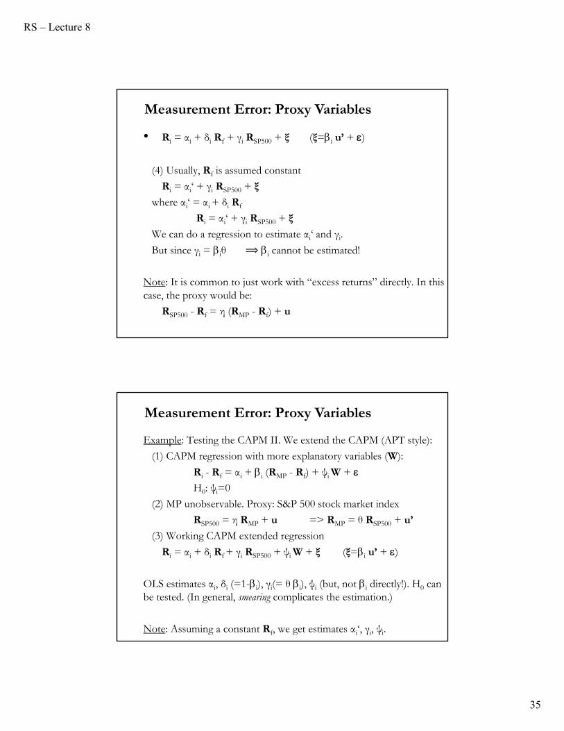
• Ri = αi + δi Rf + γi RSP500 + ξ (ξ=i u’ + )

(4) Usually, Rf is assumed constant

Ri = αi‘ + γi RSP500 + ξ

where αi‘ = αi + δi Rf

Ri = αi‘ + γi RSP500 + ξ

We can do a regression to estimate αi‘ and γi.

But since γi = iθ ⟹ i cannot be estimated!

Note: It is common to just work with “excess returns” directly. In this case, the proxy would be:

RSP500 - Rf = η (RMP - Rf) + u


Example: Testing the CAPM II. We extend the CAPM (APT style):

(1) CAPM regression with more explanatory variables (W):

Ri - Rf = αi + i (RMP - Rf) + ψi W + H0: ψi=0

(2) MP unobservable. Proxy: S&P 500 stock market index

RSP500 = η RMP + u => RMP = θ RSP500 + u’

(3) Working CAPM extended regression

Ri = αi + δi Rf + γi RSP500 + ψi W + ξ (ξ=i u’ + )

OLS estimates αi, δi (=1-i), γi(= θ i), ψi (but, not i directly!). H0 can be tested. (In general, smearing complicates the estimation.)

Note: Assuming a constant Rf, we get estimates αi‘, γi, ψi.


RS – Lecture 8

36

Measurement Error: Smearing Again (Greene)

1 1 2 2

1 1 1

2

1 2

M u ltip le re g re s s io n : y = x * x *

x * is m ea su re d w ith e rro r; x x * u

x is m ea su re d w ith o u t e rro r.

T h e re g re ss io n is e s tim a te d b y le a s t squ a re sPo pu la r m y th # 1 . b is b ia se d do w n w a rd , b co n s is te

ij i j

ij

n t.

P o pu la r m y th # 2 . A ll c o e ffic ie n ts a re b ia se d to w a rd ze ro .R e su lt fo r th e s im p le s t c a se . L e t

co v ( x * , x * ) , i, j 1 , 2 (2 x2 co va r ia n ce m a tr ix )

ijth e le m e n t o f th e in ve rse o f th e co va ria n ce m a tr ix

2

2 12

1 1 2 2 12 11 2 11

v a r(u)Fo r th e le a s t squ a re s e s tim a to rs :

1p lim b , p lim b

1 1

T h e e ffe c t is c a lle d "sm ea r in g ."

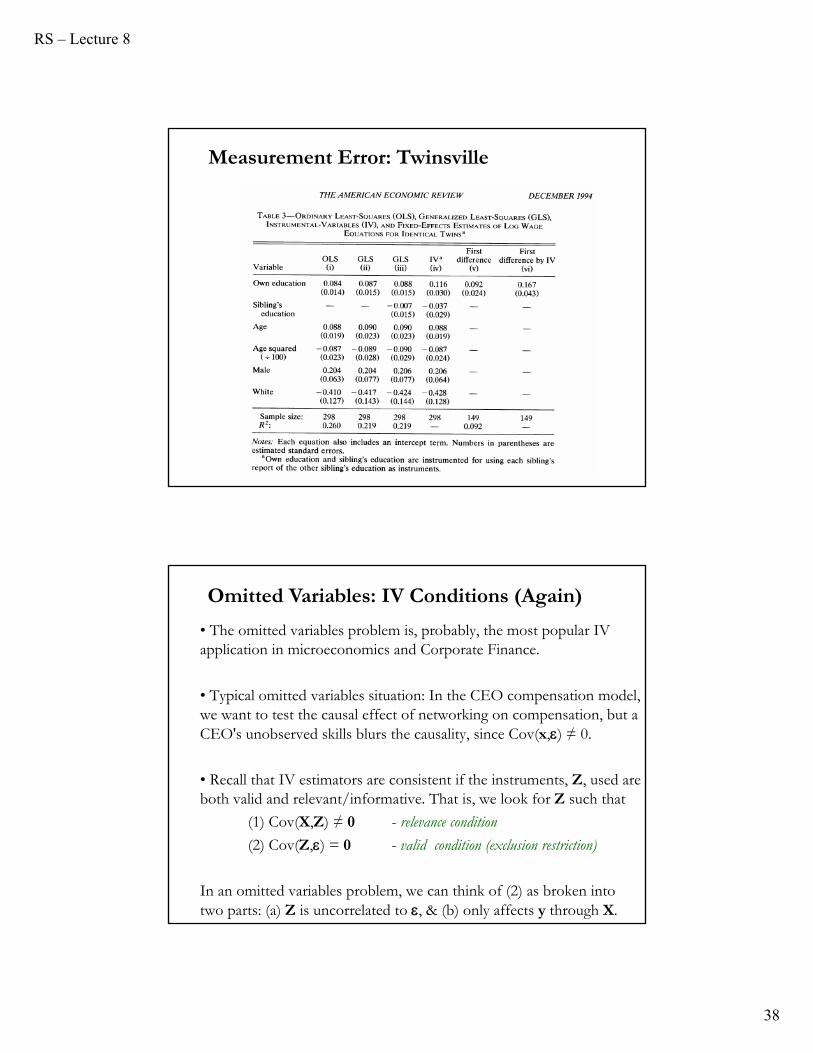
• Q: Does education affects earnings?

A: We expect two people with similar natural abilities but different levels of education to be differently paid. To estimate returns-to-schooling, economists often use a linear regression model relating log earnings (y) to years of education (x*), with additional control variables (U). The error term represents the effects of person-to-person variation that have not been controlled for. The DGP:

y = x* + Uγ + • We expect two people with similar natural abilities:

⟹ More education, more earnings. We expect >0.

• Problem: x* is usually self-reported, and often reported with error.

Measurement Error: Twinsville

RS – Lecture 8

37

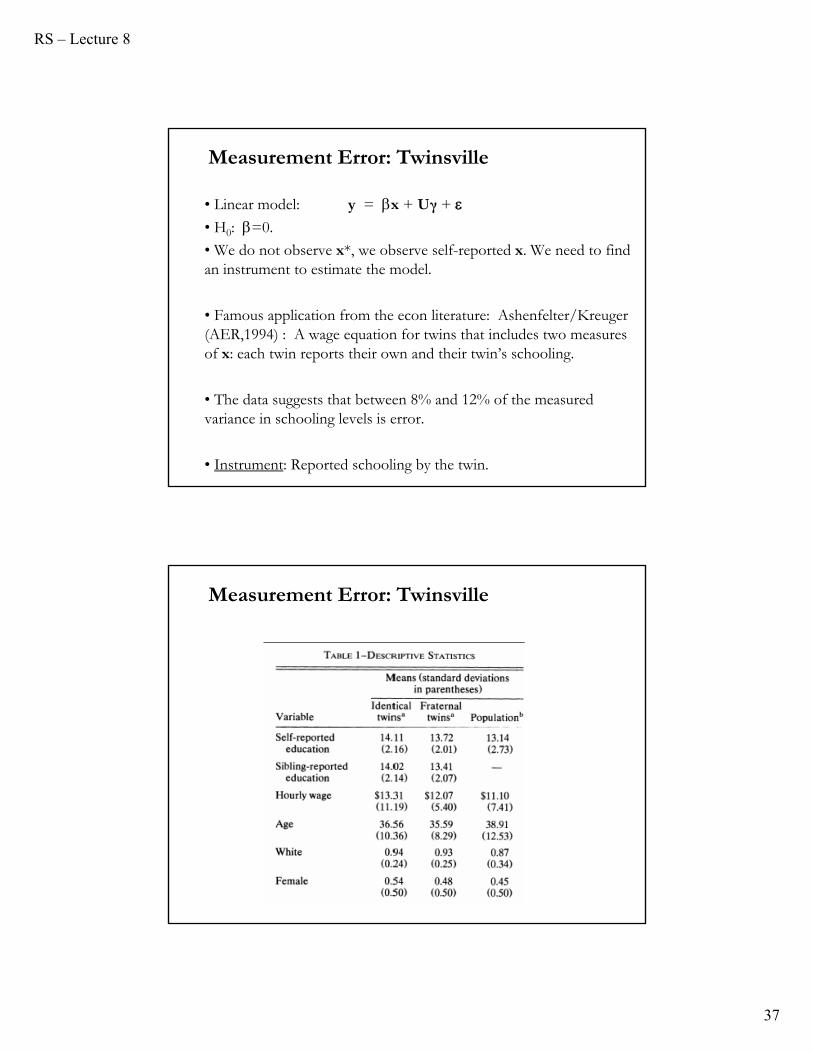
• Linear model: y = x + Uγ + • H0: =0.

• We do not observe x*, we observe self-reported x. We need to find an instrument to estimate the model.

• Famous application from the econ literature: Ashenfelter/Kreuger(AER,1994) : A wage equation for twins that includes two measures of x: each twin reports their own and their twin’s schooling.

• The data suggests that between 8% and 12% of the measured variance in schooling levels is error.

• Instrument: Reported schooling by the twin.



RS – Lecture 8

38


• The omitted variables problem is, probably, the most popular IV application in microeconomics and Corporate Finance.

• Typical omitted variables situation: In the CEO compensation model, we want to test the causal effect of networking on compensation, but a CEO's unobserved skills blurs the causality, since Cov(x,) ≠ 0.

• Recall that IV estimators are consistent if the instruments, Z, used are both valid and relevant/informative. That is, we look for Z such that

(1) Cov(X,Z) ≠ 0 - relevance condition

(2) Cov(Z,) = 0 - valid condition (exclusion restriction)

In an omitted variables problem, we can think of (2) as broken into two parts: (a) Z is uncorrelated to , & (b) only affects y through X.

Omitted Variables: IV Conditions (Again)

RS – Lecture 8

39

• (2) ⇒ Z is not only uncorrelated to , but only affects y through X –after all, it is excluded from structural equation! From the second part: Once I know the effect of Z on X, I can throw Z.

• That is, we have 3 requirements for Z to be a good IV:

- Z is correlated to X

- Z is as good as randomly assigned with respect to model.

- Z is an excluded instrument –i.e., it is not in structural equation.

• The relevant condition (the first requirement) is the only one we can directly check, through the first-stage regression, where we get .

• Given that is unobservable, the legitimacy of the valid condition (the last two requirements) is usually left for theory or common sense.


• Finding a Z that meets all requirements is not easy.

- Historically, the emphasis has been on the valid (exogeneity) condition, Cov(Z,)=0.

- But, the past 25 years added an additional source of concern: the Cov(X,Z) may not be high enough. That is, (from the first stage) may not be very informative about X:

X = ZП + Uδ + V – V ~N(0, σV2I)


RS – Lecture 8

40

• Back to CEO compensation model. We need IVs, Z, such that

(1) Explain the variation in networking –i.e., Cov(x,Z)≠0

(2) Do not directly affect CEO compensation –i.e., Cov(Z,)=0.

• It is not difficult to find a Z that meets (2), the valid condition. Many variables are not correlated with , the error term from the CEO compensation structural equation.

Examples: Potential IVs, uncorrelated with . Earthquakes in New Zealand; past debt of Denton, TX; asteroids hitting the Atlantic the year of the CEO’s birth; number of letters on the name of CEO’s high school.

• We like these potential IVs, they look random or orthogonal to a CEO compensation model (unrelated to ). They can be safely excluded from the structural equation. That is, they meet Cov(Z,)=0.

Omitted Variables: Finding Good IVs

• But, it is dubious the effect of these IVs on networking, x. The relevant condition is likely not met.

Note: Deaton (2010) calls the variables in the examples external, since they are not determined by the model. They may not be exogenous.

• The key is to find a Z correlated with X –i.e., the relevant condition–uncorrelated with (and with the omitted variable, unobserved skills.)

• Starting with Angrist (1990) and Angrist and Krueger (1991) (for us, A&K), who study the effect on earnings of civilian work experience and schooling, respectively, there has been an emphasis on using a Zthat can be defined by a natural experiment when the IV problem is caused by omitted variables.

• Usually, a natural experiment is exogenous to a structural model. Like the previous external examples, the exclusion condition is met.


RS – Lecture 8

41

• The key is to find a natural experiment (defining Z) that is correlated with X and has no direct effect on y –the impact on y is through X:

Z → X → y

Since Z is an exogenous event, the resulting values of X induced by Zmay be considered randomized.

• Recall that in the CEO compensation model, we want to test the causal effect of networking on compensation, but an omitted variable –the CEO's unobserved skills- creates endogeneity.

• A solution to the omitted variables problem is to assign networking (x) randomly: we have two similar groups of CEOs (with similar skills!) and randomly we assign them values (say, large network & small network). Of course, this randomized experiment is not possible.


• But, suppose we have a natural event, Z, unrelated to y, which randomly assigns X to two groups. Then, we can test causality, without the omitted variable problem.

• We use Z to identify causality. This is why natural experiments are popular in economics & finance (especially, in Corporate Finance).

• We define natural experiments as historical (exogenous) episodes that provide observable, quasi-random variation in treatment subject to a plausible identifying assumption.

• “Natural” point out that us (the researchers) did not design the episode to be analyzed, but can use it to identify causal relationships.

Omitted Variables: Natural Experiments

RS – Lecture 8

42

• A natural experiment defines an IV: Zi=1 (i treated), Zi=0 (i control).

• Now, we identify two groups: treated (all i with Zi=1) & control (all iwith Zi=0). Then, we analyze differences between the two groups (y(1), X(1)) and (y(0), X(0)).

• But, for our analysis to be treated like a lab experiment (the gold standard in experimental sciences), we need to show that the treatment is in fact randomly assigned. We need to show that two groups are comparable along all dimensions relevant for the outcome variable except the one involving the treatment.

• This is the key for the experiment to be valid. We need to convince the reader that the we have a quasi-random treatment.

Omitted Variables: Natural Experiments

• Example: There are significant persistent differences in development (y) among similar cities. One explanation: Location (x); proximity to other cities matter. Cities close to another city enjoy externalities (say, transportation and school networks). We want to test this hypothesis.

I would like to estimate a model: y = x + Uγ + (but location, x, is also endogenous. OLS will not work!)

- Ideal experiment: Identify 2 similar cities and remove a city next to it.

- Natural experiment: German division in 1949. Now, cities close to the border lost connection to the cities on the other side of the border. It looks like randomly removing a city! (from Redding & Sturm. 2008, AER).

Finding Good IVs: Natural Experiments

RS – Lecture 8

43

• Now, we need to convince the reader that the German division provides a legitimate quasi-random treatment:

- We need to show that the partition was exogenous (not based on development, y -i.e., unrelated to the structural model!)

- We need to show that there was no cofounding treatment (something else happening along with the partition). For example, after the partition, a city close to the border may be in fear of war.

Finding Good IVs: Natural Experiments

• IV estimators are consistent if the instruments, Z, used are both valid and relevant/informative, but they may be subject to significant finite sample biases.

• We now look at two distinct sources of finite sample bias:

- The use of IVs that are only weakly related to the endogenous variable(s), resulting in “weak identification” of the parameters of interest. This is the weak instruments problem.

- The use of “too many” instruments relative to the available sample size. This is the overidentification problem.

Finite Sample Problems

RS – Lecture 8

44

• The explanatory power of Z may not be enough to allow inference on . In this case, we say Z is a weak instrument.

Definition: Weak InstrumentIVs are weak if the mean component of X that depends on the IVs –ZП– is small relative to the variability of X, or equivalently, to the variability of the error V.

• Implications:

- Gleser and Hwang (1987) and Dufour (1997) show that CIs and tests based on t-tests and F (Wald) tests are not robust to weak IVs.

- The concern is not just theoretical: Numerical studies show that coverage rates of conventional 2SLS CIs can be very poor when IVs are weak, even if T is large.

Weak Instruments: Definition and Implications

• Usual detection of weak IVs: Check if H0 (weak instruments): П = 0:

- Test H0: П = 0 with a standard F-test on Z in the 1st stage regression.

- Look the partial-R2 (the exogenous variable U is partialed out).

Note: There is a theoretical problem when, under a H0, we have unidentified parameters. Under H0: П = 0, is not identified.

Weak Instruments: Detection

RS – Lecture 8

45

• Back to the question: Does education affect earnings?

We use the same linear model: y = x + Uγ + where we are interested in the effect of schooling (x) on log earnings (y). We expect >0. But, given that Cov(x,)≠0; we know that OLS inconsistent . We need IV estimation.

Note: In general, U does not capture much of the variation of y.

• Angrist and Krueger’s (1991, QJE) Natural experiment: Find an exogenous historical event that creates variation in schooling.

Exogenous event: Compulsory schooling laws according to age, not years of schooling completed.

Finding an Instrument: A&K (1991)

• Years of schooling vary by quarter of birth (QOB=z):

– In the U.S., it is legal to drop out at 16.

– Someone born in Q1 is a little older and can drop out with less schooling, than someone born in Q4 ⇒ Cov(z, x) ≠ 0.

• QOB can be treated as a source of exogeneity in schooling, unrelated to individual ability ⇒ Cov(z, ) = 0.

• That is, Z should affect earnings only through its effect on schooling.


RS – Lecture 8

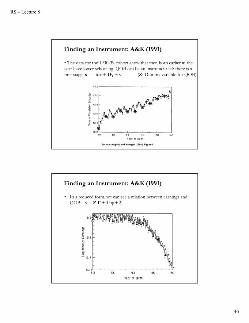
46

• The data for the 1930-39 cohort show that men born earlier in the year have lower schooling. QOB can be an instrument ⟹ there is a first stage: x = π z + Dγ + v (Z: Dummy variable for QOB)

Source: Angrist and Krueger (1991), Figure I


• In a reduced form, we can see a relation between earnings and QOB: y = Z Г + U φ + ξ


RS – Lecture 8

47

• People born in Q1 do obtain less schooling

– But pay close attention to the scale of the y-axis.

– Mean differences between Q1 and Q4 are small (in education, the difference is only 0.151 and in log earnings 0.014).

• Thus, we need large T since R2X,Z will be very small

– A&K had over 300,000 observations for the 1930-39 cohort

• Final 2SLS model interacted QOB with year of birth (30), state of birth (150):

– OLS: bOLS = .0628 (s.e. = .0003) (large T =>small SE’s).

– 2SLS: b2SLS = .0811 (s.e. = .0109)

– Var[bIV] > Var[bOLS], as expected. (But, maybe too large?)


• OLS estimate does not appear to be badly biased. But...


RS – Lecture 8

48

• True story: The graduate labor class at the University of Michigan does replication exercises. Two students, Regina Baker and David Jaeger replicated the results in Angrist and Krueger (1991).

• Two things bother them and their professor, John Bound:

(1) The results are imprecise and unstable when the controls and instrument sets change.

(2) The results become precise and stable only when the 1st stage Ftests cannot reject coefficients which are jointly zero –i.e., when instruments are not weak.

Note: Consider the first stage: X = ZП + ξ.

Even if П=0 in the DGP, as the number of instruments increases the R2 of the first stage regression in the sample can only increase.

Weak Instruments: A&K (1991)

Note: From BJB (1995, JASA). Different instruments deliver different 1st stage F-stats. In only (2) there is a significant F-stat!


RS – Lecture 8

49

Note: As the number of IVs increase, b2SLS gets closer to bOLS.


• BJB suspected the presence of irrelevant IV. Then, they estimated the IV coefficient with a randomly assigned Z so that π =0 by construction. They reproduced the OLS estimate.

⇒ BJB’s suggestion: look at the 1st stage F-stat.


RS – Lecture 8

50

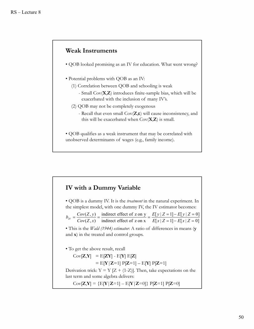
• QOB looked promising as an IV for education. What went wrong?

• Potential problems with QOB as an IV:

(1) Correlation between QOB and schooling is weak

- Small Cov(X,Z) introduces finite-sample bias, which will be exacerbated with the inclusion of many IV’s.

(2) QOB may not be completely exogenous

- Recall that even small Cov(Z,) will cause inconsistency, and this will be exacerbated when Cov(X,Z) is small.

• QOB qualifies as a weak instrument that may be correlated with unobserved determinants of wages (e.g., family income).

Weak Instruments

• QOB is a dummy IV. It is the treatment in the natural experiment. In the simplest model, with one dummy IV, the IV estimator becomes:

• This is the Wald (1944) estimator: A ratio of differences in means (yand x) in the treated and control groups.

• To get the above result, recall

Cov[Z,Y] = E[ZY] - E[Y] E[Z]

= E[Y|Z=1] P[Z=1] – E[Y] P[Z=1]

Derivation trick: Y = Y [Z + (1-Z)]. Then, take expectations on the last term and some algebra delivers:

Cov[Z,Y] = {E[Y|Z=1] – E[Y|Z=0]} P[Z=1] P[Z=0]

IV with a Dummy Variable

]0|[]1|[

]0|[]1|[

on x z ofeffect indirect

yon z ofeffect indirect

),(

),(

ZxEZxE

ZyEZyE

xZCov

yZCovbIV

RS – Lecture 8

51

• Similar work for Cov[X,Y] gets the result: bIV = Wald Estimator.

• Interpretation of Wald Estimator, as a ratio of slopes:

- First stage: x = π1 + π2 z + v

- Reduced form: y = γ1 + γ2 z + ξ

Taking conditional expectations on Z above and simple algebra:

π2 = E[x|Z=1] - E[x|Z=0]

γ2 = E[y|Z=1] - E[y|Z=0]

Then, 2

2

]0|[]1|[

]0|[]1|[

ZxEZxE

ZyEZyEbIV

• The Wald estimator is known as local IV or local average treatment effect, LATE (under some assumptions, bIV=E[y(1)-y(0)|compliers]).


• Application to A&K (1991):

bIV = (5.90271-5.8916)/(12.7969-12.6881) = 0.1021

Interpretation: The Wald estimator measures the effect of an extra year of schooling on those (dropout) students for whom an earlier birth –i.e., Z changes from 0 to 1– would have been forced to complete an extra year of schooling before dropping out.


RS – Lecture 8

52

• The above result can be extended to IV with multiple dummy instruments. For example, J categories; say, 4 QOB: Q1, Q2, Q3, Q4.

From the structural equation: yi = xi + i

=> E[yi |Zi] = E[xi|Zi]

• We replace the expectations (say, E[yi |Zi=j]) with sample analogs ( j). Then, in this case, the IV estimator is the same as the coefficient from a regression of J group means between Y and X , weighted by the size of the groups.


• Let’s go back to b2SLS = [Y' Pz Y]-1 Y'Pz y1

and look at the bias: E[b2SLS - ] = E[[Y' Pz Y]-1 (П'Z'+V') Pz ].This expectation is hard to evaluate because the expectation operator does not pass through the inverse [[Y' Pz Y]-1, a nonlinear function.

Trick: Group asymptotics. Still use an asymptotic argument but let

the number of instruments grow at the same rate as the sample size.

This “keeps the instruments weak.”

• Group asymptotics gives us something like an expectation, but we can take these expectations through non-linear functions:

E[b2SLS - ] ≈ E[[Y' Pz Y]-1] E[(П'Z' )]+ E[[Y' Pz Y]-1] E[V'Pz ]Since E[(П'Z' )]=0, E[b2SLS - ] ≈ E[[Y' Pz Y]-1] E[V'Pz ]

2SLS Bias with Many Instruments

RS – Lecture 8

53

• Substituting in the first stage: E[b2SLS - ] ≈ E[(П'Z'+V')' Pz (ZП+V)]-1 E[V'Pz ]

= E[[П'Z' ZП] + E[V'PzV]]-1 E[V'Pz ]

• Recall matrix algebra tricks: V'PzV is a scalar, thus it is equal to its trace; the trace is a linear operator which passes through expectations and is invariant to cyclic permutations; finally, the trace of Pz, an idempotent matrix, is equal to its rank, l. Then,

E[V'PzV] ≈ E[tr(V'PzV)] = E[tr(PzVV')] = tr(Pz E[( VV')] = tr(Pz σVV I) = σVV tr(Pz) = σVV l.

• Similar results applies to E[V'Pz ] = σεV l.

• Then, E[b2SLS - ] ≈ σεV l E[[П'Z' ZП] + σVV l ]-1


• Then, E[b2SLS - ] ≈ σεV l E[[П'Z' ZП] + σVV l]-1

= σεV /σVV E[[П'Z' ZП]/(σVV l )+1]-1

Note that F = [E[П'Z' ZП]/l ]/[σVV ] is the population F-statistic for H0: П=0 in the 1st stage regression. Thus,

E[b2SLS - ] ≈ σεV /σVV [1/(F+1)]

• Suppose the 1st stage coefficients, П, are zero. Then, F=0

⟹ E[b2SLS - ] ≈ σεV /σVV = σεV /σYY (OLS bias!)

Intuition: If П=0, then any variation in in the sample comes from V. The variation in is not different from the variation in X.

Note: This bias can affect tests, for example, the Hausman test.

X̂X̂


RS – Lecture 8

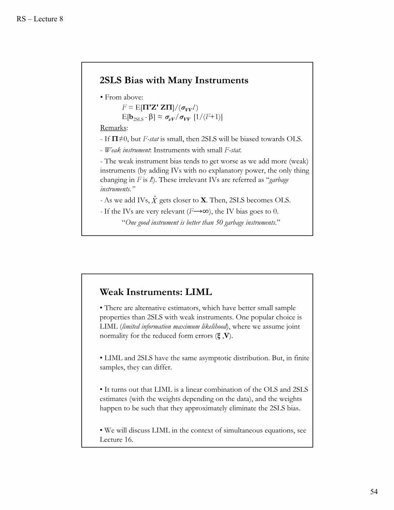
54

• From above: F = E[П'Z' ZП]/(σVV l ) E[b2SLS - ] ≈ σεV /σVV [1/(F+1)]

Remarks:

- If П≠0, but F-stat is small, then 2SLS will be biased towards OLS.

- Weak instrument: Instruments with small F-stat.

- The weak instrument bias tends to get worse as we add more (weak) instruments (by adding IVs with no explanatory power, the only thing changing in F is l!). These irrelevant IVs are referred as “garbage instruments.”

- As we add IVs, gets closer to X. Then, 2SLS becomes OLS.

- If the IVs are very relevant (F⟶∞), the IV bias goes to 0.

“One good instrument is better than 50 garbage instruments.”


X̂

• There are alternative estimators, which have better small sample properties than 2SLS with weak instruments. One popular choice is LIML (limited information maximum likelihood), where we assume joint normality for the reduced form errors (ξ ,V).

• LIML and 2SLS have the same asymptotic distribution. But, in finite samples, they can differ.

• It turns out that LIML is a linear combination of the OLS and 2SLS estimates (with the weights depending on the data), and the weights happen to be such that they approximately eliminate the 2SLS bias.

• We will discuss LIML in the context of simultaneous equations, see Lecture 16.

Weak Instruments: LIML

RS – Lecture 8

55

Weak Instruments: LIML

Example: The consumption CAPM.

After (many) assumptions, excess returns for a risky asset are a (linear) function of the covariance of the asset’s returns with consumption growth:

Et [rt+1] – rf = γσrΔ - σr2/2

where rt+1= ln(1+Rt+1) - Rt+1: return on a risky asset.σr

2 = Var[ln(1+Rt+1)] = Var(rt+1)σΔ2 = Var[ln(ct+1) - ln(ct)] σrΔ = Cov[ln(ct+1) - ln(ct), rt+1]γ = Risk aversion coefficient from a CRRA utility function.

• The C-CAPM is easy to test using linear regressions.

• There is also a non-linear version of the C-CAPM.

Weak Instruments: Finance application

RS – Lecture 8

56

• In both linear and nonlinear versions of the model, IVs are weak --see Neeley, Roy, and Whiteman (2001), and Yogo (2004).

• In the linear model in Yogo (2004):

X (endogenous variable): consumption growth

Z (the IVs): twice lagged nominal interest rates, inflation, consumption growth, and log dividend-price ratio.

• But, log consumption is close to a random walk, consumption growth is difficult to predict. This leads to the IVs being weak.

⟹ Yogo (2004) finds F-statistics for H0: П = 0 in the 1st stage regression that lie between 0.17 and 3.53 for different countries.

Weak Instruments: Finance application

• Symptom: The relevance condition, plim(Z’X/T )≠0, is close to being violated.

• Detection of weak IV:

– Rule of thumb: For a single endogeneous regressor, Staiger and Stock (1997) suggest that 1st stage F < 10 is cause for concern.

– Low partial-R2X,Z –see, Shea (1997).

– Large Var[bIV].

• Remedy:

– Not much – most of the discussion is about the condition, not what to do about it.

– Pick your best instrument and report just-identified results.

– Use LIML? Requires a normality assumption. Probably, not too restrictive.

Weak Instruments: Detection and Remedies

RS – Lecture 8

57

• Symptom: The valid condition, plim(Z’ε/T )=0, is close to being violated. Since the errors are not observed, very difficult to check.

• The valid condition is an exclusion restriction on the model:y = Y + Z + Y = Z П + V

⟹ The exclusion restriction imposes H0: = 0.

• If the exclusion is incorrect –i.e., θ = θ0 0 –, will show an omitted variables bias problem. In the simple one exogenous variable & one IV case, it is easy calculate the bias:

bIV = β + θ0/

The smaller , the bigger the bias (the bias is worse with weak IVs).


• Detection of instrument exogeneity:

– Endogenous IV’s: Inconsistency of bIV that makes it no better (and probably worse) than bOLS.

– Durbin-Wu-Hausman test: Endogeneity of the problem regressor(s). But, DWH tests do not have good properties in the presence of weak instruments.

• Remedy:

– Some modifications of the DWH have been suggested under weak instruments, see Hahn and Hausman (2002, 2005).

– Avoid endogeneous weak instruments.

– General problem: It is not easy to find good instruments in theory and in practice. Find natural experiments.


RS – Lecture 8

58

Weak Instruments: Testing

• Irrelevant IVs –i.e., П=0– and weak IVs bias the IV estimation. Weak IVs the presence of weak instruments, conventional asymptotics fail (see, Staiger and Stock (1997).

• Small simulation (replications = 2,000).

- Simple case: one endogenous variable, one IV. ParametersZ, , V ~ N(0, Σ .Set unit variances, but Cov(,V)=ρ=1; l=1 & 5; T = 100 & 1,000; ρ = .99 & .30

- Compute t =(b2SLS – 1)/SE(b2SLS) - We determine empirical size of 5% t-test (check|t2SLS|>1.96)- We study 3 cases:1) Strong instruments (when l=1, π = 1; when l=5, π’ = [1 1 0 0 0])2) Weak instruments (when l=1, π = .1; when l=5, π’ = [.1 .1 0 0 0])3) Irrelevant instruments π 0 (approximated by .0001)


Empirical size of 5% t-test (b2SLS )T = 100 T = 100

Quality of IV l=1 (ρ=.99) l=1 (ρ=.30) l=5( ρ=.99) l=5 (ρ=.30)

Strong .065 (0.99) .044 (1.00) .088 (1.02) .051 (1.01)

Weak .195 (1.31) .006 (2.26) .852 (1.70) .057 (1.22)

Irrelevant .633 (2.01) .001 (1.40) .995 (1.99) .045 (1.28)

Empirical size of 5% t-test (b2SLS )T = 1,000 T = 1,000

Quality of IV l=1 (ρ=.99) l=1 (ρ=.30) l=5( ρ=.99) l=5 (ρ=.30)

Strong .051 (1.00) .002 (1.00) .049 (1.00) .050 (1.00)

Weak .093 (0.79) .002 (0.93) .257 (1.13) .059 (1.05)

Irrelevant .631 (2.01) .004 (0.60) .995 (1.99) .043 (1.31)

RS – Lecture 8

59


• In the presence of weak IVs, the usual tests have size problems. They are also not asymptotically pivotal: the distribution depends on nuisance parameters (ρ,П) that cannot be consistently estimated.

• Anderson and Rubin (1949) propose a test of H0: =0, the AR stat, an F-test, that has good properties under the usual situations encountered under IV estimation.

• Intuition of AR test. - Subtract from model Y0:

y - Y0 = Y - Y0 + = Y ( - 0 ) + - Substitute 1st stage:

y - Y0 = (ZП+V) (-0 ) + = ZП (-0 ) + V (- 0 ) + = ZΦ+ W


y - Y0= ZΦ + W

where

Φ П (-0 )

W = V (- 0 ) + Now, we can estimate Φ using OLS, since Z is uncorrelated with W.

Note that testing H0: Φ=0 ⟹ H0: =0

• The AR stat is the usual F-stat for testing Φ=0. Under the usual assumptions (fixed regressors and normal errors), the AR stat follows the usual F distribution.

• Under weak instruments –see Staiger and Stock (1997):

l ∙AR = l ∙F(Φ=0) →χ2(l).

RS – Lecture 8

60


Note:

- Note that under H0: =0, the F-stat does not depend on П.

- The AR test is a joint test. It tests the joint hypothesis =0 and Z is uncorrelated with .

• It turns out that the power of the AR test is not very good when l>1. The AR test tests whether Z enters the (y - Y0) equation. The AR test sacrifices power: It ignores the restriction Φ П (-0 ).

• Low power leads to very wide CIs based on such tests. Kleibergen (2002) and Moreira (2001) propose an LM test whose H0 rate is robust to weak IVs. (LM test first estimates П under H0:=0.)


• There is an interesting literature on constructing CI under garbage instruments. That is, CI that are robust to the presence of weak and irrelevant instruments. See Staiger and Stock (1997) and Kleibergen (2002, 2003).

Example: It is possible to invert the AR stat to get a weak instrument robust CI interval for :

CIα = {0 : l ∙AR ≤ χ2α (l)}

RS – Lecture 8

61

• If one uses an F-test to detect weak IVs as a pre-test procedure, then the usual pre-testing issues arise for subsequent inference --see Hall, Rudebusch, and Wilcox (1996).

• In practice, researchers do tend to inspect and report the strength of the first stage. Tests and CI will not have the appropriate nominal size.

• Chioda and Jansson (2006) propose a similar statistic to the AR-stat to build a C.I.. It has a non-standard distribution conditional on the 1st stage F-stat. The C.I. are wider than the ones that do not condition on the 1st stage.

Weak Instruments: Pre-testing

• Situation: l is much larger than k. Possible “overidentification.”

• Extreme case: Suppose l =T. In this case, Z is a square matrix:

b2SLS = [W'Z'X]-1 W'Z'y = [X'Z(Z’Z)-1Z’X ]-1 X'Z(Z’Z)-1Z’y

= [X'Z Z-1 Z'-1 Z’X ]-1 X'Z Z-1 Z'-1 Z’y = [X'X ]-1 X'y = b

Since b is inconsistent and biased when E[ε|X]≠0, then so is b2SLS.

• While nobody will set l=T, a similar finite sample bias occurs in less extreme cases. In general, as l →T, we see that b2SLS →bOLS.

Note: For the IV asymptotic theory to be a good approximation, Tmust be much larger than l (say, T - l > 40 & grow linearly with T.)

Excessive Overidentification

RS – Lecture 8

62

• Angrist and Pischke (2009) report that “just-identified 2SLS is approximately unbiased.” They report a simulation with weak IVs, using OLS, just-identified IV and 2SLS with 20 IVs (and LIML too):


• Angrist and Pischke (2009) also report coverage rates of 95% C.I. (The coverage rate is the probability that a C.I. includes the true parameter.) Coverage rates for OLS and 2SLS are poor.

• Using lots of instruments can bias estimation (too many weak instruments) and cause innacurate asymptotic approximations.


RS – Lecture 8

63

• Obvious symptom: Z has many more columns than X

- 1st stage of 2SLS almost reproduces X

- 2d stage of 2SLS becomes OLS, which is biased.

• Detection:

- Visual – there is no test.

- Check b2SLS and bOLS. It they are similar, check that this is not a result of “too many IVs.”

• Remedy:

- Fewer instruments? (Several methodological problems with this idea). Donald and Newey (2001) consider this option.

- Jackknife estimation –see Ackerberg and Devereux (2009).

Excessive Overidentification (Greene)

• Finding good instruments –i.e., meet both conditions- is not easy.

• When only the relevant condition is emphasized, OLS can be better than IV (“the cure can be worse...”). Even “clever” IVs can have low correlations with X and create severe finite-sample bias. The bias tends to be worse when there are many overidentifying restrictions (l is large relative to k).

• For the simple case of one endogeneous variable, the F-stat in the 1st stage can help to identify weak IVs. When there are many IVs, Stock and Yogo (2005) provide rules of thumb regarding the weakness of instruments based on a statistic due to Cragg and Donald (1993).

IV: Remarks

RS – Lecture 8

64

• Large T will not help. A&K and Consumption CAPM tests have very large samples!

• Just identified IV is approximately unbiased (or less biased) even with weak instruments (although it is not possible to see this from the bias formula.)

IV: Remarks

What should you do in practice? (Pischke)

• Report first stage and think about whether it makes sense. Are the magnitude and sign as you would expect?

• Report the F-stat on the excluded IVs. The bigger this is, the better. Fs above 10 to 20 are considered relatively safe, lower Fs put you in the danger zone.

• Pick your best single IV and report just-identified estimates using this one only. Just-identified IV is approximately median-unbiased.

• Check over-identified 2SLS estimates with LIML. If the LIML

estimates are very different, or SEs are much bigger, worry.

• Check coefficients, t-stats, and F-stats for excluded IVs in the reduced-form regression of dependent variables on IVs. The reduced-form estimates are just OLS, so they are unbiased. If the relationship you expect is not in the reduced form, it is probably not there.

RS – Lecture 8

65

IV: Final General Remarks

• Finding good instruments is not easy. A good natural experiment, which defines the IV, is worthy of a paper.

• Angrist: “Tell a story about why a particular IV is a good instrument.” In the omitted variable case: “Does the IV, for all intents and purposes, randomize the endogenous regressor?”

• IV models can be very informative, but it is your job (as author of the paper) to convince the audience.

• Good IV models are generally interesting in their own right, and should not be treated as “robustness” checks.


• The emphasis on IV with natural experiments is part of the quasi-experimental revolution, which shifted the emphasis in mainly microeconomics from theory to empirical experiments: “From Mas-Colell to Angrist and Pischke.”

• Criticism to IV estimation using natural experiments:

- No theory. For example, there is no optimizing labor (structural) model behind A&K (1991). Q: Where does the reduced form equation come from?

- Difficult to interpret the results. For example, LATE is an average, which may or may not contain information about the parameter of interest. It may not be useful (see Heckman and Urzua (2009), for an example, where LATE is not informative).

RS – Lecture 8

66


• Answer from natural experimentalists to the criticism: Big skepticism about structural models. Thus, no modeling is good! Angrist and Pischke (2010): The explosion of IV methods, including LATE estimation, has led to greater “credibility” in applied econometrics.

• References:

- “Mostly Harmless Econometrics: An Empiricist's Companion,” textbook by Angrist and Pischke (2009).

- “Instruments, Randomization, and Learning about Development,” by Deaton (2010, JEL).

- “The Empirical Economist's Toolkit: From Models to Methods,” by Panhans and Singleton (2015, Duke Working Paper).

Lecture 8 Instrumental Variables - Bauer College of Business · PDF fileRS – Lecture 8 1...

Documents

Transcript of Lecture 8 Instrumental Variables - Bauer College of Business · PDF fileRS – Lecture 8 1...