Lecture 5: Model-Free Predictionjosephmodayil.com/UCLRL/MC-TD.pdf · Lecture 5: Model-Free...
50
Lecture 5: Model-Free Prediction Lecture 5: Model-Free Prediction Joseph Modayil
Transcript of Lecture 5: Model-Free Predictionjosephmodayil.com/UCLRL/MC-TD.pdf · Lecture 5: Model-Free...
Lecture 5: Model-Free Prediction
Lecture 5: Model-Free Prediction
Joseph Modayil

Lecture 5: Model-Free Prediction
Outline
1 Introduction
2 Monte-Carlo Learning
3 Temporal-Difference Learning
4 TD(λ)
Reading: (Sutton & Barto Oct 2015) Chapters 5, 6, and 7 onprediction
Lecture 5: Model-Free Prediction
Introduction
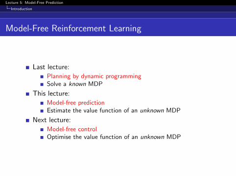
Model-Free Reinforcement Learning
Last lecture:
Planning by dynamic programmingSolve a known MDP
This lecture:
Model-free predictionEstimate the value function of an unknown MDP
Next lecture:
Model-free controlOptimise the value function of an unknown MDP
Lecture 5: Model-Free Prediction
Monte-Carlo Learning
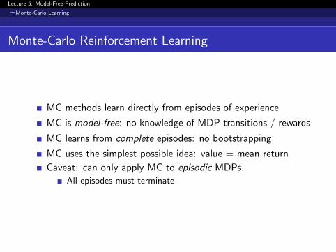
Monte-Carlo Reinforcement Learning
MC methods learn directly from episodes of experience
MC is model-free: no knowledge of MDP transitions / rewards
MC learns from complete episodes: no bootstrapping
MC uses the simplest possible idea: value = mean return
Caveat: can only apply MC to episodic MDPs
All episodes must terminate
Lecture 5: Model-Free Prediction
Monte-Carlo Learning
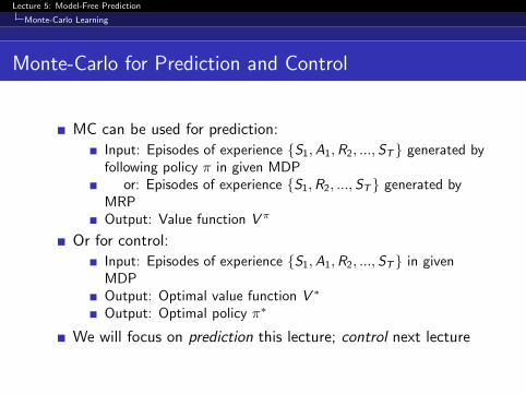
Monte-Carlo for Prediction and Control
MC can be used for prediction:
Input: Episodes of experience {S1,A1,R2, ...,ST} generated byfollowing policy π in given MDP
or: Episodes of experience {S1,R2, ...,ST} generated byMRPOutput: Value function V π
Or for control:
Input: Episodes of experience {S1,A1,R2, ...,ST} in givenMDPOutput: Optimal value function V ∗
Output: Optimal policy π∗
We will focus on prediction this lecture; control next lecture
Lecture 5: Model-Free Prediction
Monte-Carlo Learning
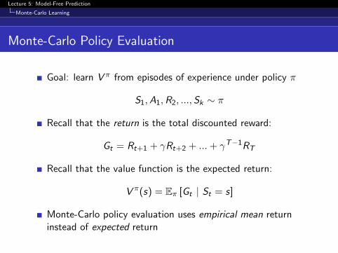
Monte-Carlo Policy Evaluation
Goal: learn V π from episodes of experience under policy π
S1,A1,R2, ...,Sk ∼ π
Recall that the return is the total discounted reward:
Gt = Rt+1 + γRt+2 + ...+ γT−1RT
Recall that the value function is the expected return:
V π(s) = Eπ [Gt | St = s]
Monte-Carlo policy evaluation uses empirical mean returninstead of expected return

Lecture 5: Model-Free Prediction
Monte-Carlo Learning
First-Visit Monte-Carlo Policy Evaluation
To evaluate state s
The first time-step t that state s is visited in an episode,
Increment counter N(s)← N(s) + 1
Accumulate total return M(s)← M(s) + Gt
Value is estimated by mean return V (s) = M(s)/N(s)
By law of large numbers, V (s)→ V π(s) as N(s)→∞
Lecture 5: Model-Free Prediction
Monte-Carlo Learning
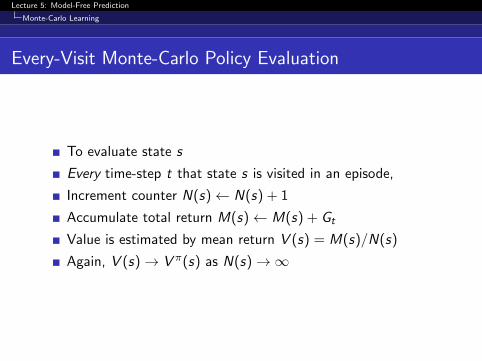
Every-Visit Monte-Carlo Policy Evaluation
To evaluate state s
Every time-step t that state s is visited in an episode,
Increment counter N(s)← N(s) + 1
Accumulate total return M(s)← M(s) + Gt
Value is estimated by mean return V (s) = M(s)/N(s)
Again, V (s)→ V π(s) as N(s)→∞
Lecture 5: Model-Free Prediction
Monte-Carlo Learning
Blackjack Example
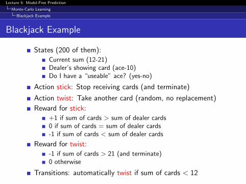
Blackjack Example
States (200 of them):
Current sum (12-21)Dealer’s showing card (ace-10)Do I have a “useable” ace? (yes-no)
Action stick: Stop receiving cards (and terminate)
Action twist: Take another card (random, no replacement)
Reward for stick:
+1 if sum of cards > sum of dealer cards0 if sum of cards = sum of dealer cards-1 if sum of cards < sum of dealer cards
Reward for twist:
-1 if sum of cards > 21 (and terminate)0 otherwise
Transitions: automatically twist if sum of cards < 12

Lecture 5: Model-Free Prediction
Monte-Carlo Learning
Blackjack Example
Blackjack Value Function after Monte-Carlo Learning
Policy: stick if sum of cards ≥ 20, otherwise twist
Lecture 5: Model-Free Prediction
Monte-Carlo Learning
Incremental Monte-Carlo
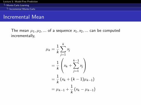
Incremental Mean
The mean µ1, µ2, ... of a sequence x1, x2, ... can be computedincrementally,
µk =1
k
k∑j=1
xj
=1
k
xk +k−1∑j=1
xj
=
1
k(xk + (k − 1)µk−1)
= µk−1 +1
k(xk − µk−1)
Lecture 5: Model-Free Prediction
Monte-Carlo Learning
Incremental Monte-Carlo
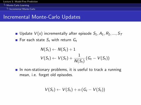
Incremental Monte-Carlo Updates
Update V (s) incrementally after episode S1,A1,R2, ...,ST
For each state St with return Gt
N(St)← N(St) + 1
V (St)← V (St) +1
N(St)(Gt − V (St))
In non-stationary problems, it is useful to track a runningmean, i.e. forget old episodes.
V (St)← V (St) + α (Gt − V (St))
Lecture 5: Model-Free Prediction
Temporal-Difference Learning
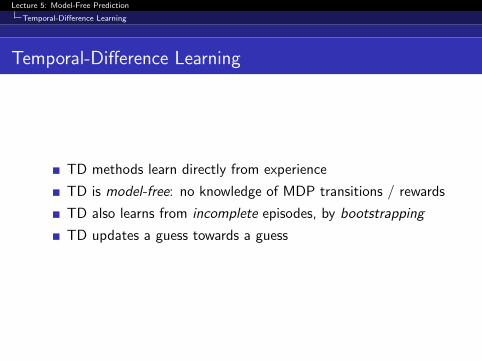
Temporal-Difference Learning
TD methods learn directly from experience
TD is model-free: no knowledge of MDP transitions / rewards
TD also learns from incomplete episodes, by bootstrapping
TD updates a guess towards a guess
Lecture 5: Model-Free Prediction
Temporal-Difference Learning
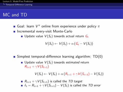
MC and TD
Goal: learn V π online from experience under policy π
Incremental every-visit Monte-Carlo
Update value V (St) towards actual return Gt
V (St)← V (St) + α (Gt − V (St))
Simplest temporal-difference learning algorithm: TD(0)
Update value V (St) towards estimated returnRt+1 + γV (St+1)
V (St)← V (St) + α (Rt+1 + γV (St+1)− V (St))
Rt+1 + γV (St+1) is called the TD targetδt = Rt+1 + γV (St+1)− V (St) is called the TD error
Lecture 5: Model-Free Prediction
Temporal-Difference Learning
Driving Home Example
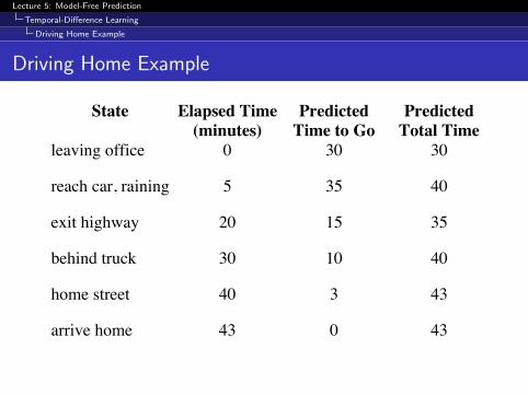
Driving Home Example
State Elapsed Time(minutes)
PredictedTime to Go
PredictedTotal Time
leaving office 0 30 30
reach car, raining 5 35 40
exit highway 20 15 35
behind truck 30 10 40
home street 40 3 43
arrive home 43 0 43
Lecture 5: Model-Free Prediction
Temporal-Difference Learning
Driving Home Example
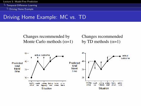
Driving Home Example: MC vs. TD
Changes recommended by Monte Carlo methods (!=1)!
Changes recommended!by TD methods (!=1)!
Lecture 5: Model-Free Prediction
Temporal-Difference Learning
Driving Home Example
Advantages and Disadvantages of MC vs. TD
TD can learn before knowing the final outcome
TD can learn online after every stepMC must wait until end of episode before return is known
TD can learn without the final outcome
TD can learn from incomplete sequencesMC can only learn from complete sequencesTD works in continuing (non-terminating) environmentsMC only works for episodic (terminating) environments
Lecture 5: Model-Free Prediction
Temporal-Difference Learning
Driving Home Example
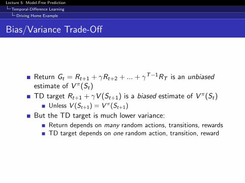
Bias/Variance Trade-Off
Return Gt = Rt+1 + γRt+2 + ...+ γT−1RT is an unbiasedestimate of V π(St)
TD target Rt+1 + γV (St+1) is a biased estimate of V π(St)
Unless V (St+1) = V π(St+1)
But the TD target is much lower variance:
Return depends on many random actions, transitions, rewardsTD target depends on one random action, transition, reward
Lecture 5: Model-Free Prediction
Temporal-Difference Learning
Driving Home Example
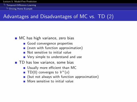
Advantages and Disadvantages of MC vs. TD (2)
MC has high variance, zero bias
Good convergence properties(even with function approximation)Not sensitive to initial valueVery simple to understand and use
TD has low variance, some bias
Usually more efficient than MCTD(0) converges to V π(s)(but not always with function approximation)More sensitive to initial value
Lecture 5: Model-Free Prediction
Temporal-Difference Learning
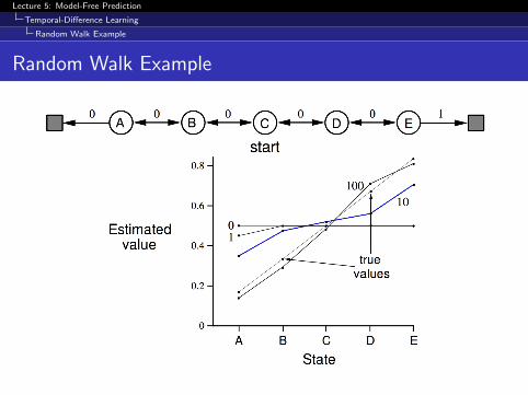
Random Walk Example
Random Walk Example

Lecture 5: Model-Free Prediction
Temporal-Difference Learning
Random Walk Example
Random Walk: MC vs. TD
Lecture 5: Model-Free Prediction
Temporal-Difference Learning
Batch MC and TD
Batch MC and TD
MC and TD converge: V (s)→ V π(s) as experience →∞and α→ 0
But what about batch solution for finite experience?
s11 , a
11, r
12 , ..., s
1T1
...
sK1 , aK1 , r
K2 , ..., s
KTK
e.g. Repeatedly sample episode k ∈ [1,K ]Apply MC or TD(0) to episode k
Lecture 5: Model-Free Prediction
Temporal-Difference Learning
Batch MC and TD
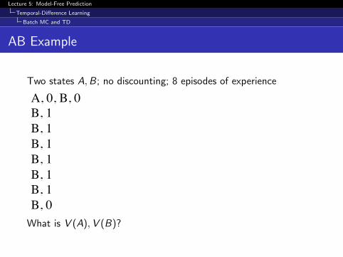
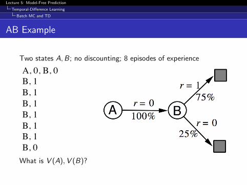
AB Example
Two states A,B; no discounting; 8 episodes of experience
A, 0, B, 0!B, 1!B, 1!B, 1!B, 1!B, 1!B, 1!B, 0!
What is V (A),V (B)?
Lecture 5: Model-Free Prediction
Temporal-Difference Learning
Batch MC and TD
AB Example
Two states A,B; no discounting; 8 episodes of experience
A, 0, B, 0!B, 1!B, 1!B, 1!B, 1!B, 1!B, 1!B, 0!
What is V (A),V (B)?
Lecture 5: Model-Free Prediction
Temporal-Difference Learning
Batch MC and TD
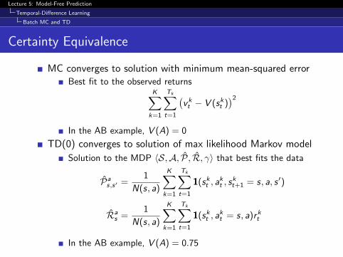
Certainty Equivalence
MC converges to solution with minimum mean-squared errorBest fit to the observed returns
K∑k=1
Tk∑t=1
(vkt − V (skt )
)2
In the AB example, V (A) = 0
TD(0) converges to solution of max likelihood Markov model
Solution to the MDP 〈S,A, P̂, R̂, γ〉 that best fits the data
P̂as,s′ =
1
N(s, a)
K∑k=1
Tk∑t=1
1(skt , akt , s
kt+1 = s, a, s ′)
R̂as =
1
N(s, a)
K∑k=1
Tk∑t=1
1(skt , akt = s, a)rkt
In the AB example, V (A) = 0.75
Lecture 5: Model-Free Prediction
Temporal-Difference Learning
Batch MC and TD
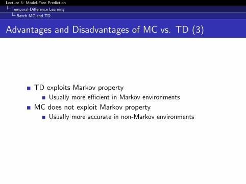
Advantages and Disadvantages of MC vs. TD (3)
TD exploits Markov property
Usually more efficient in Markov environments
MC does not exploit Markov property
Usually more accurate in non-Markov environments
Lecture 5: Model-Free Prediction
Temporal-Difference Learning
Unified View
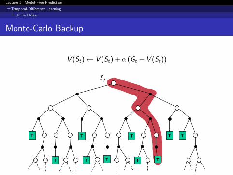
Monte-Carlo Backup
V (St)← V (St) + α (Gt − V (St))
T! T! T! T!T!
T! T! T! T! T!
st
T! T!
T! T!
T!T! T!
T! T!T!
Lecture 5: Model-Free Prediction
Temporal-Difference Learning
Unified View
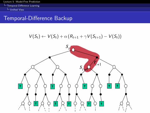
Temporal-Difference Backup
V (St)← V (St) + α (Rt+1 + γV (St+1)− V (St))
T! T! T! T!T!
T! T! T! T! T!
st+1rt+1
st
T!T!T!T!T!
T! T! T! T! T!
Lecture 5: Model-Free Prediction
Temporal-Difference Learning
Unified View
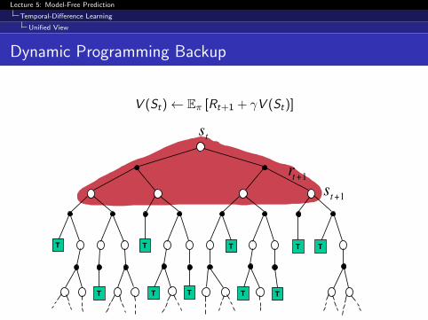
Dynamic Programming Backup
V (St)← Eπ [Rt+1 + γV (St)]
T!
T! T! T!
st
rt+1st+1
T!
T!T!
T!
T!T!
T!
T!
T!
Lecture 5: Model-Free Prediction
Temporal-Difference Learning
Unified View
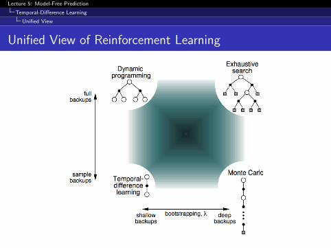
Bootstrapping and Sampling
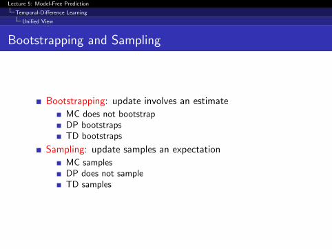
Bootstrapping: update involves an estimate
MC does not bootstrapDP bootstrapsTD bootstraps
Sampling: update samples an expectation
MC samplesDP does not sampleTD samples
Lecture 5: Model-Free Prediction
Temporal-Difference Learning
Unified View
Unified View of Reinforcement Learning
Lecture 5: Model-Free Prediction
TD(λ)
n-Step TD
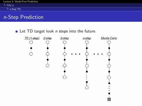
n-Step Prediction
Let TD target look n steps into the future
Lecture 5: Model-Free Prediction
TD(λ)
n-Step TD
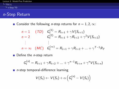
n-Step Return
Consider the following n-step returns for n = 1, 2,∞:
n = 1 (TD) G(1)t = Rt+1 + γV (St+1)
n = 2 G(2)t = Rt+1 + γRt+2 + γ2V (St+2)
......
n =∞ (MC ) G(∞)t = Rt+1 + γRt+2 + ...+ γT−1RT
Define the n-step return
G(n)t = Rt+1 + γRt+2 + ...+ γn−1Rt+n + γnV (St+n)
n-step temporal-difference learning
V (St)← V (St) + α(G
(n)t − V (St)
)
Lecture 5: Model-Free Prediction
TD(λ)
n-Step TD
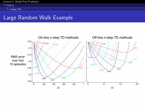
Large Random Walk Example
7.1. N -STEP TD PREDICTION 151
in Figure 6.5. Suppose the first episode progressed directly from the center state,C, to the right, through D and E, and then terminated on the right with a returnof 1. Recall that the estimated values of all the states started at an intermediatevalue, V (s) = 0.5. As a result of this experience, a one-step method would changeonly the estimate for the last state, V (E), which would be incremented toward 1, theobserved return. A two-step method, on the other hand, would increment the valuesof the two states preceding termination: V (D) and V (E) both would be incrementedtoward 1. A three-step method, or any n-step method for n > 2, would incrementthe values of all three of the visited states toward 1, all by the same amount.
Which value of n is better? Figure 7.2 shows the results of a simple empirical testfor a larger random walk process, with 19 states (and with a �1 outcome on the left,all values initialized to 0), which we use as a running example in this chapter. Resultsare shown for on-line and o↵-line n-step TD methods with a range of values for n and↵. The performance measure for each algorithm and parameter setting, shown on thevertical axis, is the square-root of the average squared error between its predictions atthe end of the episode for the 19 states and their true values, then averaged over thefirst 10 episodes and 100 repetitions of the whole experiment (the same sets of walkswere used for all methods). First note that the on-line methods generally worked beston this task, both reaching lower levels of absolute error and doing so over a largerrange of the step-size parameter ↵ (in fact, all the o↵-line methods were unstable for ↵much above 0.3). Second, note that methods with an intermediate value of n workedbest. This illustrates how the generalization of TD and Monte Carlo methods to n-step methods can potentially perform better than either of the two extreme methods.
On-line n-step TD methods Off-line n-step TD methods
↵↵
RMS errorover first
10 episodes
n=1
n=2
n=4n=8n=16
n=32
n=64256
128512
n=3n=64
n=1
n=2n=4
n=8
n=16
n=32
n=32n=64128512256
Figure 7.2: Performance of n-step TD methods as a function of ↵, for various values of n,on a 19-state random walk task (Example 7.1).
Exercise 7.1 Why do you think a larger random walk task (19 states instead of5) was used in the examples of this chapter? Would a smaller walk have shifted theadvantage to a di↵erent value of n? How about the change in left-side outcome from
Lecture 5: Model-Free Prediction
TD(λ)
n-Step TD
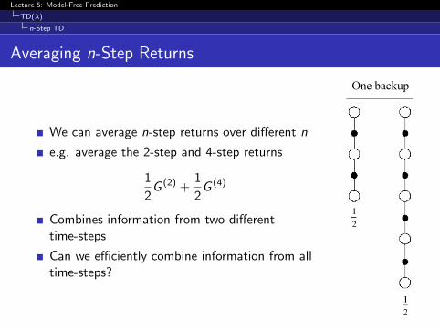
Averaging n-Step Returns
We can average n-step returns over different n
e.g. average the 2-step and 4-step returns
1
2G (2) +
1
2G (4)
Combines information from two differenttime-steps
Can we efficiently combine information from alltime-steps?
One backup
Lecture 5: Model-Free Prediction
TD(λ)
Forward View of TD(λ)
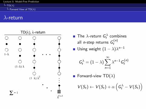
λ-return
The λ-return Gλt combines
all n-step returns G(n)t
Using weight (1− λ)λn−1
Gλt = (1− λ)
∞∑n=1
λn−1G(n)t
Forward-view TD(λ)
V (St)← V (St) + α(Gλt − V (St)
)
Lecture 5: Model-Free Prediction
TD(λ)
Forward View of TD(λ)
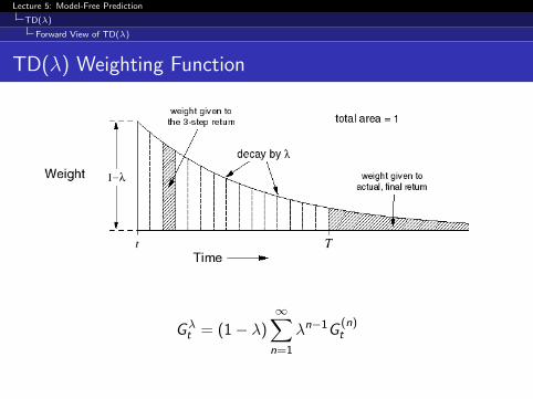
TD(λ) Weighting Function
Gλt = (1− λ)
∞∑n=1
λn−1G(n)t
Lecture 5: Model-Free Prediction
TD(λ)
Forward View of TD(λ)
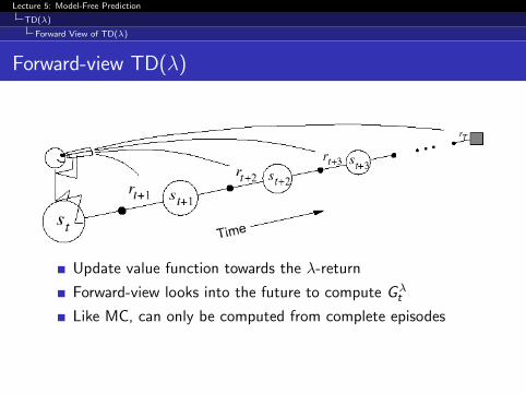
Forward-view TD(λ)
Update value function towards the λ-return
Forward-view looks into the future to compute Gλt
Like MC, can only be computed from complete episodes
Lecture 5: Model-Free Prediction
TD(λ)
Backward View of TD(λ)
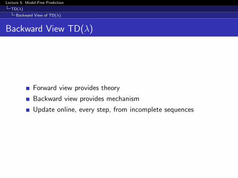
Backward View TD(λ)
Forward view provides theory
Backward view provides mechanism
Update online, every step, from incomplete sequences
Lecture 5: Model-Free Prediction
TD(λ)
Backward View of TD(λ)
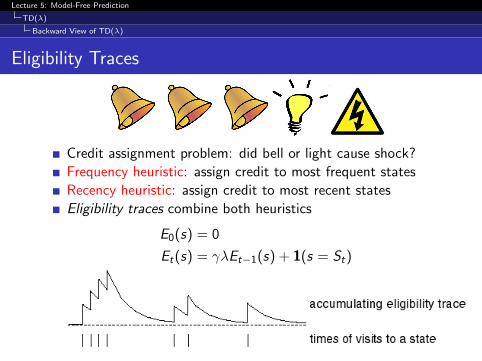
Eligibility Traces
Credit assignment problem: did bell or light cause shock?
Frequency heuristic: assign credit to most frequent states
Recency heuristic: assign credit to most recent states
Eligibility traces combine both heuristics
E0(s) = 0
Et(s) = γλEt−1(s) + 1(s = St)
Lecture 5: Model-Free Prediction
TD(λ)
Backward View of TD(λ)
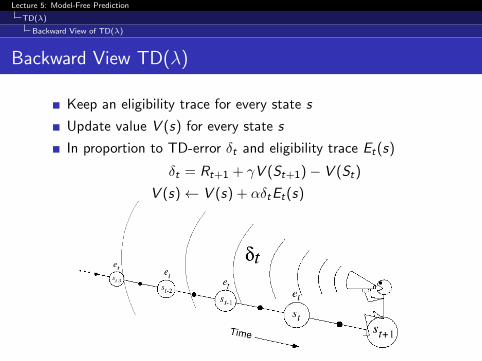
Backward View TD(λ)
Keep an eligibility trace for every state s
Update value V (s) for every state s
In proportion to TD-error δt and eligibility trace Et(s)
δt = Rt+1 + γV (St+1)− V (St)
V (s)← V (s) + αδtEt(s)
Lecture 5: Model-Free Prediction
TD(λ)
Backward View of TD(λ)
Backward-View TD(λ) Algorithm7.3. THE BACKWARD VIEW OF TD(�) 157
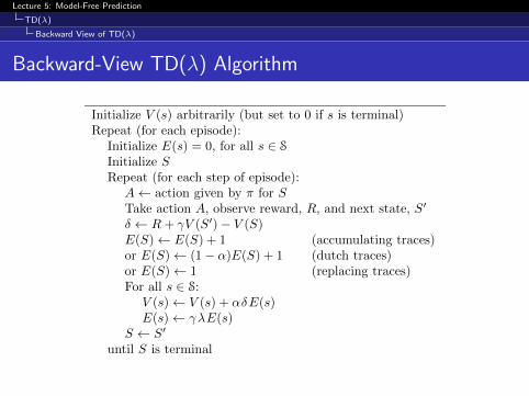
Initialize V (s) arbitrarily (but set to 0 if s is terminal)Repeat (for each episode):
Initialize E(s) = 0, for all s 2 S
Initialize SRepeat (for each step of episode):
A action given by ⇡ for STake action A, observe reward, R, and next state, S0
� R + �V (S0)� V (S)E(S) E(S) + 1 (accumulating traces)or E(S) (1� ↵)E(S) + 1 (dutch traces)or E(S) 1 (replacing traces)For all s 2 S:
V (s) V (s) + ↵�E(s)E(s) ��E(s)
S S0
until S is terminal
Figure 7.7: On-line tabular TD(�).
as suggested by the figure. We say that the earlier states are given less credit for theTD error.
If � = 1, then the credit given to earlier states falls only by � per step. Thisturns out to be just the right thing to do to achieve Monte Carlo behavior. Forexample, remember that the TD error, �t, includes an undiscounted term of Rt+1.In passing this back k steps it needs to be discounted, like any reward in a return,by �k, which is just what the falling eligibility trace achieves. If � = 1 and � = 1,then the eligibility traces do not decay at all with time. In this case the methodbehaves like a Monte Carlo method for an undiscounted, episodic task. If � = 1, thealgorithm is also known as TD(1).
!tet
et
et
et
Time
st
st+1
st-1
st-2
st-3
�t
St+1St
St-1St-2
St-3
xiv SUMMARY OF NOTATION
�t temporal-di�erence error at t (a random variable, even though not upper case)Et(s) eligibility trace for state s at tEt(s, a) eligibility trace for a state–action pairet eligibility trace vector at t
� discount-rate parameter� probability of random action in �-greedy policy�, � step-size parameters� decay-rate parameter for eligibility traces
Figure 7.8: The backward or mechanistic view. Each update depends on the current TDerror combined with eligibility traces of past events.
Lecture 5: Model-Free Prediction
TD(λ)
Relationship Between Forward and Backward TD
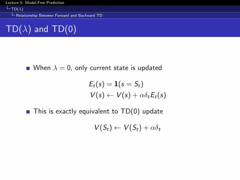
TD(λ) and TD(0)
When λ = 0, only current state is updated
Et(s) = 1(s = St)
V (s)← V (s) + αδtEt(s)
This is exactly equivalent to TD(0) update
V (St)← V (St) + αδt
Lecture 5: Model-Free Prediction
TD(λ)
Relationship Between Forward and Backward TD
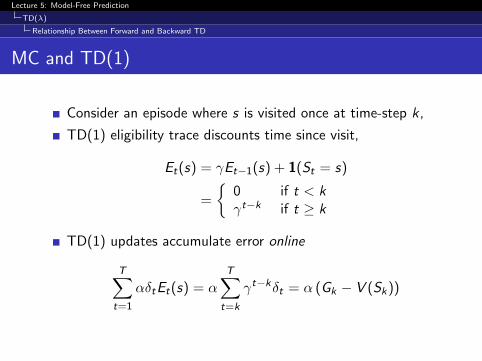
MC and TD(1)
Consider an episode where s is visited once at time-step k ,
TD(1) eligibility trace discounts time since visit,
Et(s) = γEt−1(s) + 1(St = s)
=
{0 if t < kγt−k if t ≥ k
TD(1) updates accumulate error online
T∑t=1
αδtEt(s) = αT∑
t=k
γt−kδt = α (Gk − V (Sk))
Lecture 5: Model-Free Prediction
TD(λ)
Relationship Between Forward and Backward TD
Telescoping in TD(1)
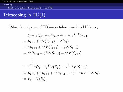
When λ = 1, sum of TD errors telescopes into MC error,
δt + γδt+1 + γ2δt+2 + ...+ γT−1δT−1
= Rt+1 + γV (St+1)− V (St)
+ γRt+2 + γ2V (St+2)− γV (St+1)
+ γ2Rt+3 + γ3V (St+3)− γ2V (St+2)
...
+ γT−1RT + γTV (ST )− γT−1V (ST−1)
= Rt+1 + γRt+2 + γ2Rt+3...+ γT−1RT − V (St)
= Gt − V (St)
Lecture 5: Model-Free Prediction
TD(λ)
Relationship Between Forward and Backward TD
TD(λ) and TD(1)
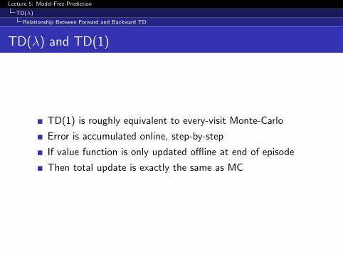
TD(1) is roughly equivalent to every-visit Monte-Carlo
Error is accumulated online, step-by-step
If value function is only updated offline at end of episode
Then total update is exactly the same as MC
Lecture 5: Model-Free Prediction
TD(λ)
Relationship Between Forward and Backward TD
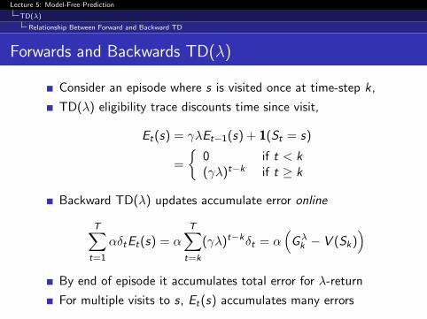
Forwards and Backwards TD(λ)
Consider an episode where s is visited once at time-step k ,
TD(λ) eligibility trace discounts time since visit,
Et(s) = γλEt−1(s) + 1(St = s)
=
{0 if t < k(γλ)t−k if t ≥ k
Backward TD(λ) updates accumulate error online
T∑t=1
αδtEt(s) = α
T∑t=k
(γλ)t−kδt = α(Gλk − V (Sk)
)By end of episode it accumulates total error for λ-return
For multiple visits to s, Et(s) accumulates many errors
Lecture 5: Model-Free Prediction
TD(λ)
Relationship Between Forward and Backward TD
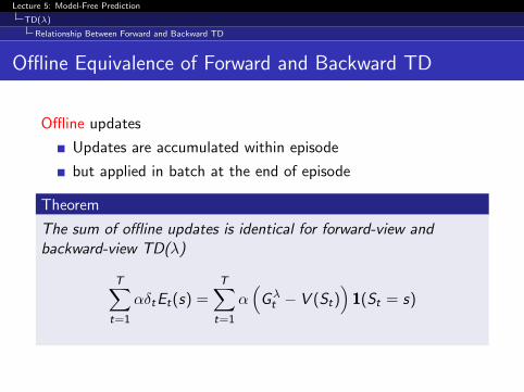
Offline Equivalence of Forward and Backward TD
Offline updates
Updates are accumulated within episode
but applied in batch at the end of episode
Theorem
The sum of offline updates is identical for forward-view andbackward-view TD(λ)
T∑t=1
αδtEt(s) =T∑t=1
α(Gλt − V (St)
)1(St = s)
Lecture 5: Model-Free Prediction
TD(λ)
Relationship Between Forward and Backward TD
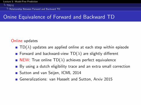
Onine Equivalence of Forward and Backward TD
Online updates
TD(λ) updates are applied online at each step within episode
Forward and backward-view TD(λ) are slightly different
NEW: True online TD(λ) achieves perfect equivalence
By using a dutch eligibility trace and an extra small correction
Sutton and van Seijen, ICML 2014
Generalizations: van Hasselt and Sutton, Arxiv 2015
Lecture 5: Model-Free Prediction
TD(λ)
Relationship Between Forward and Backward TD
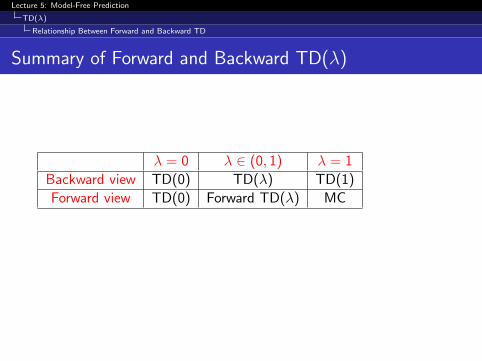
Summary of Forward and Backward TD(λ)
λ = 0 λ ∈ (0, 1) λ = 1
Backward view TD(0) TD(λ) TD(1)
Forward view TD(0) Forward TD(λ) MC