Lecture 5 Functional Form and Prediction

RS - Econometrics I - Lecture 5

1

1

Lecture 5Functional Form and Prediction

OLS Estimation - Assumptions

• CLM Assumptions

(A1) DGP: y = X + is correctly specified.

(A2) E[|X] = 0

(A3) Var[|X] = σ2 IT

(A4) X has full column rank –rank(X)=k–, where T ≥ k.

• In this lecture, again, we will look at assumption (A1). So far, we have restricted f(X,) to be a linear function: f(X,) = X .

• But, it turns out that in the framework of OLS estimation, we can be more flexible with f(X,).


2

• Linear in variables and parameters:

• Linear in parameters (intrinsic linear), nonlinear in variables:

Note: We get some nonlinear relation between y and X, but OLS still can be used.

4433221 XXXY

44332221 logXXXY

4433222 log,, XZXZXZ

4433221 ZZZY

7

Functional Form: Linearity in Parameters

X2

0 10 200

20

40


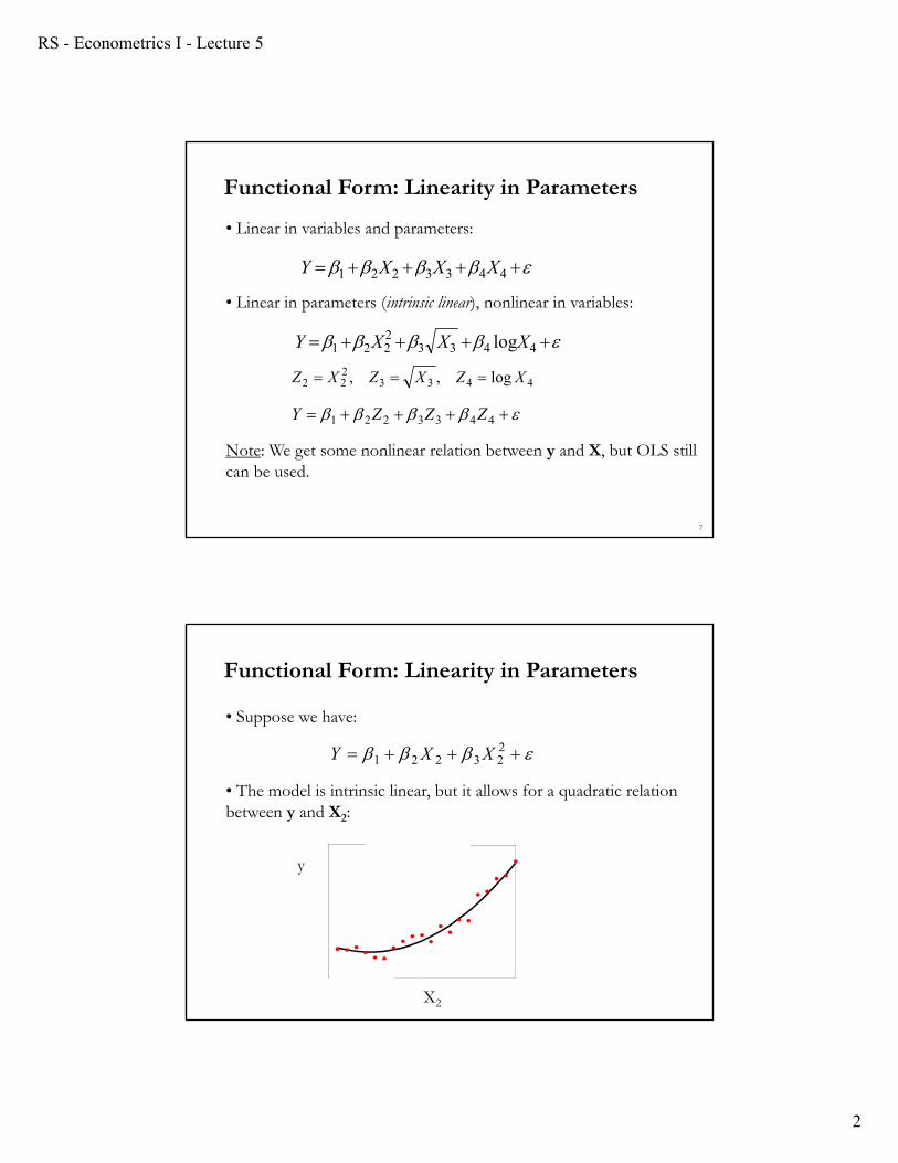
• Suppose we have:

• The model is intrinsic linear, but it allows for a quadratic relation between y and X2:

223221 XXY

y


3

[Matlab demo]

010

200

100

200

300

400

-10

0

10

20


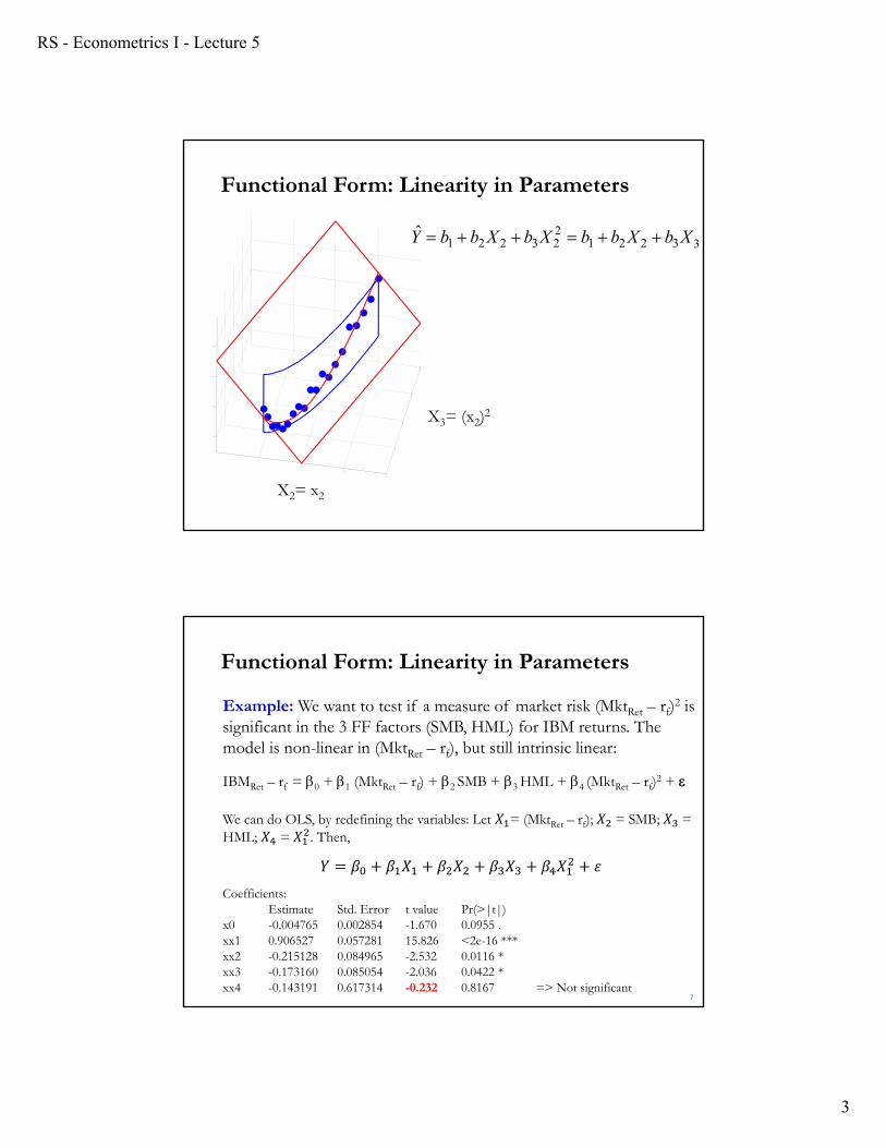
X2= x2

X3= (x2)2

33221223221

ˆ XbXbbXbXbbY

Example: We want to test if a measure of market risk (MktRet – rf)2 is significant in the 3 FF factors (SMB, HML) for IBM returns. The model is non-linear in (MktRet – rf), but still intrinsic linear:

IBMRet – rf = 0 + 1 (MktRet – rf) + 2 SMB + 3 HML + 4 (MktRet – rf)2 +

We can do OLS, by redefining the variables: Let 𝑋 = (MktRet – rf); 𝑋 = SMB; 𝑋 =HML; 𝑋 = 𝑋 . Then,

𝑌 𝛽 𝛽 𝑋 𝛽 𝑋 𝛽 𝑋 𝛽 𝑋 𝜀

Coefficients:Estimate Std. Error t value Pr(>|t|)

x0 -0.004765 0.002854 -1.670 0.0955 . xx1 0.906527 0.057281 15.826 <2e-16 ***xx2 -0.215128 0.084965 -2.532 0.0116 * xx3 -0.173160 0.085054 -2.036 0.0422 * xx4 -0.143191 0.617314 -0.232 0.8167 => Not significant

7



4

• We can approximate very complex non-linearities with polynomials of order k:

• Polynomial models are also useful as approximating functions to unknown nonlinear relationships. You can think of a polynomial model as the Taylor series expansion of the unknown function.

• Selecting the order of the polynomial –i.e., selecting k- is not trivial.

• k may be too large or too small.

k

k XXXXY 21323

223221 ...

7


• Nonlinear in parameters:

43233221 XXXY

This model is nonlinear in parameters since the coefficient of X4 is the product of the coefficients of X2 and X3.

• Some nonlinearities in parameters can be linearized by appropriate transformations, but not this one. This in not an intrinsic linear model.

7



5

25

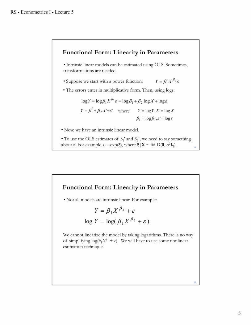
• Now, we have an intrinsic linear model.

• To use the OLS estimates of β1′ and β2′, we need to say something about ε. For example, =exp(ξ), where ξ|X ~ iid D(0, σ2IT).

21XY

logloglogloglog 2112 XXY

''' 2'

1 XY

log',log

log',log'

1'

1

XXYYwhere


• Intrinsic linear models can be estimated using OLS. Sometimes, transformations are needed.

• Suppose we start with a power function:

• The errors enter in multiplicative form. Then, using logs:

25


• Not all models are intrinsic linear. For example:

We cannot linearize the model by taking logarithms. There is no way of simplifying log(b1Xb + ε). We will have to use some nonlinear estimation technique.

21 XY

)log(log 21 XY


6

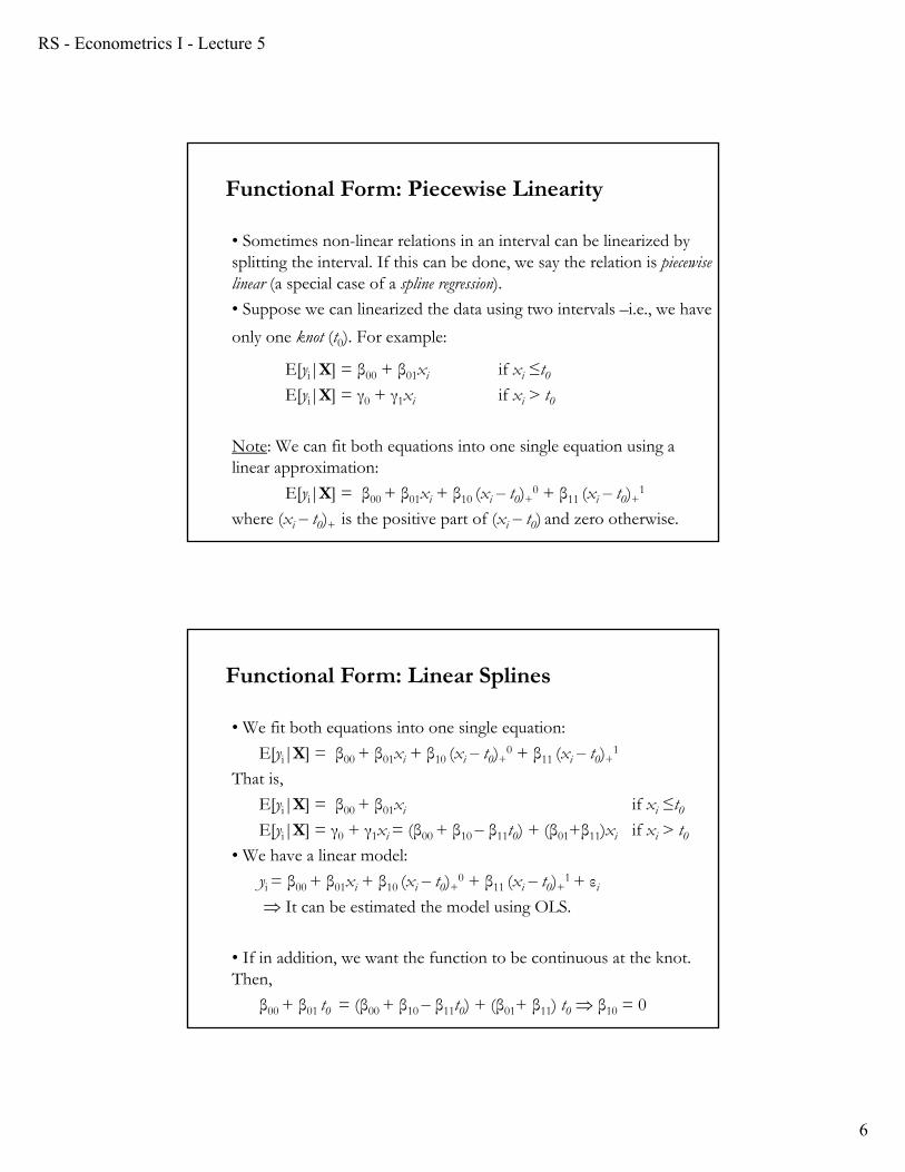
• Sometimes non-linear relations in an interval can be linearized by splitting the interval. If this can be done, we say the relation is piecewise linear (a special case of a spline regression).

• Suppose we can linearized the data using two intervals –i.e., we have

only one knot (t0). For example:

E[yi|X] = β00 + β01xi if xi ≤t0E[yi|X] = γ0 + γ1xi if xi > t0

Note: We can fit both equations into one single equation using a linear approximation:

E[yi|X] = β00 + β01xi + β10 (xi – t0)+0 + β11 (xi – t0)+

1

where (xi – t0)+ is the positive part of (xi – t0) and zero otherwise.

Functional Form: Piecewise Linearity

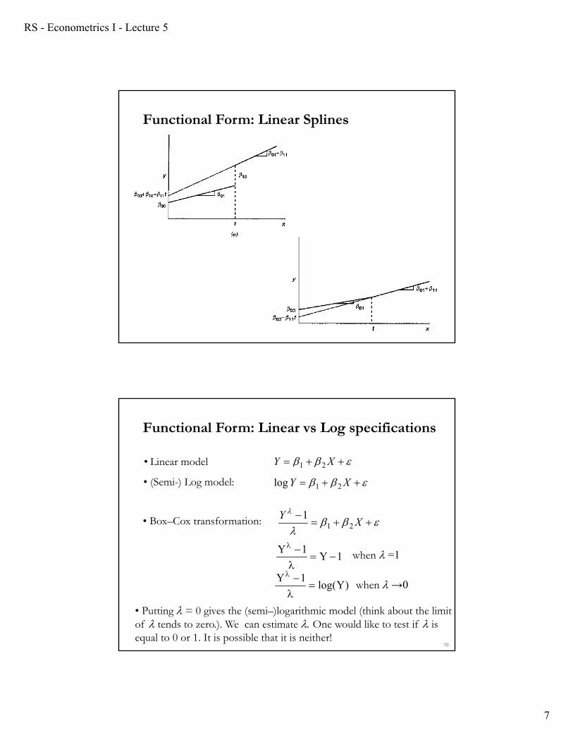
• We fit both equations into one single equation:

E[yi|X] = β00 + β01xi + β10 (xi – t0)+0 + β11 (xi – t0)+

1

That is,

E[yi|X] = β00 + β01xi if xi ≤t0E[yi|X] = γ0 + γ1xi = (β00 + β10 – β11t0) + (β01+β11)xi if xi > t0

• We have a linear model:

yi = β00 + β01xi + β10 (xi – t0)+0 + β11 (xi – t0)+

1 + εi

It can be estimated the model using OLS.

• If in addition, we want the function to be continuous at the knot. Then,

β00 + β01 t0 = (β00 + β10 – β11t0) + (β01+ β11) t0 β10 = 0

Functional Form: Linear Splines


7

Functional Form: Linear Splines

XY 21log

• Putting = 0 gives the (semi–)logarithmic model (think about the limit of tends to zero.). We can estimate One would like to test if is equal to 0 or 1. It is possible that it is neither!

X

Y21

1• Box–Cox transformation:

when =1

XY 21

10

Functional Form: Linear vs Log specifications

• Linear model

• (Semi-) Log model:

1Y1Y

)Ylog(1Y

when →0


8

• To test the specification of the functional form, Ramsey designed a simple test. We start with the fitted values:

ŷ = Xb.

Then, we add ŷ2 to the regression specification:

y = X + ŷ2 γ + ε

• If ŷ2 is added to the regression specification, it should pick up quadratic and interactive nonlinearity, if present, without necessarily being highly correlated with any of the X variables.

• We test H0 (linear functional form): γ = 0

H1 ( non linear functional form): γ ≠ 03

Functional Form: Ramsey’s RESET Test

• We test H0 (linear functional form): γ = 0

H1 ( non linear functional form): γ ≠ 0

t-test on the OLS estimator of γ.

• If the t-statistic for ŷ2 is significant evidence of nonlinearity.

• The RESET test is intended to detect nonlinearity, but not be specific about the most appropriate nonlinear model (no specific functional form is specified in H1).

3


James B. Ramsey, England


9

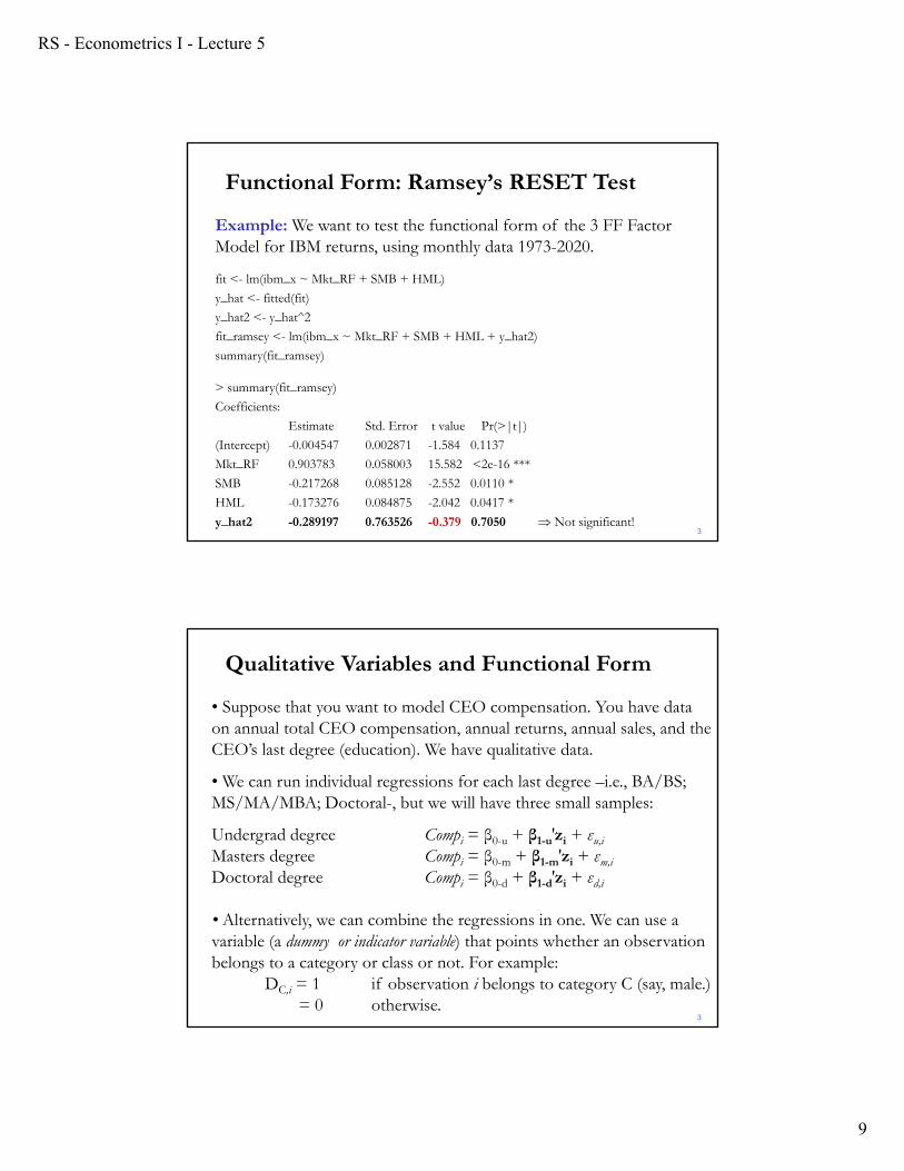
Example: We want to test the functional form of the 3 FF Factor Model for IBM returns, using monthly data 1973-2020.

fit <- lm(ibm_x ~ Mkt_RF + SMB + HML)

y_hat <- fitted(fit)

y_hat2 <- y_hat^2

fit_ramsey <- lm(ibm_x ~ Mkt_RF + SMB + HML + y_hat2)

summary(fit_ramsey)

> summary(fit_ramsey)

Coefficients:

Estimate Std. Error t value Pr(>|t|)

(Intercept) -0.004547 0.002871 -1.584 0.1137

Mkt_RF 0.903783 0.058003 15.582 <2e-16 ***

SMB -0.217268 0.085128 -2.552 0.0110 *

HML -0.173276 0.084875 -2.042 0.0417 *

y_hat2 -0.289197 0.763526 -0.379 0.7050 Not significant!3


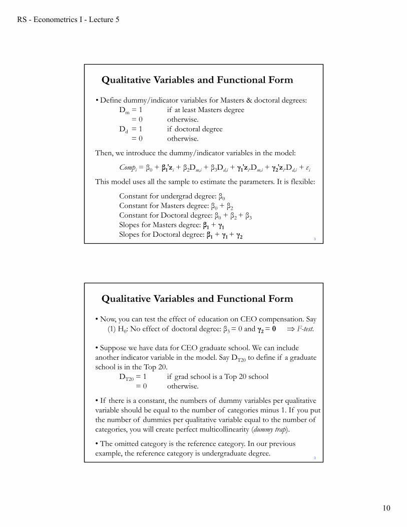
• Suppose that you want to model CEO compensation. You have data on annual total CEO compensation, annual returns, annual sales, and the CEO’s last degree (education). We have qualitative data.

• We can run individual regressions for each last degree –i.e., BA/BS; MS/MA/MBA; Doctoral-, but we will have three small samples:

Undergrad degree Compi = β0-u + β1-u′zi + εu,i

Masters degree Compi = β0-m + β1-m′zi + εm,i

Doctoral degree Compi = β0-d + β1-d′zi + εd,i

• Alternatively, we can combine the regressions in one. We can use a variable (a dummy or indicator variable) that points whether an observation belongs to a category or class or not. For example:

DC,i = 1 if observation i belongs to category C (say, male.)= 0 otherwise.

3

Qualitative Variables and Functional Form


10

• Define dummy/indicator variables for Masters & doctoral degrees: Dm = 1 if at least Masters degree

= 0 otherwise.Dd = 1 if doctoral degree

= 0 otherwise.

Then, we introduce the dummy/indicator variables in the model:

Compi = β0 + β1′zi + β2Dm,i + β3Dd,i + γ1′zi.Dm,i + γ2′zi.Dd,i + εi

This model uses all the sample to estimate the parameters. It is flexible:

Constant for undergrad degree: β0

Constant for Masters degree: β0 + β2

Constant for Doctoral degree: β0 + β2 + β3

Slopes for Masters degree: β1 + γ1

Slopes for Doctoral degree: β1 + γ1 + γ2 3


• Now, you can test the effect of education on CEO compensation. Say (1) H0: No effect of doctoral degree: β3 = 0 and γ2 = 0 F-test.

• Suppose we have data for CEO graduate school. We can include another indicator variable in the model. Say DT20 to define if a graduate school is in the Top 20.

DT20 = 1 if grad school is a Top 20 school= 0 otherwise.

• If there is a constant, the numbers of dummy variables per qualitative variable should be equal to the number of categories minus 1. If you put the number of dummies per qualitative variable equal to the number of categories, you will create perfect multicollinearity (dummy trap).

• The omitted category is the reference category. In our previous example, the reference category is undergraduate degree.

3



11

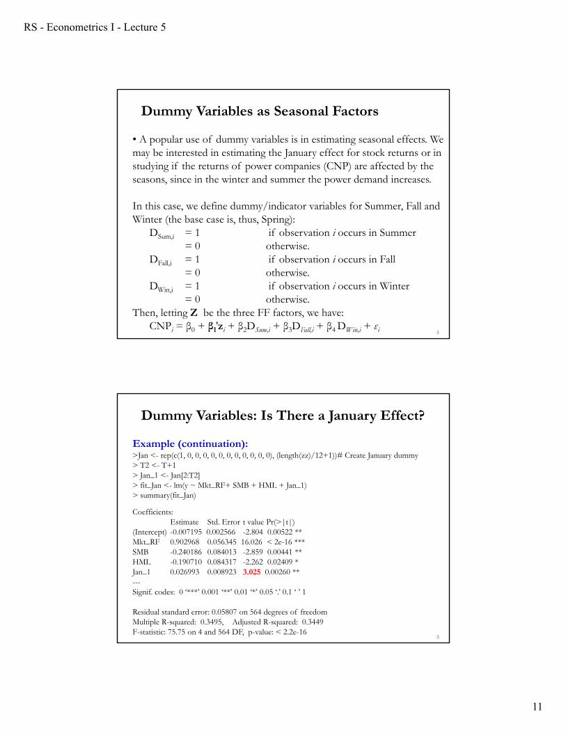
• A popular use of dummy variables is in estimating seasonal effects. We may be interested in estimating the January effect for stock returns or in studying if the returns of power companies (CNP) are affected by the seasons, since in the winter and summer the power demand increases.

In this case, we define dummy/indicator variables for Summer, Fall and Winter (the base case is, thus, Spring):

DSum,i = 1 if observation i occurs in Summer= 0 otherwise.

DFall,i = 1 if observation i occurs in Fall = 0 otherwise.

DWin,i = 1 if observation i occurs in Winter = 0 otherwise.

Then, letting Z be the three FF factors, we have:CNPi = β0 + β1′zi + β2DSum,i + β3DFall,i + β4 DWin,i + εi 3

Dummy Variables as Seasonal Factors

Example (continuation):>Jan <- rep(c(1, 0, 0, 0, 0, 0, 0, 0, 0, 0, 0, 0), (length(zz)/12+1))# Create January dummy> T2 <- T+1> Jan_1 <- Jan[2:T2]> fit_Jan <- lm(y ~ Mkt_RF+ SMB + HML + Jan_1)> summary(fit_Jan)


(Intercept) -0.007195 0.002566 -2.804 0.00522 ** Mkt_RF 0.902968 0.056345 16.026 < 2e-16 ***SMB -0.240186 0.084013 -2.859 0.00441 ** HML -0.190710 0.084317 -2.262 0.02409 * Jan_1 0.026993 0.008923 3.025 0.00260 ** ---Signif. codes: 0 ‘***’ 0.001 ‘**’ 0.01 ‘*’ 0.05 ‘.’ 0.1 ‘ ’ 1

Residual standard error: 0.05807 on 564 degrees of freedomMultiple R-squared: 0.3495, Adjusted R-squared: 0.3449 F-statistic: 75.75 on 4 and 564 DF, p-value: < 2.2e-16

3

Dummy Variables: Is There a January Effect?


12

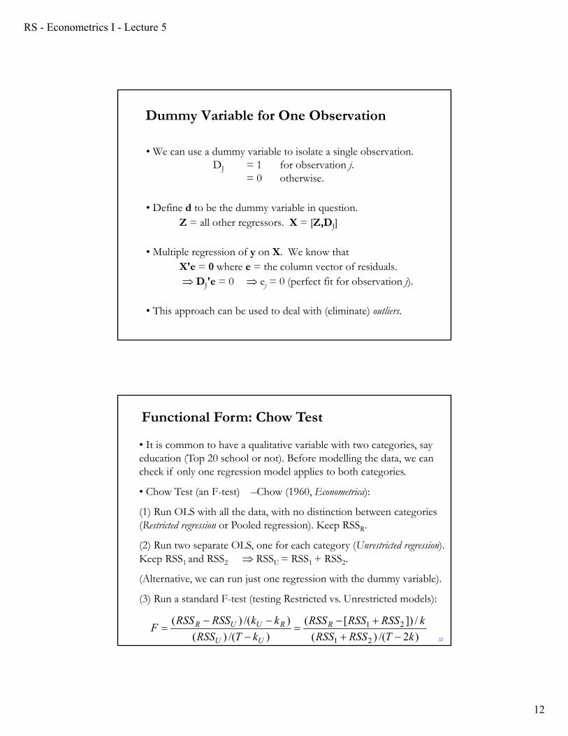
Dummy Variable for One Observation

• We can use a dummy variable to isolate a single observation. DJ = 1 for observation j.

= 0 otherwise.

• Define d to be the dummy variable in question. Z = all other regressors. X = [Z,DJ]

• Multiple regression of y on X. We know that X'e = 0 where e = the column vector of residuals. DJ'e = 0 ej = 0 (perfect fit for observation j).

• This approach can be used to deal with (eliminate) outliers.

32

Functional Form: Chow Test

• It is common to have a qualitative variable with two categories, say education (Top 20 school or not). Before modelling the data, we can check if only one regression model applies to both categories.

• Chow Test (an F-test) –Chow (1960, Econometrica):

(1) Run OLS with all the data, with no distinction between categories (Restricted regression or Pooled regression). Keep RSSR.

(2) Run two separate OLS, one for each category (Unrestricted regression). Keep RSS1 and RSS2 RSSU = RSS1 + RSS2.

(Alternative, we can run just one regression with the dummy variable).

(3) Run a standard F-test (testing Restricted vs. Unrestricted models):

)2/()(

/])[(

)/()(

)/()(

21

21

kTRSSRSS

kRSSRSSRSS

kTRSS

kkRSSRSSF R

UU

RUUR


13

32

Functional Form: Chow Test

• A Wald Test can also be used to compare the coefficient estimates, in the two samples (regimes 1 & 2), with T1 and T2 observations, respectively:

• This test is a bit more flexible, since it is easy to allow for different formulations for Var[ β β ]. (In econometrics, violations of (A3) are common, for example, different variances in regimes 1 & 2.)

𝑊 𝑇 β β ′𝑉𝑎𝑟 β β β β

Gregory C. Chow (1929, USA)

Chow Test: Males or Females visit doctors more?

• Taken from Greene

German Health Care Usage Data, 7,293 Individuals, Varying Numbers of PeriodsVariables in the file areData downloaded from Journal of Applied Econometrics Archive. This is an unbalanced panel with 7,293 individuals. There are altogether 27,326 observations. The number of observations ranges from 1 to 7 per family. (Frequencies are: 1=1525, 2=2158, 3=825, 4=926, 5=1051, 6=1000, 7=987). The dependent variable of interest is

DOCVIS = number of visits to the doctor in the observation period

HHNINC = household nominal monthly net income in German marks / 10000.(4 observations with income=0 were dropped)

HHKIDS = children under age 16 in the household = 1; otherwise = 0EDUC = years of schooling AGE = age in yearsMARRIED= marital status (1 = if married)WHITEC = 1 if has “white collar” job


14

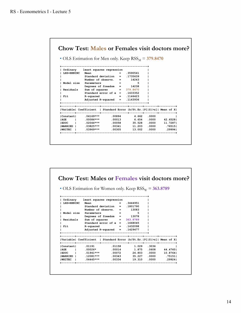
+----------------------------------------------------+| Ordinary least squares regression || LHS=HHNINC Mean = .3590541 || Standard deviation = .1735639 || Number of observs. = 14243 || Model size Parameters = 5 || Degrees of freedom = 14238 || Residuals Sum of squares = 379.8470 || Standard error of e = .1633352 || Fit R-squared = .1146423 || Adjusted R-squared = .1143936 |+----------------------------------------------------++--------+--------------+----------------+--------+--------+----------+|Variable| Coefficient | Standard Error |b/St.Er.|P[|Z|>z]| Mean of X|+--------+--------------+----------------+--------+--------+----------+|Constant| .04169*** .00894 4.662 .0000 ||AGE | .00086*** .00013 6.654 .0000 42.6528||EDUC | .02044*** .00058 35.528 .0000 11.7287||MARRIED | .03825*** .00341 11.203 .0000 .76515||WHITEC | .03969*** .00305 13.002 .0000 .29994|+--------+------------------------------------------------------------+


• OLS Estimation for Men only. Keep RSSM = 379.8470

+----------------------------------------------------+| Ordinary least squares regression || LHS=HHNINC Mean = .3444951 || Standard deviation = .1801790 || Number of observs. = 13083 || Model size Parameters = 5 || Degrees of freedom = 13078 || Residuals Sum of squares = 363.8789 || Standard error of e = .1668045 || Fit R-squared = .1432098 || Adjusted R-squared = .1429477 |+----------------------------------------------------++--------+--------------+----------------+--------+--------+----------+|Variable| Coefficient | Standard Error |b/St.Er.|P[|Z|>z]| Mean of X|+--------+--------------+----------------+--------+--------+----------+|Constant| .01191 .01158 1.029 .3036 ||AGE | .00026* .00014 1.875 .0608 44.4760||EDUC | .01941*** .00072 26.803 .0000 10.8764||MARRIED | .12081*** .00343 35.227 .0000 .75151||WHITEC | .06445*** .00334 19.310 .0000 .29924|+--------+------------------------------------------------------------+


• OLS Estimation for Women only. Keep RSSW = 363.8789


15

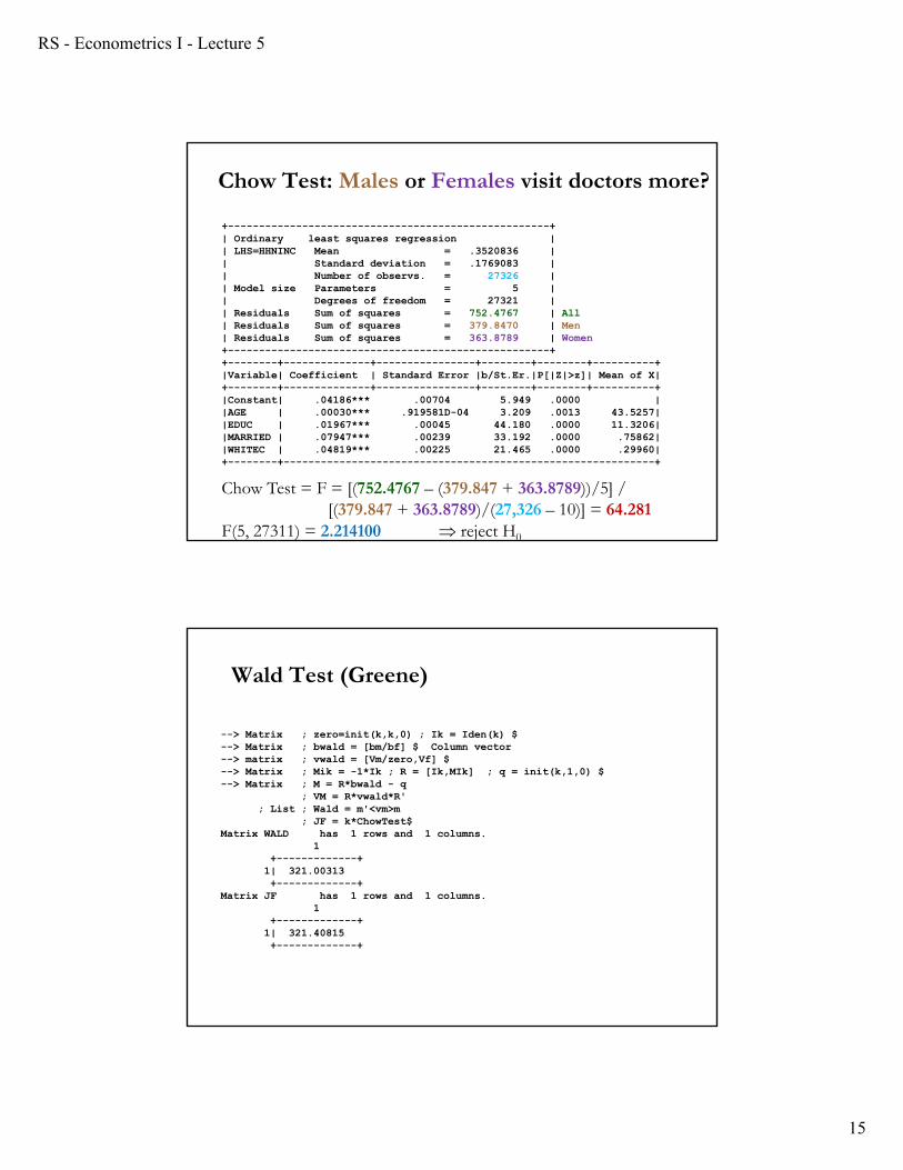
+----------------------------------------------------+| Ordinary least squares regression || LHS=HHNINC Mean = .3520836 || Standard deviation = .1769083 || Number of observs. = 27326 || Model size Parameters = 5 || Degrees of freedom = 27321 || Residuals Sum of squares = 752.4767 | All| Residuals Sum of squares = 379.8470 | Men| Residuals Sum of squares = 363.8789 | Women+----------------------------------------------------++--------+--------------+----------------+--------+--------+----------+|Variable| Coefficient | Standard Error |b/St.Er.|P[|Z|>z]| Mean of X|+--------+--------------+----------------+--------+--------+----------+|Constant| .04186*** .00704 5.949 .0000 ||AGE | .00030*** .919581D-04 3.209 .0013 43.5257||EDUC | .01967*** .00045 44.180 .0000 11.3206||MARRIED | .07947*** .00239 33.192 .0000 .75862||WHITEC | .04819*** .00225 21.465 .0000 .29960|+--------+------------------------------------------------------------+

Chow Test = F = [(752.4767 – (379.847 + 363.8789))/5] / [(379.847 + 363.8789)/(27,326 – 10)] = 64.281

F(5, 27311) = 2.214100 reject H0


Wald Test (Greene)

--> Matrix ; zero=init(k,k,0) ; Ik = Iden(k) $--> Matrix ; bwald = [bm/bf] $ Column vector--> matrix ; vwald = [Vm/zero,Vf] $--> Matrix ; Mik = -1*Ik ; R = [Ik,MIk] ; q = init(k,1,0) $--> Matrix ; M = R*bwald - q

; VM = R*vwald*R'; List ; Wald = m'<vm>m

; JF = k*ChowTest$Matrix WALD has 1 rows and 1 columns.

1+-------------+1| 321.00313+-------------+

Matrix JF has 1 rows and 1 columns.1

+-------------+1| 321.40815+-------------+


16

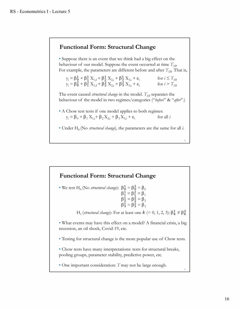
• Suppose there is an event that we think had a big effect on the behaviour of our model. Suppose the event occurred at time TSB.For example, the parameters are different before and after TSB. That is,

yi = + X1,I + X2,i + X3,i + i for i ≤ TSB

yi = + X1,I + X2,i + X3,i + i for i > TSB

The event caused structural change in the model. TSB separates the behaviour of the model in two regimes/categories (“before” & “after”.)

• A Chow test tests if one model applies to both regimes:yi = 0 + 1 X1,i+ 2 X2,i + 3 X3,i + i for all i

• Under H0 (No structural change), the parameters are the same for all i.

3

Functional Form: Structural Change

• We test H0 (No structural change): = = 0

= = 1

= = 2

= = 3

H1 (structural change): For at least one 𝑘 (= 0, 1, 2, 3): ≠

• What events may have this effect on a model? A financial crisis, a big recession, an oil shock, Covid-19, etc.

• Testing for structural change is the more popular use of Chow tests.

• Chow tests have many interpretations: tests for structural breaks, pooling groups, parameter stability, predictive power, etc.

• One important consideration: T may not be large enough. 3



17

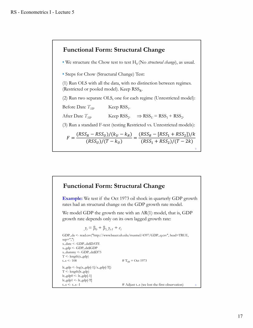
• We structure the Chow test to test H0 (No structural change), as usual.

• Steps for Chow (Structural Change) Test:

(1) Run OLS with all the data, with no distinction between regimes. (Restricted or pooled model). Keep RSSR.

(2) Run two separate OLS, one for each regime (Unrestricted model):

Before Date TSB. Keep RSS1.

After Date TSB. Keep RSS2. RSSU = RSS1 + RSS2.

(3) Run a standard F-test (testing Restricted vs. Unrestricted models):

𝐹𝑅𝑆𝑆 𝑅𝑆𝑆 / 𝑘 𝑘

𝑅𝑆𝑆 / 𝑇 𝑘𝑅𝑆𝑆 𝑅𝑆𝑆 𝑅𝑆𝑆 /𝑘𝑅𝑆𝑆 𝑅𝑆𝑆 / 𝑇 2𝑘

3


Example: We test if the Oct 1973 oil shock in quarterly GDP growth rates had an structural change on the GDP growth rate model.

We model GDP the growth rate with an AR(1) model, that is, GDP growth rate depends only on its own lagged growth rate:

yt = β0 + β1 yt-1 + εiGDP_da <- read.csv("http://www.bauer.uh.edu/rsusmel/4397/GDP_q.csv", head=TRUE, sep=",")x_date <- GDP_da$DATEx_gdp <- GDP_da$GDPx_dummy <- GDP_da$D73T <- length(x_gdp)t_s <- 108 # TSB = Oct 1973

lr_gdp <- log(x_gdp[-1]/x_gdp[-T])T <- length(lr_gdp)lr_gdp0 <- lr_gdp[-1]lr_gdp1 <- lr_gdp[-T]t_s <- t_s -1 # Adjust t_s (we lost the first observation) 3



18

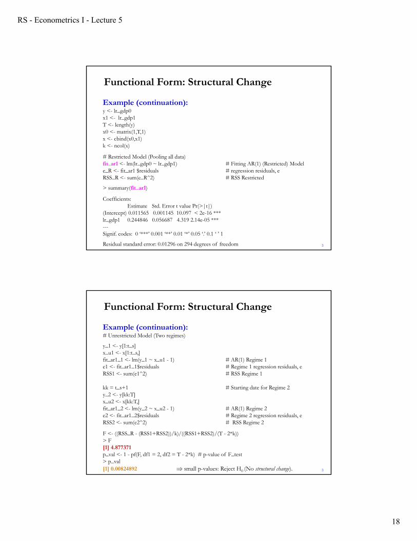
Example (continuation):y <- lr_gdp0 x1 <- lr_gdp1T <- length(y)x0 <- matrix(1,T,1)x <- cbind(x0,x1)k <- ncol(x)

# Restricted Model (Pooling all data)fit_ar1 <- lm(lr_gdp0 ~ lr_gdp1) # Fitting AR(1) (Restricted) Modele_R <- fit_ar1 $residuals # regression residuals, eRSS_R <- sum(e_R^2) # RSS Restricted

> summary(fit_ar1)


(Intercept) 0.011565 0.001145 10.097 < 2e-16 ***lr_gdp1 0.244846 0.056687 4.319 2.14e-05 ***---Signif. codes: 0 ‘***’ 0.001 ‘**’ 0.01 ‘*’ 0.05 ‘.’ 0.1 ‘ ’ 1

Residual standard error: 0.01296 on 294 degrees of freedom 3


Example (continuation):# Unrestricted Model (Two regimes)

y_1 <- y[1:t_s]x_u1 <- x[1:t_s,]fit_ar1_1 <- lm(y_1 ~ x_u1 - 1) # AR(1) Regime 1e1 <- fit_ar1_1$residuals # Regime 1 regression residuals, eRSS1 <- sum(e1^2) # RSS Regime 1

kk = t_s+1 # Starting date for Regime 2y_2 <- y[kk:T]x_u2 <- x[kk:T,]fit_ar1_2 <- lm(y_2 ~ x_u2 - 1) # AR(1) Regime 2e2 <- fit_ar1_2$residuals # Regime 2 regression residuals, eRSS2 <- sum(e2^2) # RSS Regime 2

F <- ((RSS_R - (RSS1+RSS2))/k)/((RSS1+RSS2)/(T - 2*k))> F[1] 4.877371p_val <- 1 - pf(F, df1 = 2, df2 = T - 2*k) # p-value of F_test> p_val[1] 0.00824892 small p-values: Reject H0 (No structural change). 3



19

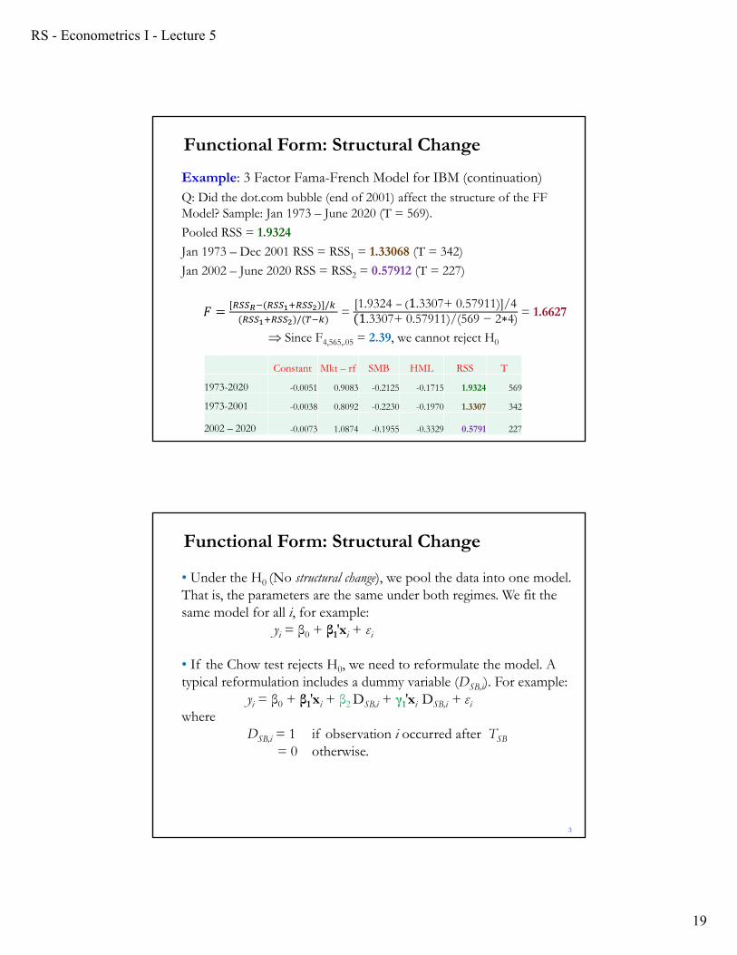
Example: 3 Factor Fama-French Model for IBM (continuation)Q: Did the dot.com bubble (end of 2001) affect the structure of the FF Model? Sample: Jan 1973 – June 2020 (T = 569).

Pooled RSS = 1.9324

Jan 1973 – Dec 2001 RSS = RSS1 = 1.33068 (T = 342)

Jan 2002 – June 2020 RSS = RSS2 = 0.57912 (T = 227)

𝐹 /

/=

[1.9324 1.3307+ 0.57911)]/41.3307+ 0.57911)/(569 − 2∗4) = 1.6627

Since F4,565,.05 = 2.39, we cannot reject H0

Constant Mkt – rf SMB HML RSS T

1973-2020 -0.0051 0.9083 -0.2125 -0.1715 1.9324 569

1973-2001 -0.0038 0.8092 -0.2230 -0.1970 1.3307 342

2002 – 2020 -0.0073 1.0874 -0.1955 -0.3329 0.5791 227


• Under the H0 (No structural change), we pool the data into one model. That is, the parameters are the same under both regimes. We fit the same model for all i, for example:

yi = β0 + β1′xi + εi

• If the Chow test rejects H0, we need to reformulate the model. A typical reformulation includes a dummy variable (DSB,i). For example:

yi = β0 + β1′xi + β2 DSB,i + γ1′xi DSB,i + εiwhere

DSB,i = 1 if observation i occurred after TSB

= 0 otherwise.

3



20

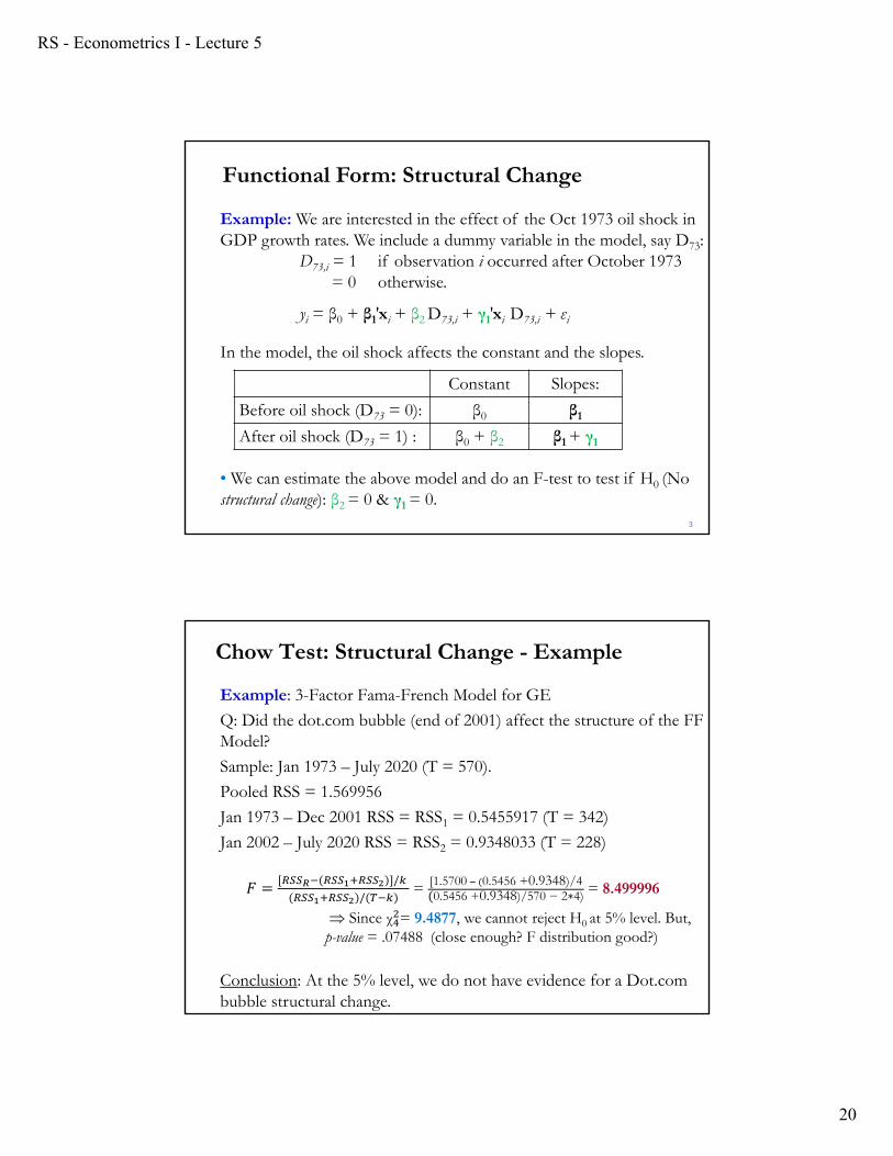
Example: We are interested in the effect of the Oct 1973 oil shock in GDP growth rates. We include a dummy variable in the model, say D73:

D73,i = 1 if observation i occurred after October 1973= 0 otherwise.

yi = β0 + β1′xi + β2 D73,i + γ1′xi D73,i + εi

In the model, the oil shock affects the constant and the slopes.

• We can estimate the above model and do an F-test to test if H0 (No structural change): β2 = 0 & γ1 = 0.

3

Constant Slopes:

Before oil shock (D73 = 0): β0 β1

After oil shock (D73 = 1) : β0 + β2 β1 + γ1


Chow Test: Structural Change - Example

Example: 3-Factor Fama-French Model for GE

Q: Did the dot.com bubble (end of 2001) affect the structure of the FF Model?

Sample: Jan 1973 – July 2020 (T = 570).

Pooled RSS = 1.569956

Jan 1973 – Dec 2001 RSS = RSS1 = 0.5455917 (T = 342)

Jan 2002 – July 2020 RSS = RSS2 = 0.9348033 (T = 228)

𝐹 /

/= [1.5700 0.5456 +0.9348)/4

0.5456 +0.9348)/570 − 2∗4) = 8.499996

Since χ = 9.4877, we cannot reject H0 at 5% level. But, p-value = .07488 (close enough? F distribution good?)

Conclusion: At the 5% level, we do not have evidence for a Dot.com bubble structural change.


21

• But, we can try different breaking points, starting at T=85:

Chow Test: Structural Change - Example

Note: Recall that the Chow test is an F-test, we are testing a joint hypothesis, all coefficients are subject to structural change.

Example (continuation): Now, we check the effect of the dot.com bubble (create dummy) on the constant using a t-test:T <- length(ge_x)

x_break <- 342

dot_0 <- rep(0, x_break) # 0 up to Dec 2001

dot_1 <- rep(1, T - x_break) # 1 after Dec 2001

dot <- c(dot_0,dot_1) # Doc.com dummy

fit_ge_dot <- lm(ge_x ~ Mkt_RF + SMB + HML + dot)

> summary(fit_ge_dot)

Coefficients:


(Intercept) -0.003273 0.002877 -1.138 0.25566

Mkt_RF 1.226412 0.050868 24.110 < 2e-16 ***

SMB -0.308411 0.075433 -4.089 4.97e-05 ***

HML 0.341709 0.075755 4.511 7.86e-06 ***

dot -0.013052 0.004502 -2.899 0.00388 ** significant effect on constant.

Chow Test: Structural Change in Constant


22

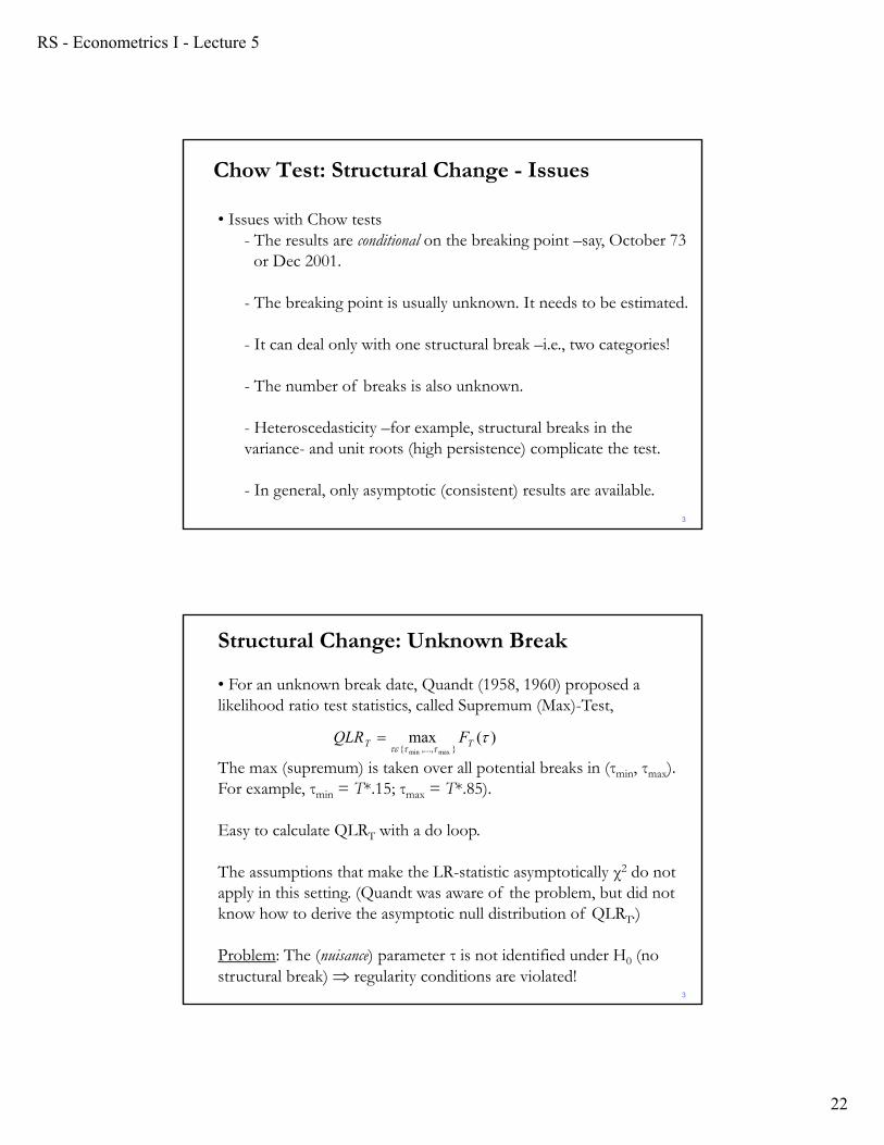
• Issues with Chow tests- The results are conditional on the breaking point –say, October 73

or Dec 2001.

- The breaking point is usually unknown. It needs to be estimated.

- It can deal only with one structural break –i.e., two categories!

- The number of breaks is also unknown.

- Heteroscedasticity –for example, structural breaks in the variance- and unit roots (high persistence) complicate the test.

- In general, only asymptotic (consistent) results are available.

3

Chow Test: Structural Change - Issues

• For an unknown break date, Quandt (1958, 1960) proposed a likelihood ratio test statistics, called Supremum (Max)-Test,

The max (supremum) is taken over all potential breaks in (τmin, τmax). For example, τmin = T*.15; τmax = T*.85).

Easy to calculate QLRT with a do loop.

The assumptions that make the LR-statistic asymptotically χ2 do not apply in this setting. (Quandt was aware of the problem, but did not know how to derive the asymptotic null distribution of QLRT.)

Problem: The (nuisance) parameter τ is not identified under H0 (no structural break) regularity conditions are violated!

3

)(max},...,{ maxmin

TT FQLR

Structural Change: Unknown Break


23

• Andrews (1993) showed that under appropriate regularity conditions, the QLR statistic, also referred to as a SupLR statistic, has a nonstandard limiting distribution:

where 0< rmin< rmax<1 and Bk(.) is a “Brownian Bridge” process defined on [0,1]. Percentiles of this distribution as functions of rmax, rmin and kare tabulated in Andrews (1993). (Critical values much larger than χ2.)

Note: A Brownian bridge is a continuous-time stochastic process B(t) whose probability distribution is the conditional probability distribution of a Wiener process W(t) given the condition that B(0) = B(1) = 0. The increments in a Brownian bridge are not independent.Example: B(t) = W(t) – t W(1) is a Brownian Bridge.

3

))1(

)()'((sup ],[ maxmin rr

rBrBQLR kk

rrrd

T

Structural Change: Unknown Break

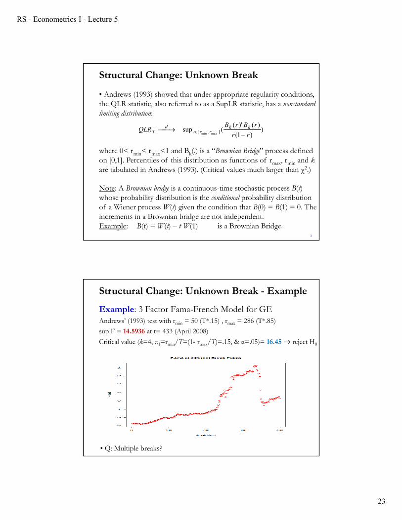
Example: 3 Factor Fama-French Model for GEAndrews’ (1993) test with rmin = 50 (T*.15) , rmax = 286 (T*.85)

sup F = 14.5936 at t= 433 (April 2008)

Critical value (k=4, π1=rmin/T=(1- rmax/T)=.15, & α=.05)= 16.45 reject H0

• Q: Multiple breaks?

Structural Change: Unknown Break - Example


24

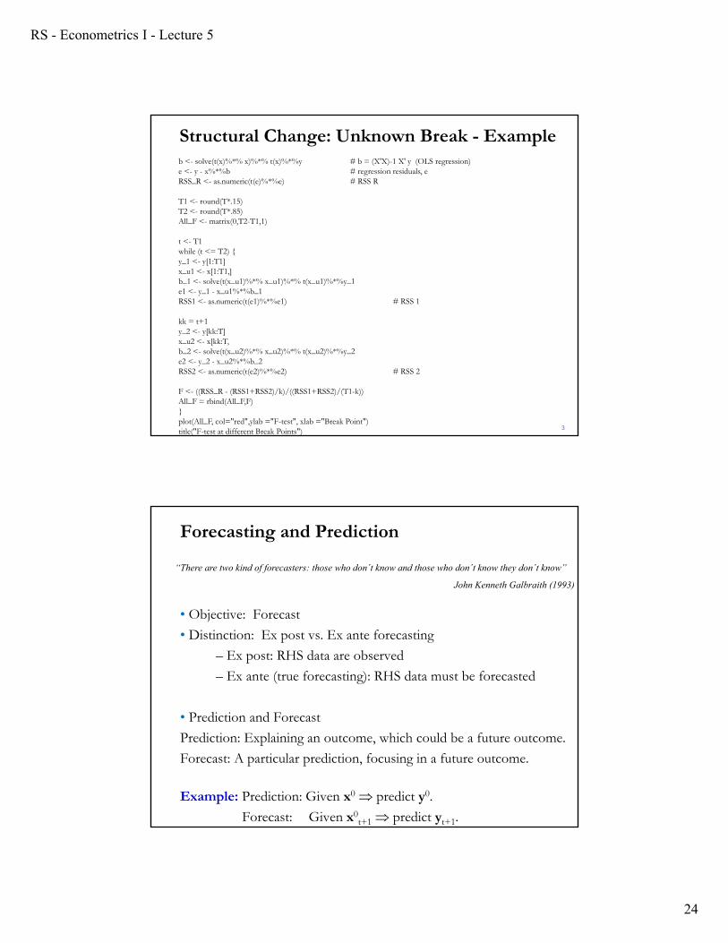
b <- solve(t(x)%*% x)%*% t(x)%*%y # b = (X'X)-1 X' y (OLS regression)e <- y - x%*%b # regression residuals, eRSS_R <- as.numeric(t(e)%*%e) # RSS R

T1 <- round(T*.15)T2 <- round(T*.85)All_F <- matrix(0,T2-T1,1)

t <- T1while (t <= T2) {y_1 <- y[1:T1]x_u1 <- x[1:T1,]b_1 <- solve(t(x_u1)%*% x_u1)%*% t(x_u1)%*%y_1 e1 <- y_1 - x_u1%*%b_1RSS1 <- as.numeric(t(e1)%*%e1) # RSS 1

kk = t+1y_2 <- y[kk:T]x_u2 <- x[kk:T,b_2 <- solve(t(x_u2)%*% x_u2)%*% t(x_u2)%*%y_2 e2 <- y_2 - x_u2%*%b_2RSS2 <- as.numeric(t(e2)%*%e2) # RSS 2

F <- ((RSS_R - (RSS1+RSS2)/k)/((RSS1+RSS2)/(T1-k))All_F = rbind(All_F,F)}plot(All_F, col="red",ylab ="F-test", xlab ="Break Point")title("F-test at different Break Points") 3

Structural Change: Unknown Break - Example

Forecasting and Prediction

• Objective: Forecast

• Distinction: Ex post vs. Ex ante forecasting

– Ex post: RHS data are observed

– Ex ante (true forecasting): RHS data must be forecasted

• Prediction and Forecast

Prediction: Explaining an outcome, which could be a future outcome.

Forecast: A particular prediction, focusing in a future outcome.

Example: Prediction: Given x0 predict y0.

Forecast: Given x0t+1 predict yt+1.

“There are two kind of forecasters: those who don´t know and those who don´t know they don´t know”

John Kenneth Galbraith (1993)


25


• Two types of predictions:

- In sample (prediction): The expected value of y (in-sample), given the estimates of the parameters.

- Out of sample (forecasting): The value of a future y that is not observed by the sample.

Notation: - Prediction for T made at T: 𝑌 .- Forecast for T+l made at T: 𝑌 , 𝑌 | , 𝑌 𝑙 .

where T is the forecast origin and l is the forecast horizon. Then,

𝑌 𝑙 : l-step ahead forecast = Forecasted value YT+l at time T.


• Any prediction or forecast needs an information set, IT. This includes data, models and/or assumptions available at time T. The predictions and forecasts will be conditional on IT.

For example, in-sample , IT = {x0} to predict y0. Or in a time series context, IT = {x0

T-1, x0T-2, ..., x0

T-q} to predict yt+l.

• Then, the forecast is just the conditional expectation of YT+l, giventhe observed sample:

𝑌 𝐸 𝑌 |𝑋 ,𝑋 , … ,𝑋

Example: If 𝑋 𝑌 , then, the one-step ahead forecast is:

𝑌 𝐸 𝑌 |𝑌 ,𝑌 , … ,𝑌


26


• Keep in mind that the forecasts are a random variable. Technically speaking, they can be fully characterized by a pdf.

• In general, it is difficult to get the pdf for the forecast. In practice, we get a point estimate (the forecast) and a C.I.


• Prediction vs. model validation.

– Within sample prediction: Using the whole sample (T observations), we predict y as usual, with 𝑦.

– Hold out sample: We estimate the model only using a part of the sample (say, up to time T1). The rest of the sample (T-T1 observations) are used to check the predictive power of the model –i.e., the accuracy of predictions, by comparing y0

with actual y).

Model validation refers to establishing the statistical adequacy of the assumptions behind the model –i.e., (A1)-(A5) in this lecture. Predictive power can be used to do model validation.


27

Forecasting

0.0000

0.2000

0.4000

0.6000

0.8000

1.0000

1.2000

Jan-

99

Jul-9

9

Jan-

00

Jul-0

0

Jan-

01

Jul-0

1

Jan-

02

Jul-0

2

Jan-

03

Jul-0

3

Jan-

04

Jul-0

4

Jan-

05

Jul-0

5

Jan-

06

Jul-0

6

Jan-

07

Jul-0

7

Jan-

08

Jul-0

8

Jan-

09

Jul-0

9

Jan-

10

Jul-1

0

AUD/USD

Estimation Period

Out-of-Sample Forecasts

Validation Forecasts

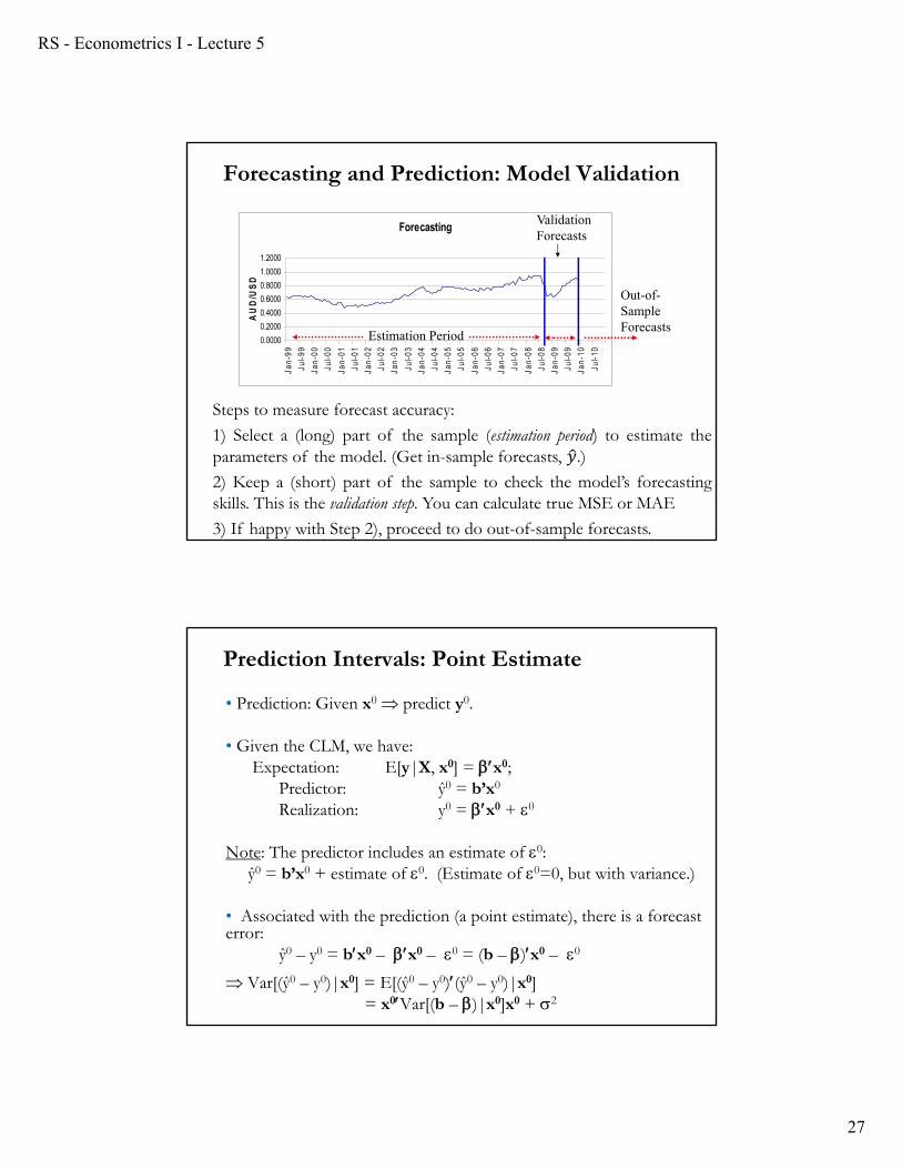
Steps to measure forecast accuracy:

1) Select a (long) part of the sample (estimation period) to estimate theparameters of the model. (Get in-sample forecasts, 𝑦.)

2) Keep a (short) part of the sample to check the model’s forecastingskills. This is the validation step. You can calculate true MSE or MAE

3) If happy with Step 2), proceed to do out-of-sample forecasts.

Forecasting and Prediction: Model Validation

• Prediction: Given x0 predict y0.

• Given the CLM, we have: Expectation: E[y|X, x0] = x0;

Predictor: ŷ0 = b’x0

Realization: y0 = x0 + 0

Note: The predictor includes an estimate of 0: ŷ0 = b’x0 + estimate of 0. (Estimate of 0=0, but with variance.)

• Associated with the prediction (a point estimate), there is a forecast error:

ŷ0 – y0 = bx0 – x0 – 0 = (b – )x0 – 0

Var[(ŷ0 – y0)|x0] = E[(ŷ0 – y0)(ŷ0 – y0)|x0] = x0Var[(b – )|x0]x0 + 2

Prediction Intervals: Point Estimate


28

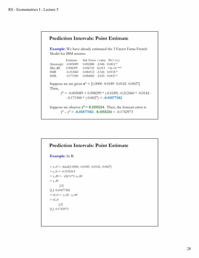
Example: We have already estimated the 3 Factor Fama-French Model for IBM returns:

Estimate Std. Error t value Pr(>|t|) (Intercept) -0.005089 0.002488 -2.046 0.0412 * Mkt_RF 0.908299 0.056722 16.013 <2e-16 ***SMB -0.212460 0.084112 -2.526 0.0118 * HML -0.171500 0.084682 -2.025 0.0433 *

Suppose we are given x0 = [1.0000 -0.0189 -0.0142 -0.0027]Then,

ŷ0 = -0.005089 + 0.908299 * (-0.0189) -0.212460 * -0.0142 -- 0.171500 * (-0.0027) = -0.01877582

Suppose we observe y0 = 0.1555214. Then, the forecast error isŷ0 – y0 = -0.01877582 - 0.1555214 = -0.1742973


Example: In R:

> x_0 <- rbind(1.0000, -0.0189, -0.0142, -0.0027)

> y_0 <- 0.1555214

> y_f0 <- t(b)%*% x_00

> y_f0

[,1]

[1,] -0.01877582

> ef_0 <- y_f0 - y_00

> ef_0

[,1]

[1,] -0.1742973



29

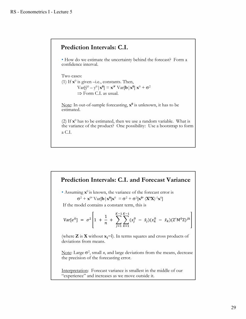
• How do we estimate the uncertainty behind the forecast? Form a confidence interval.

Two cases:(1) If x0 is given –i.e., constants. Then,

Var[ŷ0 – y0|x0] = x0 Var[b|x0] x0 + 2

Form C.I. as usual.

Note: In out-of-sample forecasting, x0 is unknown, it has to be estimated.

(2) If x0 has to be estimated, then we use a random variable. What is the variance of the product? One possibility: Use a bootstrap to form a C.I.

Prediction Intervals: C.I.

• Assuming x0 is known, the variance of the forecast error is 2 + x0’ Var[b|x0]x0 = 2 + 2[x0’ (X’X)-1x0]

If the model contains a constant term, this is

Var 𝑒 𝜎 1 1𝑛 𝑥 �̄� 𝑥 �̄� Z M Z

(where Z is X without x1=ί). In terms squares and cross products of deviations from means.

Note: Large 2, small n, and large deviations from the means, decrease the precision of the forecasting error.

Interpretation: Forecast variance is smallest in the middle of our “experience” and increases as we move outside it.

Prediction Intervals: C.I. and Forecast Variance


30

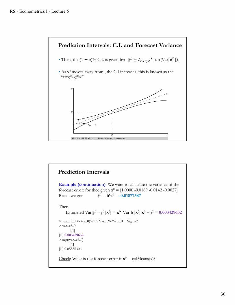
• Then, the (1 α)% C.I. is given by: [ŷ0 tT-k,α/2 * sqrt(Var 𝑒

• As x0 moves away from , the C.I increases, this is known as the “butterfly effect.”

Prediction Intervals: C.I. and Forecast Variance

Example (continuation): We want to calculate the variance of the forecast error: for thee given x0 = [1.0000 -0.0189 -0.0142 -0.0027]Recall we got ŷ0 = b’x0 = -0.01877587

Then,Estimated Var[ŷ0 – y0|x0] = x0 Var[b|x0] x0 + s2 = 0.003429632

> var_ef_0 <- t(x_0)%*% Var_b%*% x_0 + Sigma2> var_ef_0

[,1][1,] 0.003429632> sqrt(var_ef_0)

[,1][1,] 0.05856306

Check: What is the forecast error if x0 = colMeans(x)?

Prediction Intervals


31

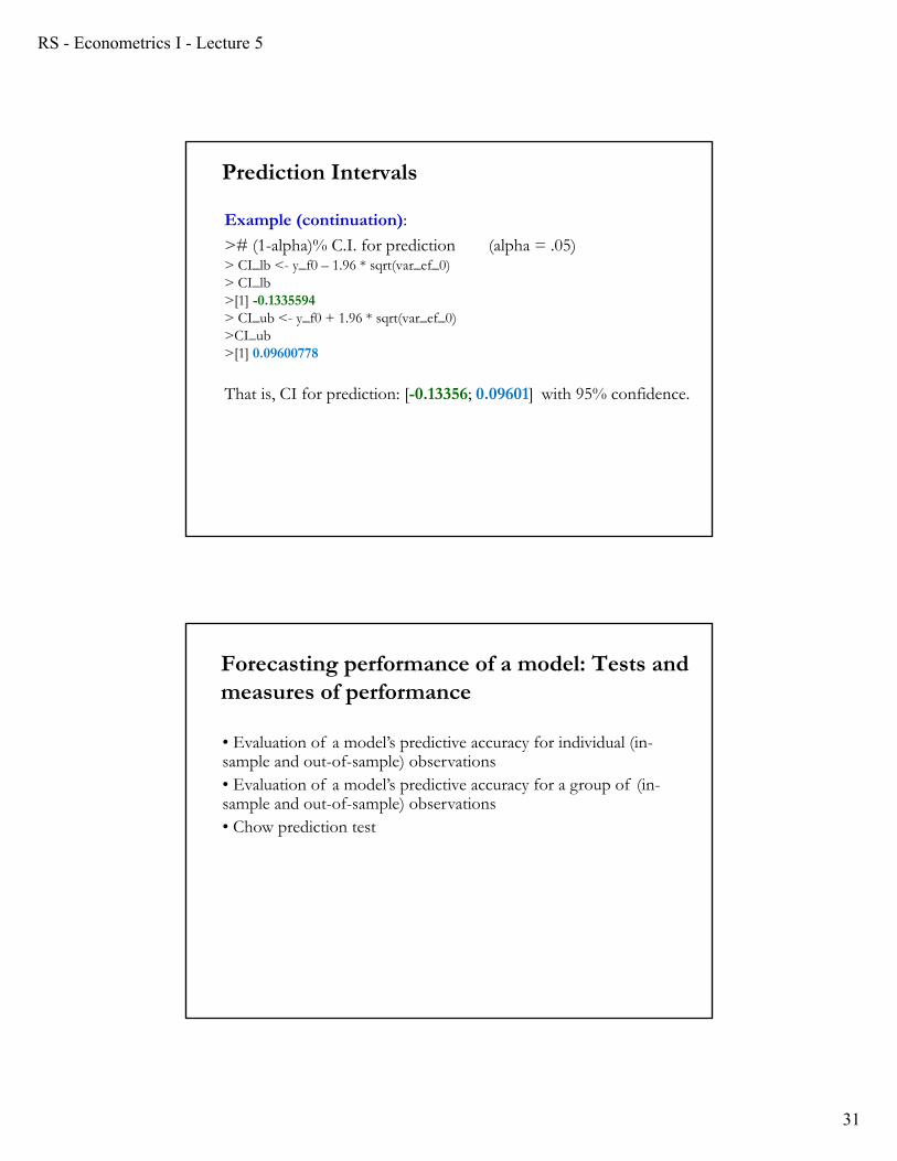
Example (continuation):

># (1-alpha)% C.I. for prediction (alpha = .05)> CI_lb <- y_f0 – 1.96 * sqrt(var_ef_0) > CI_lb>[1] -0.1335594> CI_ub <- y_f0 + 1.96 * sqrt(var_ef_0)>CI_ub>[1] 0.09600778

That is, CI for prediction: [-0.13356; 0.09601] with 95% confidence.

Prediction Intervals

Forecasting performance of a model: Tests and measures of performance

• Evaluation of a model’s predictive accuracy for individual (in-sample and out-of-sample) observations• Evaluation of a model’s predictive accuracy for a group of (in-sample and out-of-sample) observations • Chow prediction test


32

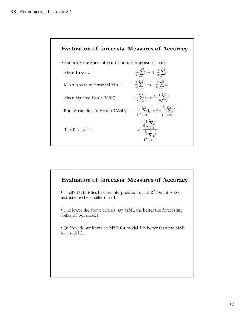
• Summary measures of out-of-sample forecast accuracy

mT

Tii

mT

Tiii e

myy

m11

1)ˆ(

1

mT

Tii

mT

Tiii e

myy

m11

||1

|ˆ|1

mT

Tii

mT

Tiii e

myy

m1

22

1

1)ˆ(

1

Mean Error =

Mean Absolute Error (MAE) =

Root Mean Square Error (RMSE) =

mT

Tii

mT

Tiii e

myy

m1

22

1

1)ˆ(

1Mean Squared Error (MSE) =

T

ii

mT

Tii

yT

em

U

1

2

1

2

1

1

Theil’s U-stat =

Evaluation of forecasts: Measures of Accuracy

• Theil’s U statistics has the interpretation of an R2. But, it is not restricted to be smaller than 1.

• The lower the above criteria, say MSE, the better the forecasting ability of our model.

• Q: How do we know an MSE for model 1 is better than the MSE for model 2?



33

Example: We want to check the forecast accuracy of the 3 FF Factor Model for IBM returns. We estimate the model using only 1973 to 2017 data (T=539), leaving 2018-2020 (30 observations) for validation of predictions.> T0 <- 1

> T1 <- 539

> T2 <- T1+1

> y1 <- y[T0:T1]

> x1 <- x[T0:T1,]

> fit2 <- lm(y1~ x1-1)

> summary(fit2)

Coefficients:


x1 -0.003848 0.002571 -1.497 0.13510

x1Mkt_RF0.865579 0.059386 14.575 < 2e-16 ***

x1SMB -0.224914 0.085505 -2.630 0.00877 **

x1HML -0.230838 0.090251 -2.558 0.01081 *


Example (continuation): We condition on the observed data from 2018: Jan to 2020: Jun.> x_0 <- x[T2:T,]

> y_0 <- y[T2:T]

> y_f0 <- x_0%*% b1

> ef_0 <- y_f0 - y_0

> mes_ef_0 <- sum(ef_0^2)/nrow(x_0)

> mes_ef_0

[1] 0.003703207

> mae_ef_0 <- sum(abs(ef_0))/nrow(x_0)

> mae_ef_0

[1] 0.04518326

That is, MSE = 0.003703207

MAE = 0.04518326



34

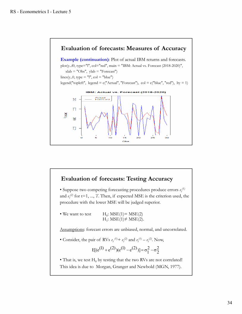
Example (continuation): Plot of actual IBM returns and forecasts.plot(y_f0, type="l", col="red", main = "IBM: Actual vs. Forecast (2018-2020)",

xlab = "Obs", ylab = "Forecast")

lines(y_0, type = "l", col = "blue")

legend("topleft", legend = c("Actual", "Forecast"), col = c("blue", "red"), lty = 1)


• Suppose two competing forecasting procedures produce errors et(1)

and et(2) for t=1, ..., T. Then, if expected MSE is the criterion used, the

procedure with the lower MSE will be judged superior.

• We want to test H0: MSE(1)= MSE(2) H1: MSE(1)≠ MSE(2).

Assumptions: forecast errors are unbiased, normal, and uncorrelated.

• Consider, the pair of RVs et(1)+ et

(2) and et(1) – et

(2). Now,

• That is, we test H0 by testing that the two RVs are not correlated!

This idea is due to Morgan, Granger and Newbold (MGN, 1977).

22

21)])2(e)1(e)()2(e)1(e[(E

Evaluation of forecasts: Testing Accuracy


35

• There is a simpler way to do the MGN test. Let,xt = et

(1) + et(2)

zt = et(1) – et

(2)

(1) Do a regression: xt = β zt + εt

(2) Test H0: β = 0 a simple t-test.

The MGN test statistic is exactly the same as that for testing the null hypothesis that β = 0 in this regression (recall: b = (X′X)-1X′y). This is the approach taken by Harvey, Leybourne and Newbold (1997).

• If the assumptions are violated, these tests have problems.

• A non-parametric HLN variation: Spearman’s rank test for zero correlation between xt and zt.


Example: We produce IBM returns one-step-ahead forecasts for 2018-2020 using the 3 FF Factor Model for IBM returns:

(IBMRet – rf)t = 0 + 1 (MktRet – rf)t + 2 SMBt + 3 HMLt + t

Taking expectations at time t+1, conditioning on time t information set, It ={(MktRet – rf)t, SMBt, HMLt}

E[(IBMRet – rf)t+1|It ] = 0 + 1 E[(MktRet – rf)t+1|It ] ++ 2 E[SMBt+1|It ] + 3 E[HMLt+1|It ]

In order to produce forecast, we will make a naive assumption: The best forecast for the FF factors is the previous observation. Then,

E[(IBMRet – rf)t+1|It ] = 0 + 1 (MktRet – rf)t + 2 SMBt + 3 HMLt.

Now, replacing the by the estimated b, we have our one-step-ahead forecasts.



36

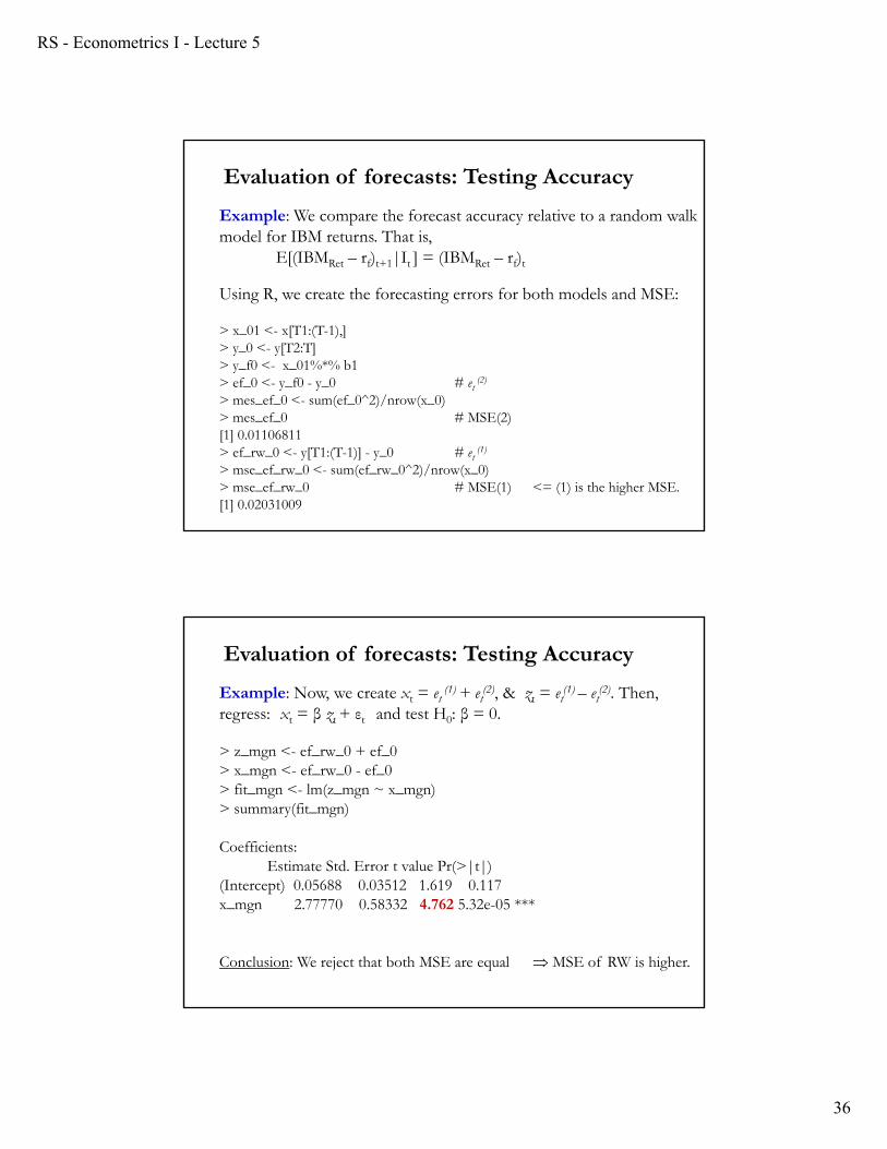
Example: We compare the forecast accuracy relative to a random walk model for IBM returns. That is,

E[(IBMRet – rf)t+1|It ] = (IBMRet – rf)t

Using R, we create the forecasting errors for both models and MSE:

> x_01 <- x[T1:(T-1),]> y_0 <- y[T2:T]> y_f0 <- x_01%*% b1> ef_0 <- y_f0 - y_0 # et

(2)

> mes_ef_0 <- sum(ef_0^2)/nrow(x_0)> mes_ef_0 # MSE(2)[1] 0.01106811> ef_rw_0 <- y[T1:(T-1)] - y_0 # et

(1)

> mse_ef_rw_0 <- sum(ef_rw_0^2)/nrow(x_0)> mse_ef_rw_0 # MSE(1) <= (1) is the higher MSE.[1] 0.02031009


Example: Now, we create xt = et(1) + et

(2), & zt = et(1) – et

(2). Then, regress: xt = β zt + εt and test H0: β = 0.

> z_mgn <- ef_rw_0 + ef_0> x_mgn <- ef_rw_0 - ef_0> fit_mgn <- lm(z_mgn ~ x_mgn)> summary(fit_mgn)


(Intercept) 0.05688 0.03512 1.619 0.117 x_mgn 2.77770 0.58332 4.762 5.32e-05 ***

Conclusion: We reject that both MSE are equal MSE of RW is higher.



37

3

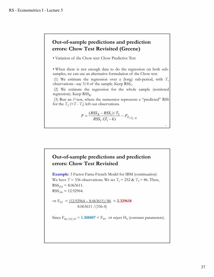
• Variation of the Chow test: Chow Predictive Test

• When there is not enough data to do the regression on both sub-samples, we can use an alternative formulation of the Chow test.(1) We estimate the regression over a (long) sub-period, with T1observations –say 3/4 of the sample. Keep RSS1.(2) We estimate the regression for the whole sample (restrictedregression). Keep RSSR.(3) Run an F-test, where the numerator represents a “predicted” RSSfor the T2 (=T - T1) left out observations.

kTTR F

kTRSS

TRSSRSSF

12 ,

11

21 ~)/(

/)(

Out-of-sample predictions and prediction errors: Chow Test Revisited (Greene)

Out-of-sample predictions and prediction errors: Chow Test Revisited

Example: 3 Factor Fama-French Model for IBM (continuation)We have T = 336 observations. We set T1 = 252 & T2 = 86. Then,RSS252 = 8.063611. RSS336 = 12.92964.

FFF = (12.92964 – 8.063611)/86 = 2.329618 8.063611 /(336-4)

Since F86, 332, 05 = 1.308807 < FFF reject H0 (constant parameters).

Lecture 5 Functional Form and Prediction

Documents

Transcript of Lecture 5 Functional Form and Prediction