LECTURE 3 – SU(2) - Science and Technology Facilities ...hep · LECTURE 3 – SU(2) Contents ......
36
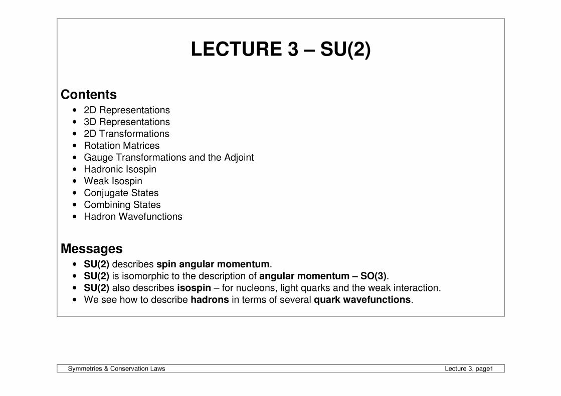
Symmetries & Conservation Laws Lecture 3, page1 LECTURE 3 – SU(2) Contents • 2D Representations • 3D Representations • 2D Transformations • Rotation Matrices • Gauge Transformations and the Adjoint • Hadronic Isospin • Weak Isospin • Conjugate States • Combining States • Hadron Wavefunctions Messages • SU(2) describes spin angular momentum. • SU(2) is isomorphic to the description of angular momentum – SO(3). • SU(2) also describes isospin – for nucleons, light quarks and the weak interaction. • We see how to describe hadrons in terms of several quark wavefunctions.
Transcript of LECTURE 3 – SU(2) - Science and Technology Facilities ...hep · LECTURE 3 – SU(2) Contents ......
Symmetries & Conservation Laws Lecture 3, page1
LECTURE 3 – SU(2)
Contents • 2D Representations
• 3D Representations
• 2D Transformations
• Rotation Matrices
• Gauge Transformations and the Adjoint
• Hadronic Isospin
• Weak Isospin
• Conjugate States
• Combining States
• Hadron Wavefunctions
Messages • SU(2) describes spin angular momentum.
• SU(2) is isomorphic to the description of angular momentum – SO(3).
• SU(2) also describes isospin – for nucleons, light quarks and the weak interaction.
• We see how to describe hadrons in terms of several quark wavefunctions.
Symmetries & Conservation Laws Lecture 3, page2
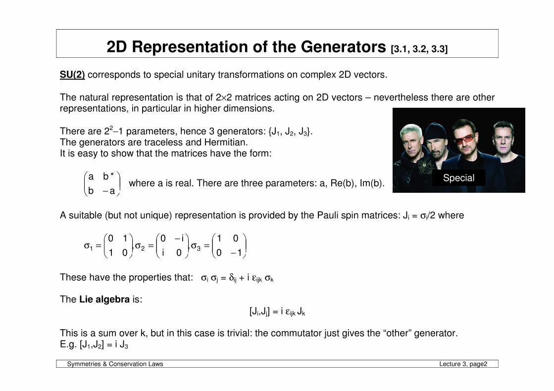
2D Representation of the Generators [3.1, 3.2, 3.3] SU(2) corresponds to special unitary transformations on complex 2D vectors.
The natural representation is that of 2×2 matrices acting on 2D vectors – nevertheless there are other representations, in particular in higher dimensions.
There are 22−1 parameters, hence 3 generators: {J1, J2, J3}. The generators are traceless and Hermitian. It is easy to show that the matrices have the form:
− ab
*ba where a is real. There are three parameters: a, Re(b), Im(b).
A suitable (but not unique) representation is provided by the Pauli spin matrices: Ji = σi/2 where
−=σ
−=σ
=σ
10
01,
0i
i0,
01
10321
These have the properties that: σi σj = δij + i εijk σk The Lie algebra is:
[Ji,Jj] = i εijk Jk
This is a sum over k, but in this case is trivial: the commutator just gives the “other” generator. E.g. [J1,J2] = i J3
Special

Symmetries & Conservation Laws Lecture 3, page3
Quantum Numbers [3.2, 3.3] A Casimir Operator is one which commutes with all other generators. In SU(2) there is just one Casimir: J2 = J1
2 + J22 + J3
2 Since [J2,J3] = 0, they can have simultaneous observables and can provide suitable QM eigenvalues by which to label states.
We can define Raising & Lowering Operators: J± = J1 ± iJ2
Can show [J3,J±] = ±J±
Define eigenstates |j m> with their corresponding eigenvalues:
J2 |j m> = j(j+1) |j m>
J3 |j m> = m |j m>
Recall from angular momentum in QM, J± generates different states within a multiplet:
J3 J±|j m> = (m±1) J±|j m> and
J± |j m> = )1mj)(mj( +±m |j m±1>
Exercise
Prove [J2,Ji] = 0 and [J3,J±] = ±J±
And J3 J±|j m> = (m±1) J±|j m> and J± |j m> = )1mj)(mj( +±m |j m±1>
And J± |j ±j> = 0
Symmetries & Conservation Laws Lecture 3, page4
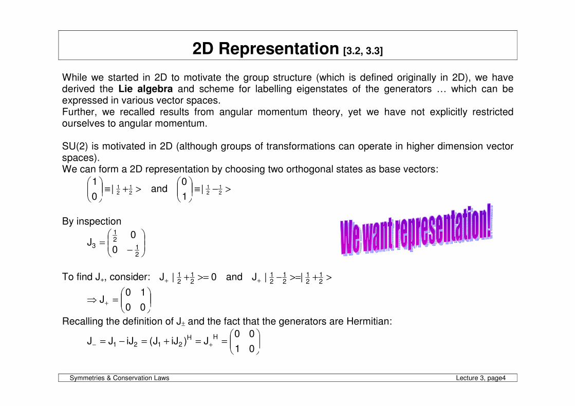
2D Representation [3.2, 3.3] While we started in 2D to motivate the group structure (which is defined originally in 2D), we have derived the Lie algebra and scheme for labelling eigenstates of the generators … which can be expressed in various vector spaces. Further, we recalled results from angular momentum theory, yet we have not explicitly restricted ourselves to angular momentum. SU(2) is motivated in 2D (although groups of transformations can operate in higher dimension vector spaces). We can form a 2D representation by choosing two orthogonal states as base vectors:
>+≡
21
21|
0
1 and >−≡
21
21|
1
0
By inspection
−=
21
21
30
0J
To find J+, consider: 0|J21
21 >=++ and >+>=−+ 2
121
21
21 ||J
=⇒ +
00
10J
Recalling the definition of J± and the fact that the generators are Hermitian:
==+=−= +−
01
00J)iJJ(iJJJ
HH2121
Symmetries & Conservation Laws Lecture 3, page5
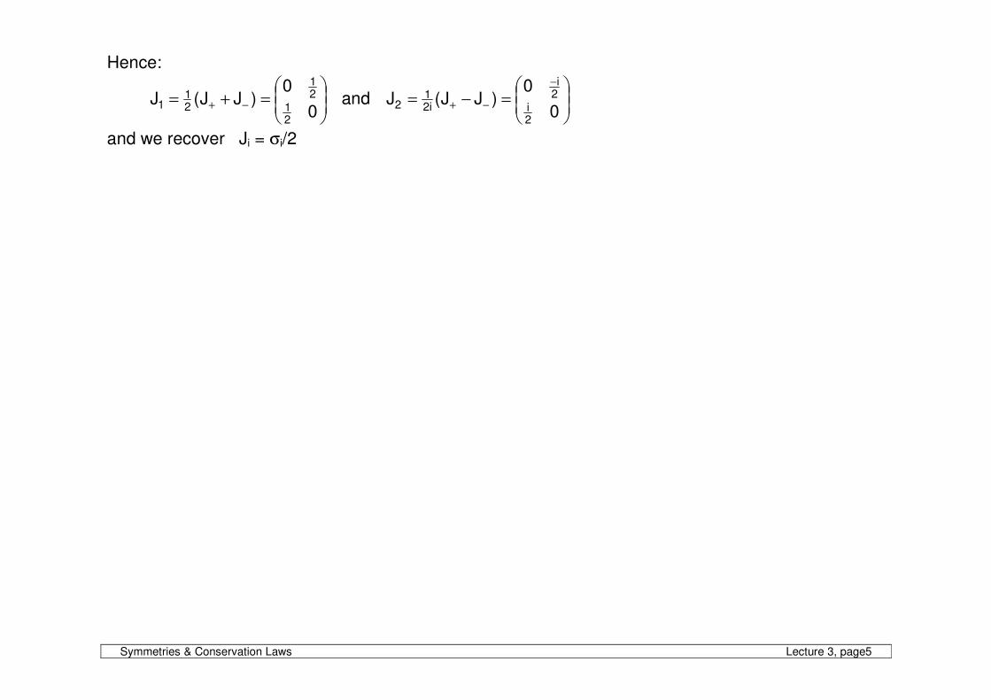
Hence:
=+= −+
0
0)JJ(J
21
21
21
1 and
=−=
−
−+0
0)JJ(J
2i
2i
i21
2
and we recover Ji = σi/2
Symmetries & Conservation Laws Lecture 3, page6
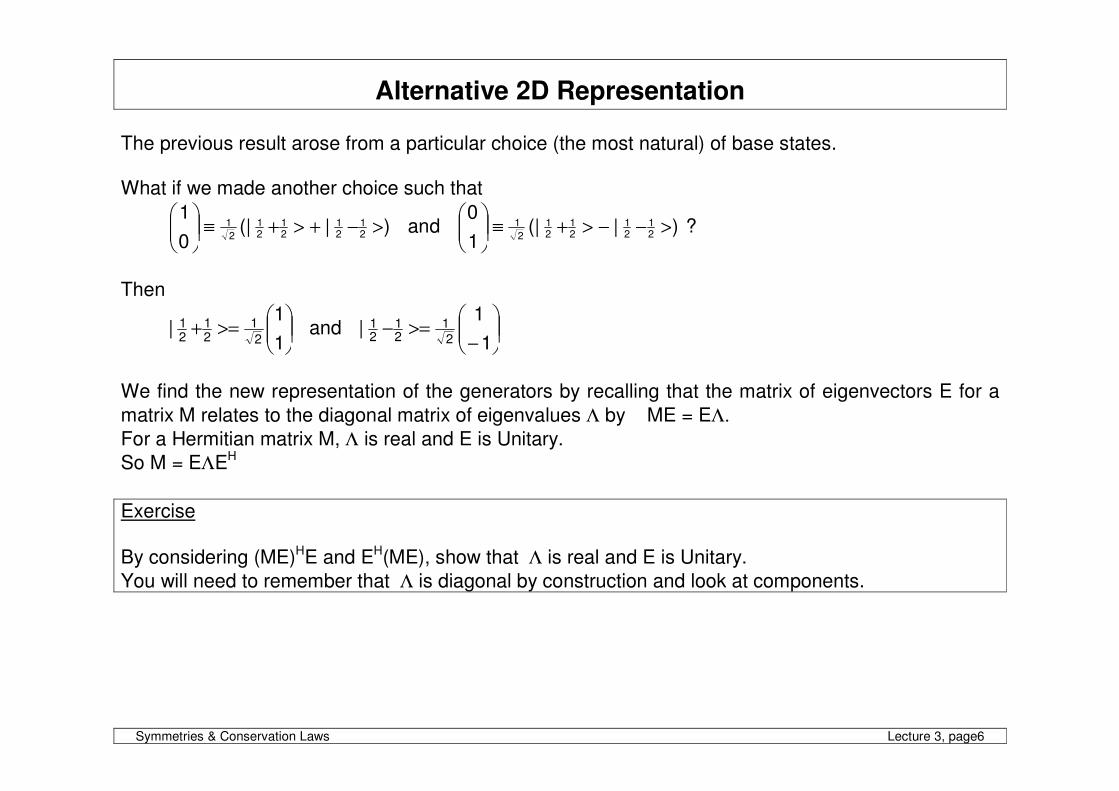
Alternative 2D Representation The previous result arose from a particular choice (the most natural) of base states. What if we made another choice such that
)|(|0
121
21
21
21
2
1 >−+>+≡
and )|(|
1
021
21
21
21
2
1 >−−>+≡
?
Then
>=+
1
1|
2
121
21 and
−>=−
1
1|
2
121
21
We find the new representation of the generators by recalling that the matrix of eigenvectors E for a
matrix M relates to the diagonal matrix of eigenvalues Λ by ME = EΛ.
For a Hermitian matrix M, Λ is real and E is Unitary.
So M = EΛEH
Exercise
By considering (ME)HE and EH(ME), show that Λ is real and E is Unitary.
You will need to remember that Λ is diagonal by construction and look at components.
Symmetries & Conservation Laws Lecture 3, page7
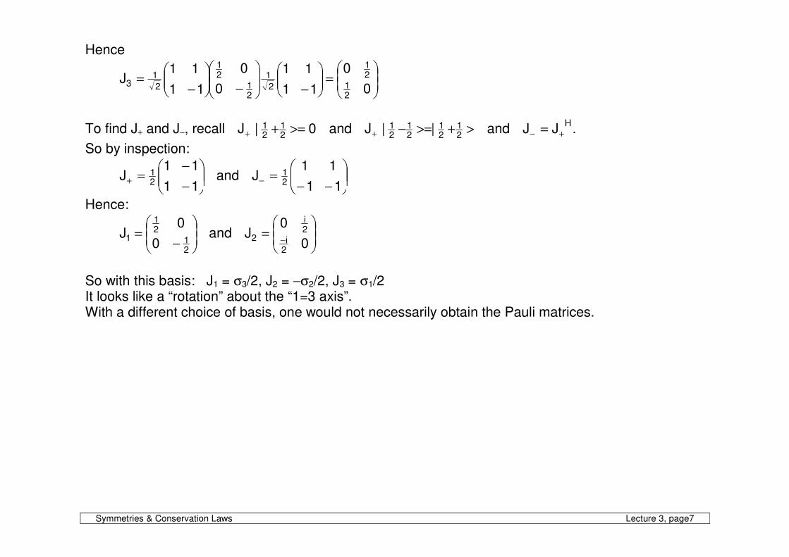
Hence
=
−
−
−=
0
0
11
11
0
0
11
11J
21
21
2
1
21
21
2
13
To find J+ and J−, recall 0|J21
21 >=++ and >+>=−+ 2
121
21
21 ||J and
HJJ +− = .
So by inspection:
−
−=+
11
11J
21 and
−−=−
11
11J
21
Hence:
−=
21
21
10
0J and
=
− 0
0J
2i
2i
2
So with this basis: J1 = σ3/2, J2 = −σ2/2, J3 = σ1/2 It looks like a “rotation” about the “1=3 axis”. With a different choice of basis, one would not necessarily obtain the Pauli matrices.
Symmetries & Conservation Laws Lecture 3, page8
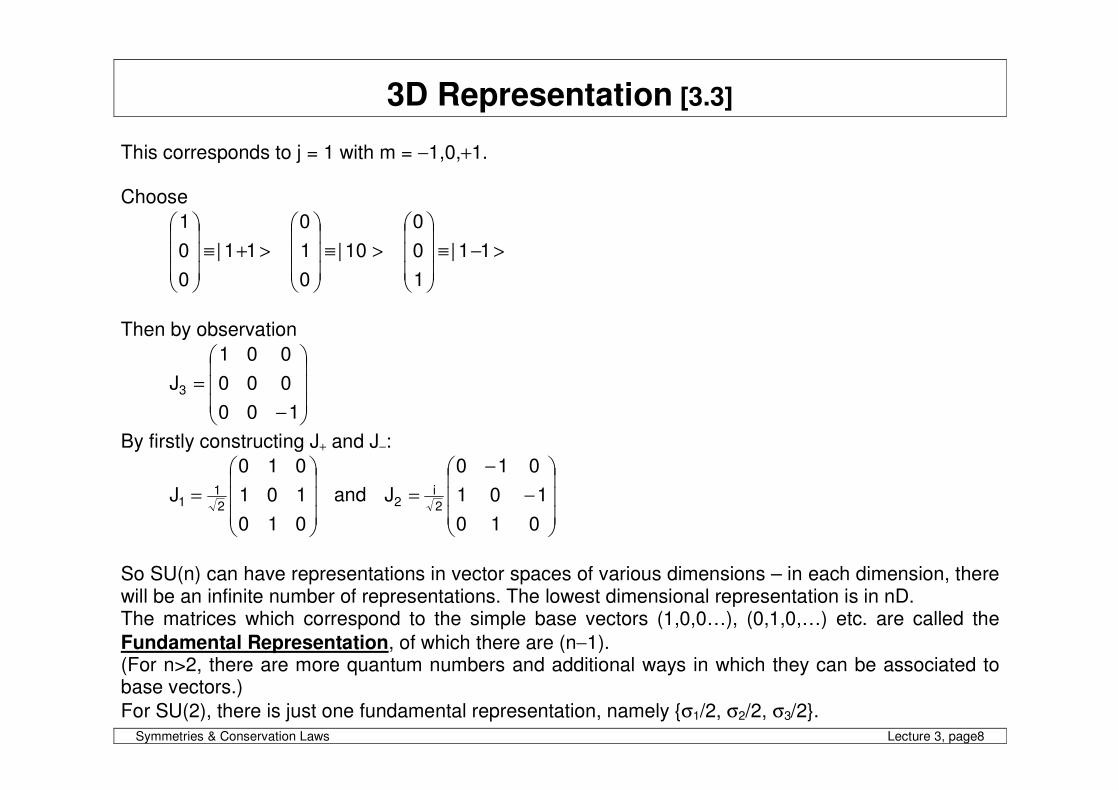
3D Representation [3.3]
This corresponds to j = 1 with m = −1,0,+1. Choose
>+≡
11|
0
0
1
>≡
10|
0
1
0
>−≡
11|
1
0
0
Then by observation
−
=
100
000
001
J3
By firstly constructing J+ and J−:
=
010
101
010
J2
11 and
−
−
=
010
101
010
J2
i2
So SU(n) can have representations in vector spaces of various dimensions – in each dimension, there will be an infinite number of representations. The lowest dimensional representation is in nD. The matrices which correspond to the simple base vectors (1,0,0…), (0,1,0,…) etc. are called the
Fundamental Representation, of which there are (n−1). (For n>2, there are more quantum numbers and additional ways in which they can be associated to base vectors.)
For SU(2), there is just one fundamental representation, namely {σ1/2, σ2/2, σ3/2}.
Symmetries & Conservation Laws Lecture 3, page9
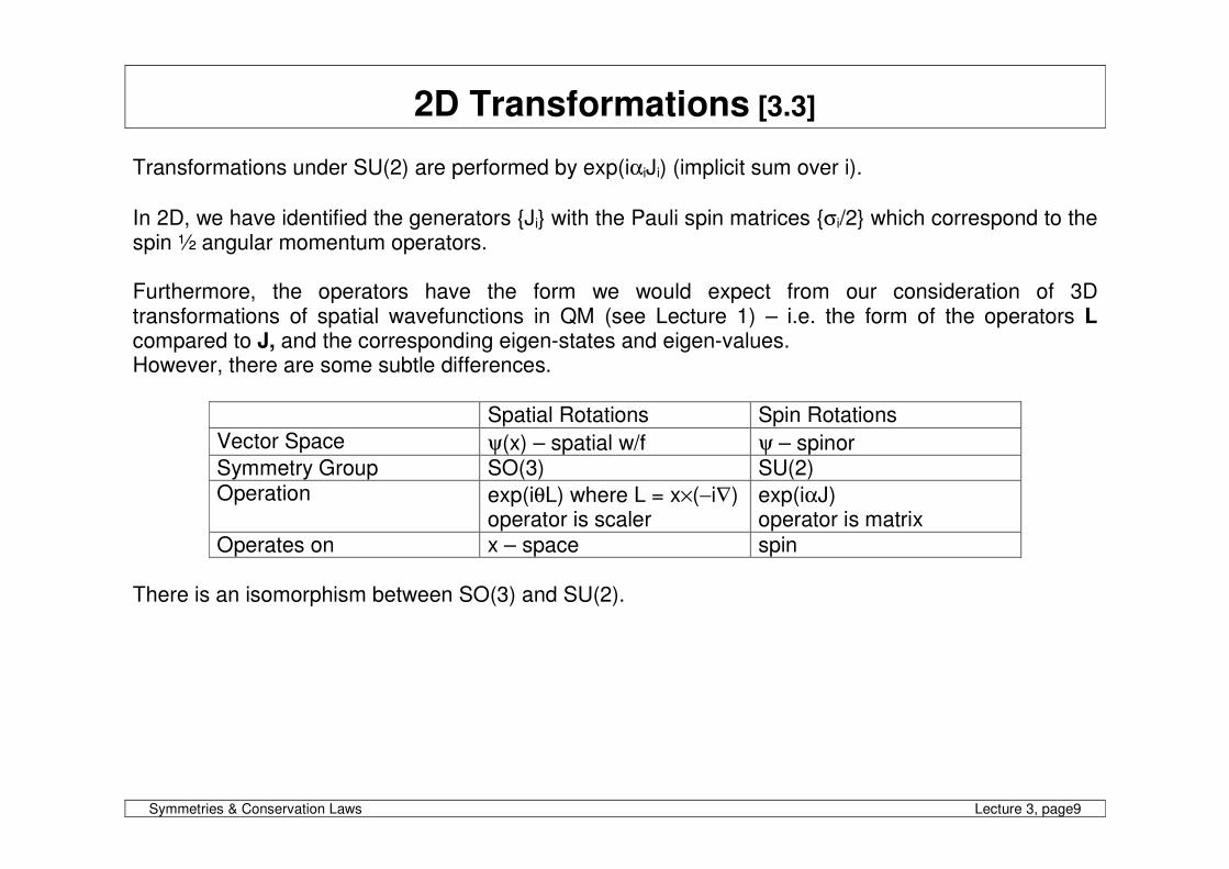
2D Transformations [3.3]
Transformations under SU(2) are performed by exp(iαiJi) (implicit sum over i).
In 2D, we have identified the generators {Ji} with the Pauli spin matrices {σi/2} which correspond to the spin ½ angular momentum operators. Furthermore, the operators have the form we would expect from our consideration of 3D transformations of spatial wavefunctions in QM (see Lecture 1) – i.e. the form of the operators L compared to J, and the corresponding eigen-states and eigen-values. However, there are some subtle differences.
Spatial Rotations Spin Rotations
Vector Space ψ(x) – spatial w/f ψ – spinor Symmetry Group SO(3) SU(2) Operation exp(iθL) where L = x×(−i∇)
operator is scaler exp(iαJ) operator is matrix
Operates on x – space spin There is an isomorphism between SO(3) and SU(2).
Symmetries & Conservation Laws Lecture 3, page10
The transformation operator is U = exp(iαiσi/2).
Writing αi = 2ωni, where n is a unit vector, gives U = exp(iωn⋅σ). Expanding the exponential:
U = 1 + (iωn⋅σ) + (iωn⋅σ)2/2! + (iωn⋅σ)3/3! …
(n⋅σ)2 = n12 σ1
2+ … + n1 n2 (σ1 σ2 +σ2 σ1)+ ...
σ12= 1 and (σ1 σ2 +σ2 σ1) = 0 ⇒ (n⋅σ)2 = n1
2 + n22 + n3
2 = 1 So
U = {1 − ω2/2! + ω4/4! + …} + i{ω − ω3/3! + ω5/5! – …} n⋅σ = cos ω + i sin ω n⋅σ
σ⋅+=σ⋅ θθθ nsinicos)niexp(222
We can now prove the Lie nature of SU(2) explicitly. We should expect that the product of two operators is a third one of a similar form, where the parameters of the result are a function of the parameters of the first two operations.
)bsini)(cosasini(cos)biexp()aiexp( σ⋅β+βσ⋅α+α=σ⋅βσ⋅α
Using σ⋅×+⋅=σ⋅σ⋅ biababa , which is derived from σi σj = δij + i εijk σk
σ⋅+≡σ⋅αβ+βα+×+⋅βα−βα=
σ⋅αβ+σ⋅βα+σ⋅×+⋅βα−βα=σ⋅βσ⋅α
iSC}bcossinacossinba{i}basinsincos{cos
)bcossinacos(sini)biaba(sinsincoscos)biexp()aiexp(
To show that this has the form σ⋅γ+γ csinicos , it is sufficient to show that C2+S2 = 1 – this
straightforward, albeit tedious !
Symmetries & Conservation Laws Lecture 3, page11
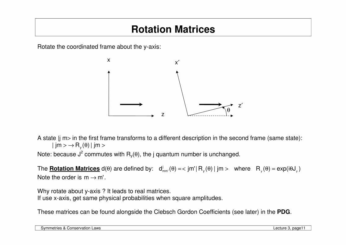
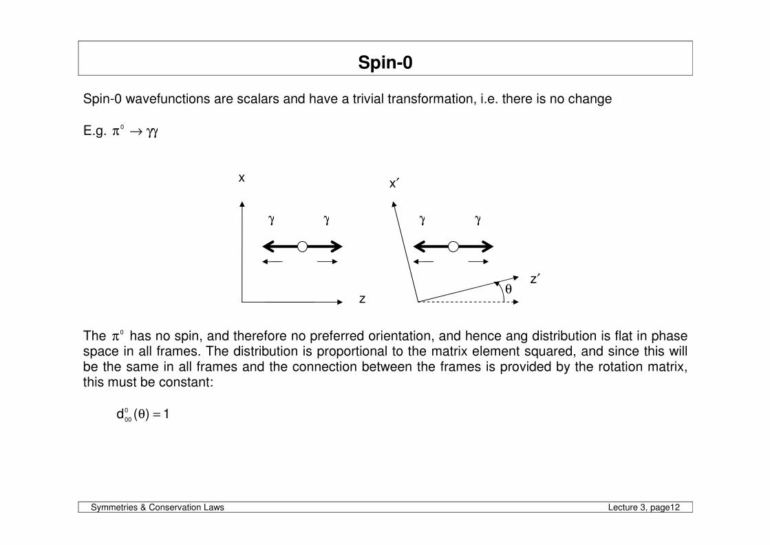
Rotation Matrices Rotate the coordinated frame about the y-axis:
A state |j m> in the first frame transforms to a different description in the second frame (same state): >θ→> jm|)(Rjm| y
Note: because J2 commutes with Ry(θ), the j quantum number is unchanged.
The Rotation Matrices d(θ) are defined by: >θ<=θ jm|)(R|'jm)(d y
j
'mm where )Jiexp()(Ryy
θ=θ
Note the order is 'mm → . Why rotate about y-axis ? It leads to real matrices. If use x-axis, get same physical probabilities when square amplitudes. These matrices can be found alongside the Clebsch Gordon Coefficients (see later) in the PDG.
θ z
x x′
z′
Symmetries & Conservation Laws Lecture 3, page12
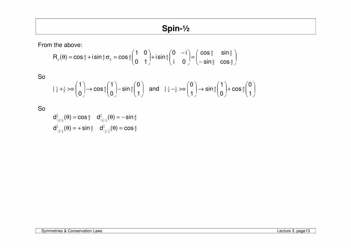
Spin-0 Spin-0 wavefunctions are scalars and have a trivial transformation, i.e. there is no change
E.g. γγ→π0
The 0π has no spin, and therefore no preferred orientation, and hence ang distribution is flat in phase space in all frames. The distribution is proportional to the matrix element squared, and since this will be the same in all frames and the connection between the frames is provided by the rotation matrix, this must be constant:
1)(d0
00=θ
θ z
x x′
z′
γ γ γ γ
Symmetries & Conservation Laws Lecture 3, page13
Spin-½ From the above:
−=
−+
=σ+=θ
θθ
θθ
θθθθ
22
22
22222ycossin
sincos
0i
i0sini
10
01cossinicos)(R
So
−
→
>≡+ θθ
1
0sin
0
1cos
0
1| 222
1
2
1 and
+
→
>≡− θθ
1
0cos
0
1sin
1
0| 222
1
2
1
So
2cos)(d21
21
21
θ
++=θ 2sin)(d2
1
21
21
θ
−+−=θ
2sin)(d21
21
21
θ
+−+=θ 2cos)(d2
1
21
21
θ
−−=θ
Symmetries & Conservation Laws Lecture 3, page14
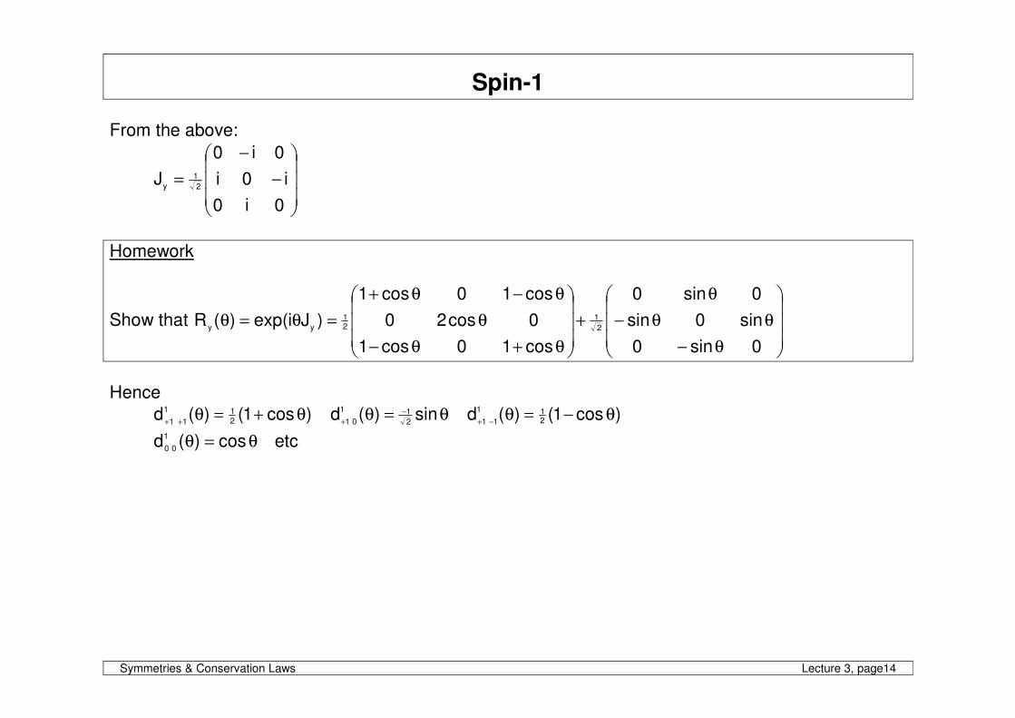
Spin-1 From the above:
−
−
=
0i0
i0i
0i0
J2
1
y
Homework
Show that
θ−
θθ−
θ
+
θ+θ−
θ
θ−θ+
=θ=θ
0sin0
sin0sin
0sin0
cos10cos1
0cos20
cos10cos1
)Jiexp()(R2
121
yy
Hence
)cos1()(d 2
11
11θ+=θ
++ θ=θ −
+sin)(d
2
11
01 )cos1()(d 2
11
11θ−=θ
−+
θ=θ cos)(d1
00 etc
Symmetries & Conservation Laws Lecture 3, page15
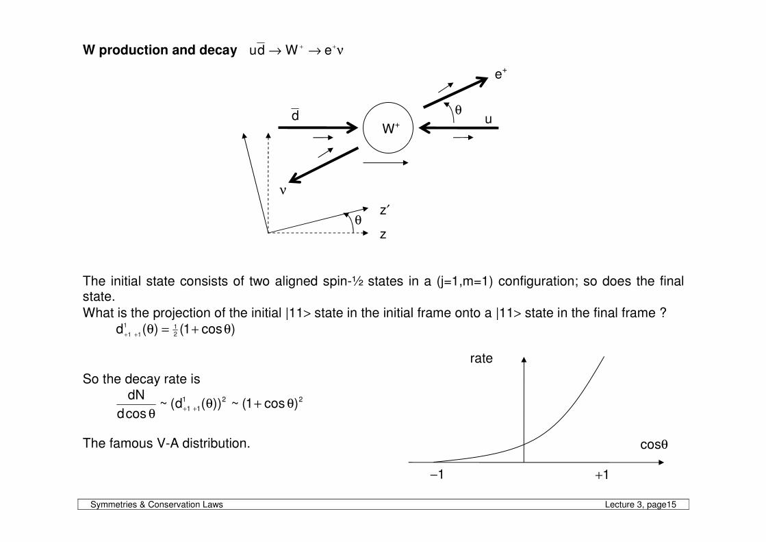
W production and decay ν→→ ++ eWdu
The initial state consists of two aligned spin-½ states in a (j=1,m=1) configuration; so does the final state.
What is the projection of the initial |11> state in the initial frame onto a |11> state in the final frame ?
)cos1()(d 2
11
11θ+=θ
++
So the decay rate is
221
11 )cos1(~))(d(~cosd
dNθ+θ
θ++
The famous V-A distribution.
θ z
z′
ν
W+
θ u d
e+
cosθ
rate
+1 −1
Symmetries & Conservation Laws Lecture 3, page16
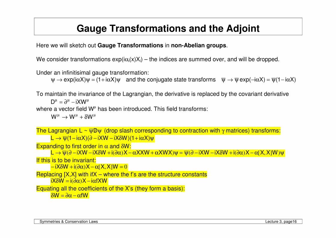
Gauge Transformations and the Adjoint Here we will sketch out Gauge Transformations in non-Abelian groups.
We consider transformations exp(iαi(x)Xi) – the indices are summed over, and will be dropped. Under an infinitisimal gauge transformation:
ψα+=ψα→ψ )Xi1()Xiexp( and the conjugate state transforms )Xi1()Xiexp( α−ψ=α−ψ→ψ
To maintain the invariance of the Lagrangian, the derivative is replaced by the covariant derivative
µµµ −∂= iXWD
where a vector field Wµ has been introduced. This field transforms: µµµ δ+→ WWW
The Lagrangian ψ/ψD~L (drop slash corresponding to contraction with γ matrices) transforms:
ψα+δ−−∂α−ψ→ )Xi1)(WiXiXW)(Xi1(L
Expanding to first order in α and δW: ψα−α∂+δ−−∂ψ=ψα+α−α∂+δ−−∂ψ→ )],[)(())(( WXXXiWiXiXWXWXXXWXiWiXiXWL
If this is to be invariant: 0],[)( =α−α∂+δ− WXXXiWiX
Replacing [X,X] with ifX – where the f’s are the structure constants fXWiXiWiX α−α∂=δ )(
Equating all the coefficients of the X’s (they form a basis): fWW α−α∂=δ
Symmetries & Conservation Laws Lecture 3, page17
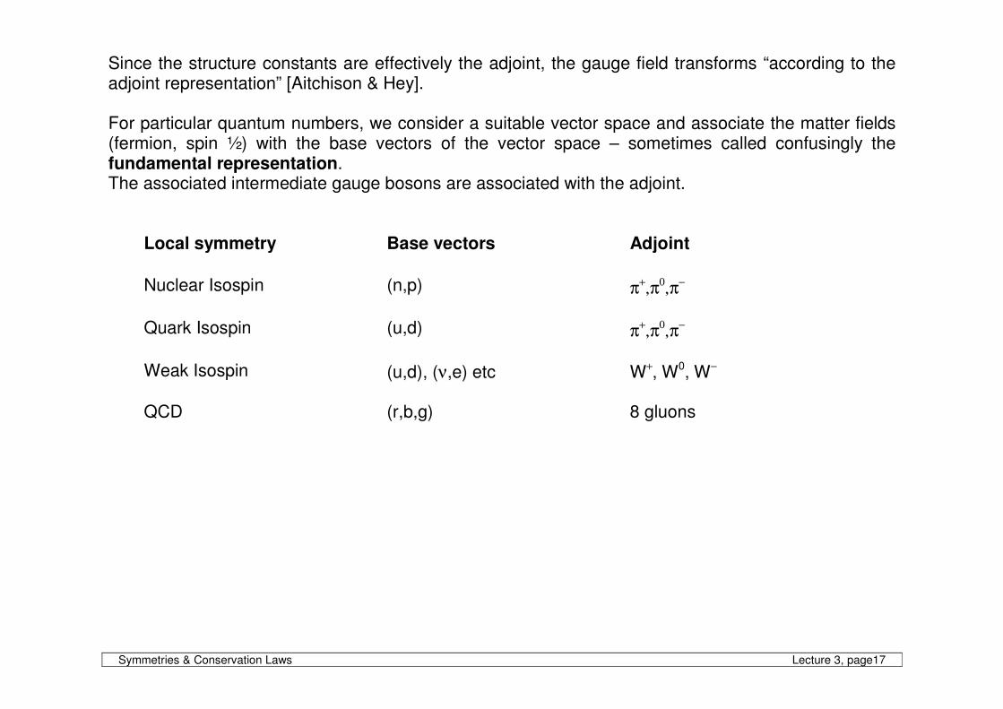
Since the structure constants are effectively the adjoint, the gauge field transforms “according to the adjoint representation” [Aitchison & Hey]. For particular quantum numbers, we consider a suitable vector space and associate the matter fields (fermion, spin ½) with the base vectors of the vector space – sometimes called confusingly the fundamental representation. The associated intermediate gauge bosons are associated with the adjoint.
Local symmetry Base vectors Adjoint
Nuclear Isospin
(n,p)
π+,π0,π− Quark Isospin
(u,d)
π+,π0,π− Weak Isospin
(u,d), (ν,e) etc
W+, W0, W− QCD
(r,b,g)
8 gluons
Symmetries & Conservation Laws Lecture 3, page18
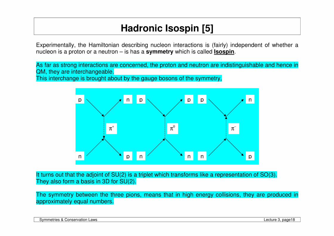
Hadronic Isospin [5] Experimentally, the Hamiltonian describing nucleon interactions is (fairly) independent of whether a nucleon is a proton or a neutron – is has a symmetry which is called Isospin. As far as strong interactions are concerned, the proton and neutron are indistinguishable and hence in QM, they are interchangeable. This interchange is brought about by the gauge bosons of the symmetry,
It turns out that the adjoint of SU(2) is a triplet which transforms like a representation of SO(3). They also form a basis in 3D for SU(2). The symmetry between the three pions, means that in high energy collisions, they are produced in approximately equal numbers.
p
n p
n
π−
p
n n
p
π0
p
n p
n
π+
Symmetries & Conservation Laws Lecture 3, page19
We can treat the nucleon as particle which has two possible states: p or n, and we denote the state by a vector (p,n). In terms of quantum numbers (I,I3) – along the same lines as the angular momentum labels:
Doublet p = (½,+½) n = (½,−½)
Triplet π+ = (1,+1) π0 = (1,0) π− = (1,−1)
In reality, the hadrons are distinguishable (else we would not have been able to label them) – they are distinguished by their electric charge and mass. These break the symmetry of the Hamiltonian, but since the EM effects are ~1/100th the size of the strong interaction, the symmetry is fairly good. By observation, we can write the charge operator:
Q = ½ B + I3
This corresponds to a symmetry U(1)B ⊗ SU(2)I Any complete Hamiltonian contains a Q. Since Q commutes with I3 and I2, so I3 and I2 will correspond to conserved quantum numbers; however Q does not commute with I (vector), and so will not be invariant under general isospin transformations, such as those corresponding to p-n interchange. Historically, a lot was made of this symmetry to understand nucleon scattering and production. We will examine how one can use the “machinery” when we look at the quark model. As an example [5.6], the deuteron is made from a proton and a neutron in a ground-state s-wave (symmetric spatial wave-function). It appears as a single state (no other comparable particles) and this is in an I=0 antisymmetric state. To ensure the complete wave-function for two “identical” particles is antisymmetric, the spins must be in a symmetric state, namely S = 1.
Symmetries & Conservation Laws Lecture 3, page20
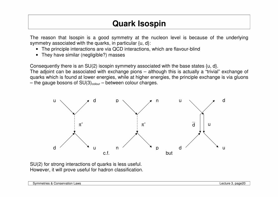
Quark Isospin The reason that Isospin is a good symmetry at the nucleon level is because of the underlying symmetry associated with the quarks, in particular {u, d}:
• The principle interactions are via QCD interactions, which are flavour-blind
• They have similar (negligible?) masses Consequently there is an SU(2) isospin symmetry associated with the base states {u, d}. The adjoint can be associated with exchange pions – although this is actually a “trivial” exchange of quarks which is found at lower energies, while at higher energies, the principle exchange is via gluons – the gauge bosons of SU(3)colour – between colour charges.
c.f. but SU(2) for strong interactions of quarks is less useful. However, it will prove useful for hadron classification.
u
d u
d
u dd
p
n p
n
π+
u
d u
d
π+
Symmetries & Conservation Laws Lecture 3, page21
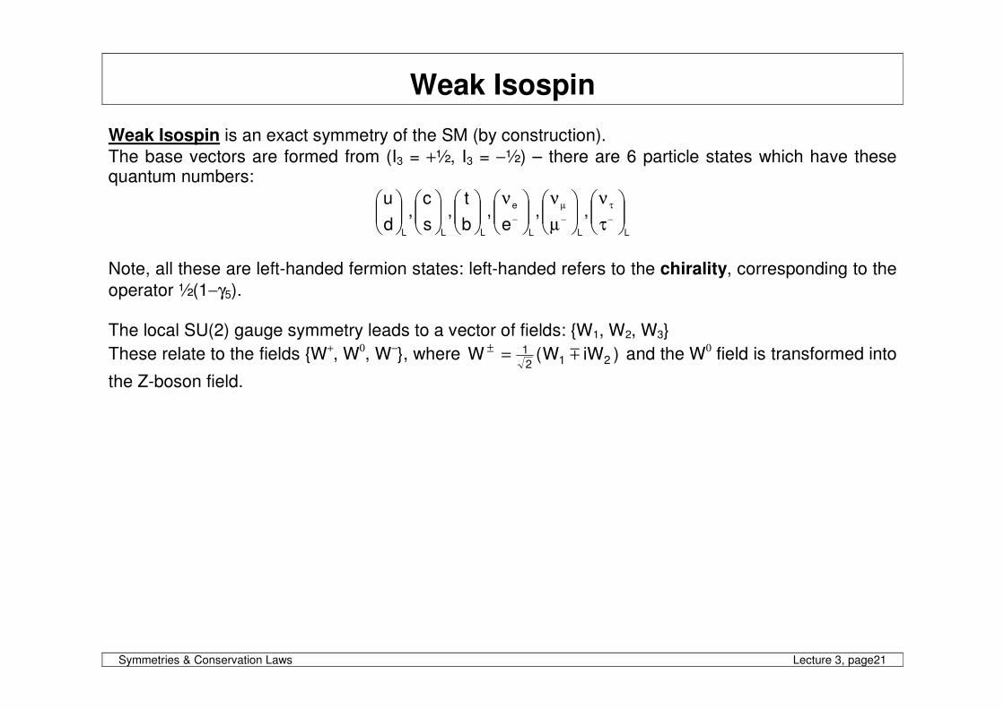
Weak Isospin Weak Isospin is an exact symmetry of the SM (by construction).
The base vectors are formed from (I3 = +½, I3 = −½) – there are 6 particle states which have these quantum numbers:
LLL
e
LLL
,,e
,b
t,
s
c,
d
u
τ
ν
µ
ν
ν
−
τ
−
µ
−
Note, all these are left-handed fermion states: left-handed refers to the chirality, corresponding to the
operator ½(1−γ5). The local SU(2) gauge symmetry leads to a vector of fields: {W1, W2, W3}
These relate to the fields {W+, W0, W−}, where )iWW(W 212
1m=± and the W0 field is transformed into
the Z-boson field.
Symmetries & Conservation Laws Lecture 3, page22
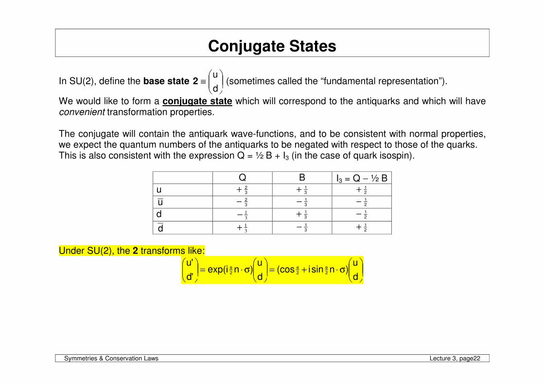
Conjugate States
In SU(2), define the base state
≡
d
u2 (sometimes called the “fundamental representation”).
We would like to form a conjugate state which will correspond to the antiquarks and which will have convenient transformation properties. The conjugate will contain the antiquark wave-functions, and to be consistent with normal properties, we expect the quantum numbers of the antiquarks to be negated with respect to those of the quarks. This is also consistent with the expression Q = ½ B + I3 (in the case of quark isospin).
Q B I3 = Q − ½ B u 3
2+ 31+ 2
1+
u 32− 3
1− 21−
d 3
1− 31+ 2
1−
d 3
1+ 31− 2
1+
Under SU(2), the 2 transforms like:
σ⋅+=
σ⋅=
θθθ
d
u)nsini(cos
d
u)niexp(
'd
'u222
Symmetries & Conservation Laws Lecture 3, page23
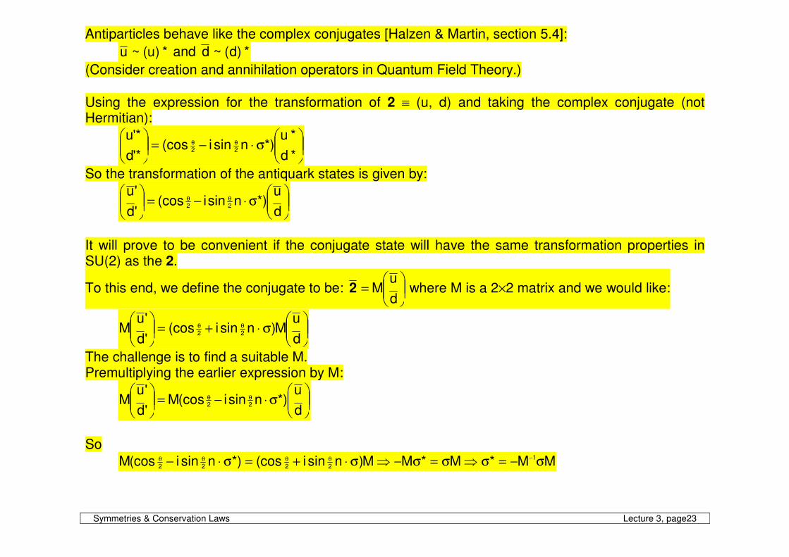
Antiparticles behave like the complex conjugates [Halzen & Martin, section 5.4]:
*)u(~u and *)d(~d
(Consider creation and annihilation operators in Quantum Field Theory.)
Using the expression for the transformation of 2 ≡ (u, d) and taking the complex conjugate (not Hermitian):
σ⋅−=
θθ
*d
*u*)nsini(cos
'*d
'*u22
So the transformation of the antiquark states is given by:
σ⋅−=
θθ
d
u*)nsini(cos
'd
'u22
It will prove to be convenient if the conjugate state will have the same transformation properties in SU(2) as the 2.
To this end, we define the conjugate to be:
=
d
uM2 where M is a 2×2 matrix and we would like:
σ⋅+=
θθ
d
uM)nsini(cos
'd
'uM 22
The challenge is to find a suitable M. Premultiplying the earlier expression by M:
σ⋅−=
θθ
d
u*)nsini(cosM
'd
'uM 22
So
MM*M*MM)nsini(cos*)nsini(cosM 1
2222 σ−=σ⇒σ=σ−⇒σ⋅+=σ⋅− −θθθθ
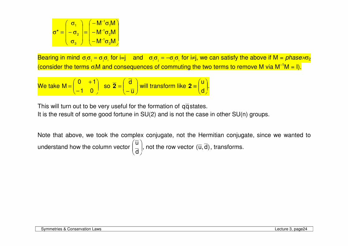
Symmetries & Conservation Laws Lecture 3, page24
σ−
σ−
σ−
=
σ
σ−
σ
=σ−
−
−
MM
MM
MM
*
3
1
2
1
1
1
3
2
1
Bearing in mind ijji
σσ=σσ for i=j and ijji
σσ−=σσ for i≠j, we can satisfy the above if M = phase×σ2
(consider the terms σiM and consequences of commuting the two terms to remove M via M−1M = I).
We take
−
+=
01
10M so
−=
u
d2 will transform like
≡
d
u2 .
This will turn out to be very useful for the formation of qq states.
It is the result of some good fortune in SU(2) and is not the case in other SU(n) groups. Note that above, we took the complex conjugate, not the Hermitian conjugate, since we wanted to
understand how the column vector
d
u, not the row vector )d,u( , transforms.
Symmetries & Conservation Laws Lecture 3, page25
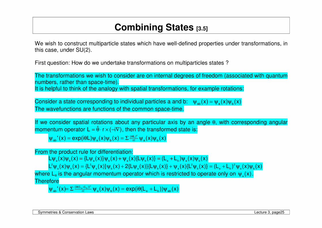
Combining States [3.5] We wish to construct multiparticle states which have well-defined properties under transformations, in this case, under SU(2). First question: How do we undertake transformations on multiparticles states ? The transformations we wish to consider are on internal degrees of freedom (associated with quantum numbers, rather than space-time). It is helpful to think of the analogy with spatial transformations, for example rotations: Consider a state corresponding to individual particles a and b: )x()x()x( baab ψψ=ψ
The wavefunctions are functions of the common space-time.
If we consider spatial rotations about any particular axis by an angle θ, with corresponding angular
momentum operator )i(rˆL ∇−×⋅θ= , then the transformed state is:
)x()x()x()x()Liexp()x(' ba!n
)Li(
baab
n
ψψΣ=ψψθ=ψ θ
From the product rule for differentiation:
)x()x()LL()}x(L){x()x()}x(L{)x()x(Lbababababa
ψψ+=ψψ+ψψ=ψψ
)x()x()LL()}x(L){x()}x(L)}{x(L{2)x()}x(L{)x()x(Lba
2
bab
2
ababa
2
ba
2 ψψ+=ψψ+ψψ+ψψ=ψψ
where La is the angular momentum operator which is restricted to operate only on )x(a
ψ .
Therefore
)x())LL(iexp()x()x()x(' abbaba!n
))LL(i(
ab
nba ψ+θ=ψψΣ=ψ +θ
Symmetries & Conservation Laws Lecture 3, page26
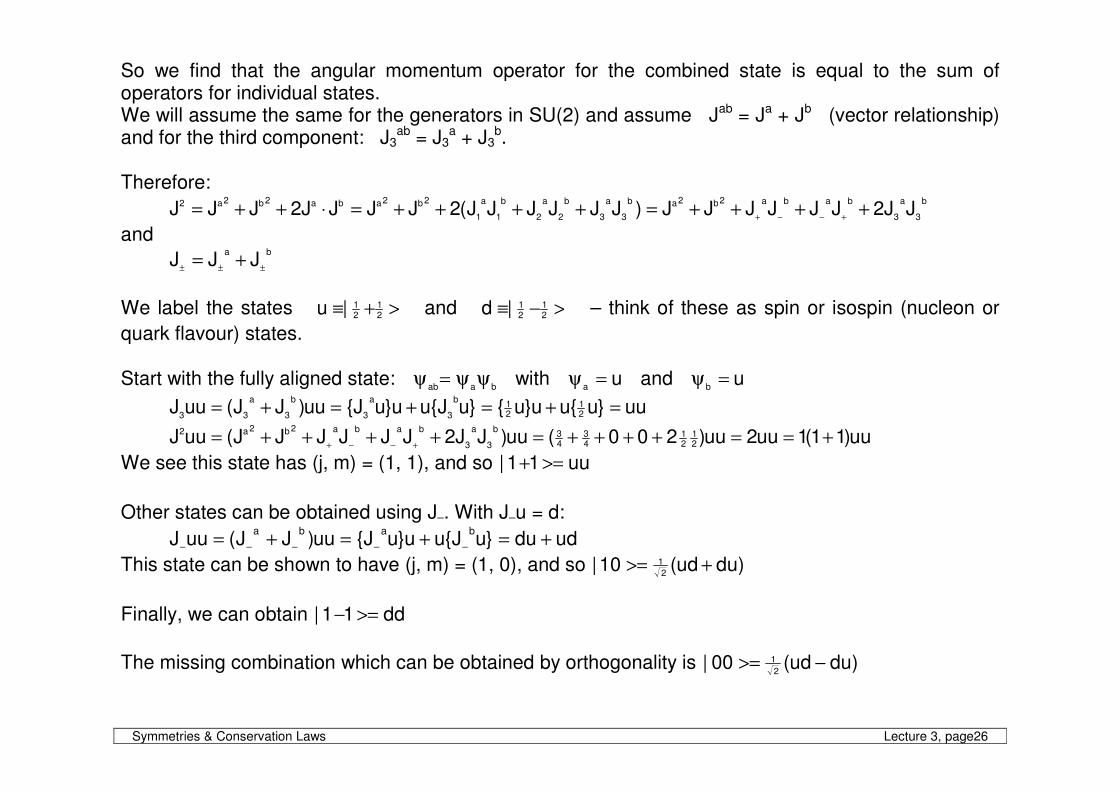
So we find that the angular momentum operator for the combined state is equal to the sum of operators for individual states. We will assume the same for the generators in SU(2) and assume Jab = Ja + Jb (vector relationship) and for the third component: J3
ab = J3a + J3
b. Therefore:
b
3
a
3
baba2b2ab
3
a
3
b
2
a
2
b
1
a
1
2b2aba2b2a2 JJ2JJJJJJ)JJJJJJ(2JJJJ2JJJ ++++=++++=⋅++=+−−+
and ba
JJJ±±±
+=
We label the states >+≡ 2
121|u and >−≡ 2
121|d – think of these as spin or isospin (nucleon or
quark flavour) states. Start with the fully aligned state:
baabψψ=ψ with u
a=ψ and u
b=ψ
uu}u{uu}u{}uJ{uu}uJ{uu)JJ(uuJ 21
21
b
3
a
3
b
3
a
33=+=+=+=
uu)11(1uu2uu)200(uu)JJ2JJJJJJ(uuJ 21
21
43
43
b
3
a
3
baba2b2a2 +==++++=++++=+−−+
We see this state has (j, m) = (1, 1), and so uu11| >=+
Other states can be obtained using J−. With J−u = d:
uddu}uJ{uu}uJ{uu)JJ(uuJbaba
+=+=+= −−−−−
This state can be shown to have (j, m) = (1, 0), and so )duud(10|2
1 +>=
Finally, we can obtain dd11| >=−
The missing combination which can be obtained by orthogonality is )duud(00|
2
1 −>=
Symmetries & Conservation Laws Lecture 3, page27
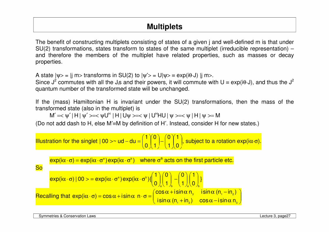
Multiplets The benefit of constructing multiplets consisting of states of a given j and well-defined m is that under SU(2) transformations, states transform to states of the same multiplet (irreducible representation) – and therefore the members of the multiplet have related properties, such as masses or decay properties.
A state |ψ> = |j m> transforms in SU(2) to |ψ′> = U|ψ> ≡ exp(iθ⋅J) |j m>.
Since J2 commutes with all the Jis and their powers, it will commute with U ≡ exp(iθ⋅J), and thus the J2 quantum number of the transformed state will be unchanged. If the (mass) Hamiltonian H is invariant under the SU(2) transformations, then the mass of the transformed state (also in the multiplet) is
M|H||HUU|U|H|U|H|M HH >=ψψ>=<ψψ>=<ψψ>=<ψ′ψ′=<′
(Do not add dash to H, else M′≡M by definition of H′. Instead, consider H for new states.)
Illustration for the singlet
−
=−>
0
1
1
0
1
0
0
1duud~00| , subject to a rotation exp(iα⋅σ).
)iexp()iexp()iexp( ba σ⋅ασ⋅α=σ⋅α where σa acts on the first particle etc.
So
}0
1
1
0
1
0
0
1){iexp()iexp(00|)iexp(
baba
ba
−
σ⋅ασ⋅α=>σ⋅α
Recalling that
α−α+α
−αα+α=σ⋅α+α=σ⋅α
321
213
nsinicos)inn(sini
)inn(sininsinicosnsinicos)iexp(
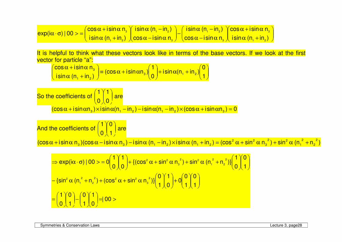
Symmetries & Conservation Laws Lecture 3, page28
+α
α+α
α−α
−α−
α−α
−α
+α
α+α=>σ⋅α
)inn(sini
nsinicos
nsinicos
)inn(sini
nsinicos
)inn(sini
)inn(sini
nsinicos00|)iexp(
21
3
3
21
3
21
21
3
It is helpful to think what these vectors look like in terms of the base vectors. If we look at the first vector for particle “a”:
+α+
α+α≡
+α
α+α
1
0)inn(sini
0
1)nsini(cos
)inn(sini
nsinicos213
21
3
So the coefficients of
0
1
0
1 are
0)nsini(cos)inn(sini)inn(sini)nsini(cos 321213 =α+α×−α−−α×α+α
And the coefficients of
1
0
0
1 are
)nn(sin)nsin(cos)inn(sini)inn(sini)nsini)(cosnsini(cos2
2
2
1
22
3
22
212133 +α+α+α=+α×−α−α−αα+α
>=
−
=
+
α+α++α−
+α+α+α+
=>σ⋅α⇒
00|0
1
1
0
1
0
0
1
1
0
1
00
0
1
1
0)}nsin(cos)nn({sin
1
0
0
1)}nn(sin)nsin{(cos
0
1
0
1000|)iexp(
2
3
222
2
2
1
2
2
2
2
1
22
3
22
Symmetries & Conservation Laws Lecture 3, page29
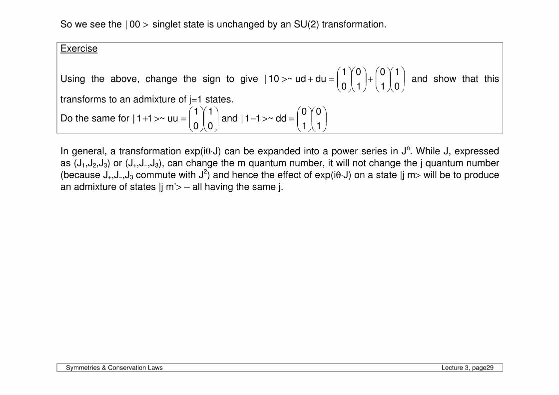
So we see the >00| singlet state is unchanged by an SU(2) transformation.
Exercise
Using the above, change the sign to give
+
=+>
0
1
1
0
1
0
0
1duud~10| and show that this
transforms to an admixture of j=1 states.
Do the same for
=>+
0
1
0
1uu~11| and
=>−
1
0
1
0dd~11|
In general, a transformation exp(iθ⋅J) can be expanded into a power series in Jn. While J, expressed
as (J1,J2,J3) or (J+,J−,J3), can change the m quantum number, it will not change the j quantum number
(because J+,J−,J3 commute with J2) and hence the effect of exp(iθ⋅J) on a state |j m> will be to produce
an admixture of states |j m’> – all having the same j.
Symmetries & Conservation Laws Lecture 3, page30
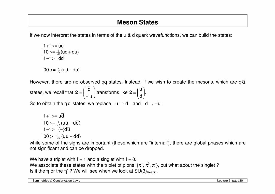
Meson States If we now interpret the states in terms of the u & d quark wavefunctions, we can build the states:
uu11| >=+
)duud(10|2
1 +>=
dd11| >=−
)duud(00|
2
1 −>=
However, there are no observed qq states. Instead, if we wish to create the mesons, which are q q
states, we recall that
−=
u
d2 transforms like
≡
d
u2 .
So to obtain the q q states, we replace du → and ud −→ :
du11| >=+
)dduu(10|2
1 −>=
ud)(11| −>=−
)dduu(00|2
1 +>=
while some of the signs are important (those which are “internal”), there are global phases which are not significant and can be dropped. We have a triplet with I = 1 and a singlet with I = 0.
We associate these states with the triplet of pions: {π+, π0, π−}, but what about the singlet ?
Is it the η or the η’ ? We will see when we look at SU(3)Isospin.
Symmetries & Conservation Laws Lecture 3, page31
Weights [6.1, 6.3, 6.4] We want to find the set of commuting Hermitian operators for a given system, since these correspond to the independent, simultaneous observables. The set of commuting generators is called the Cartan Subalgebra. The associated eigenvalues are the Weights. Weight Vectors are constructed from the eigenvalues from all of the commuting generators for a given label of the base vector. (The weights of the adjoint representation are called the Roots – they are related to the raising and lowering operators.)
In SU(2), the simplest representation is in terms of the (22−1)=3 2×2 σ matrices.
There is 1 commuting operator, J3, giving rise to 2 weight vectors, (m=−½) and (m=+½) – these are just points on a line.
In SU(3), the simplest representation is in terms of the (32−1)=8 3×3 λ matrices.
There are 2 commuting operators, λ3 and λ8, giving rise to 3 weight vectors, of the form (m,Y) – these are points in a plane. The weights are useful for classifying states and combinations of states.
Symmetries & Conservation Laws Lecture 3, page32
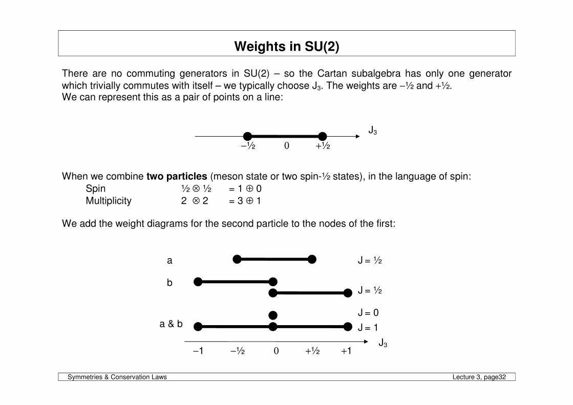
Weights in SU(2) There are no commuting generators in SU(2) – so the Cartan subalgebra has only one generator
which trivially commutes with itself – we typically choose J3. The weights are −½ and +½. We can represent this as a pair of points on a line:
When we combine two particles (meson state or two spin-½ states), in the language of spin:
Spin ½ ⊗ ½ = 1 ⊕ 0
Multiplicity 2 ⊗ 2 = 3 ⊕ 1 We add the weight diagrams for the second particle to the nodes of the first:
J = 0
−½ +½ 0 +1 −1 J3
a
b
a & b J = 1
J = ½
J = ½
J3
−½ +½ 0
Symmetries & Conservation Laws Lecture 3, page33
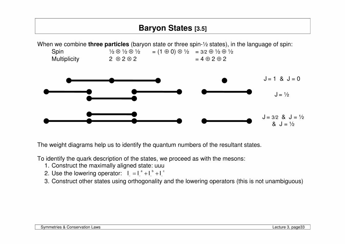
Baryon States [3.5] When we combine three particles (baryon state or three spin-½ states), in the language of spin:
Spin ½ ⊗ ½ ⊗ ½ = (1 ⊕ 0) ⊗ ½ = 3/2 ⊕ ½ ⊕ ½
Multiplicity 2 ⊗ 2 ⊗ 2 = 4 ⊕ 2 ⊕ 2
The weight diagrams help us to identify the quantum numbers of the resultant states. To identify the quark description of the states, we proceed as with the mesons:
1. Construct the maximally aligned state: uuu
2. Use the lowering operator: cba
IIII−−−−
++=
3. Construct other states using orthogonality and the lowering operators (this is not unambiguous)
J = 1 & J = 0
J = ½
J = 3/2 & J = ½ & J = ½
Symmetries & Conservation Laws Lecture 3, page34
We can create states:
I = 3/2 (= 1 + ½) Symmetric in 1 ↔ 2 ↔ 3
I3 = +3/2 uuu
I3 = +½ )duuuduuud(3
1 ++
I3 = −½ )ddudududd(3
1 ++
I3 = −3/2 ddd
I = ½ (= 1 − ½) Symmetric in 1 ↔ 2
I3 = +½ )2
duuuduuud(3
2+
−
I3 = −½ )2
udddudddu(3
2+
−
I = ½ (= 0 + ½) Asymmetric in 1 ↔ 2
I3 = +½ u)duud(2
1 −
I3 = −½ d)uddu(2
1 −
We can identify the I = 3/2 multiplet as the particles: ( −+++ ∆∆∆∆ ,,, 0 )
Which states correspond to (p, n), since there are two I = ½ multiplets ? Exercise
Show that the effect of the lowering operator on the state (I=½, I3=+½) is to produce the state
(I=½, I3=−½).
Symmetries & Conservation Laws Lecture 3, page35
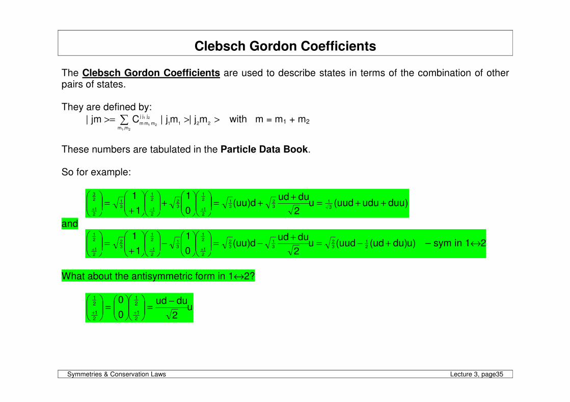
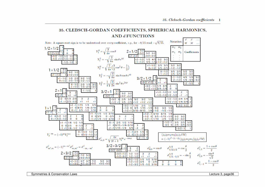
Clebsch Gordon Coefficients The Clebsch Gordon Coefficients are used to describe states in terms of the combination of other pairs of states. They are defined by:
>>>= ∑ 2211m,m
jjj
mmmmj|mj|Cjm|
21
21
21 with m = m1 + m2
These numbers are tabulated in the Particle Data Book. So for example:
)duuuduuud(u2
duudd)uu(
0
1
1
13
132
31
21
21
32
21
21
31
21
23
++=+
+=
+
+=
+−+
and
)u)duud(uud(u2
duudd)uu(
0
1
1
121
32
31
32
21
21
31
21
21
32
21
21
+−=+
−=
−
+=
+−+
– sym in 1↔2
What about the antisymmetric form in 1↔2?
u2
duud
0
0
21
21
21
21 −
=
=
++
Symmetries & Conservation Laws Lecture 3, page36