LECTURE 3: Fluid Statics

We begin by considering static fluid configurations, for which the stress tensor reduces to theform T = −pI, so that n ·T · n = −p, and the normal stress balance assumes the form:

p− p = σ ∇ · n (1)

The pressure jump across the interface is balanced by the curvature force at the interface. Nowsince n ·T ·s = 0 for a static system , the tangential stress balance equation indicates that: 0 = ∇σ.This leads us to the following important conclusion:

There cannot be a static system in the presence of surface tension gradients. While pressure jumpscan sustain normal stress jumps across a fluid interface, they do not contribute to the tangentialstress jump. Consequently, tangential surface stresses can only be balanced by viscous stressesassociated with fluid motion.

We proceed by applying equation (1) to a number of static situations.

3.1 Stationary bubble

We consider a spherical bubble of radius R submerged in a static fluid. What is the pressure dropacross the bubble surface?

The curvature of the spherical surface is simply computed:

∇ · n = ∇ · r =1r2

∂

∂r(r2) =

2R

(2)

so the normal stress jump (1) indicates that

p− p =2σ

R. (3)

The pressure within the bubble is higher than that outside by an amount proportional to thesurface tension, and inversely proportional to the bubble size. It is thus that small bubbles arelouder than large ones when they burst at a free surface: champagne is louder than beer. We notethat soap bubbles in air have two surfaces that define the inner and outer surfaces of the soap film;consequently, the pressure differential is twice that across a single interface.

3.2 Static meniscus

Consider a situation where the pressure within a static fluid varies owing to the presence of agravitational field, p = p0 + ρgz, where p0 is the constant ambient pressure, and ~g = −gz is thegravitational acceleration. The normal stress balance thus requires that the interface satisfy theYoung-Laplace Equation:

ρgz = σ ∇ · n . (4)

The vertical gradient in fluid pressure must be balanced by the curvature pressure; as the gradientis constant, the curvature must likewise increase linearly with z. Such a situation arises in thestatic meniscus (see Figure 1).

The shape of the meniscus is prescribed by two factors: the contact angle between the air-waterinterface and the log, and the balance between hydrostatic pressure and curvature pressure. We

1

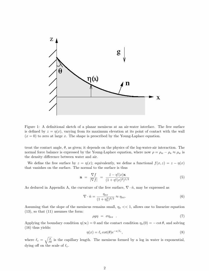
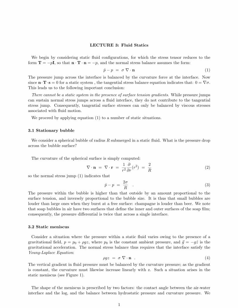
Figure 1: A definitional sketch of a planar meniscus at an air-water interface. The free surfaceis defined by z = η(x), varying from its maximum elevation at its point of contact with the wall(x = 0) to zero at large x. The shape is prescribed by the Young-Laplace equation.

treat the contact angle, θ, as given; it depends on the physics of the log-water-air interaction. Thenormal force balance is expressed by the Young-Laplace equation, where now ρ = ρw − ρa ≈ ρw isthe density difference between water and air.

We define the free surface by z = η(x); equivalently, we define a functional f(x, z) = z − η(x)that vanishes on the surface. The normal to the surface is thus

n =∇f

|∇f |=

z − η′(x)x(1 + η′(x)2)1/2

(5)

As deduced in Appendix A, the curvature of the free surface, ∇ · n, may be expressed as

∇ · n =ηxx

(1 + η2x)3/2

≈ ηxx. (6)

Assuming that the slope of the meniscus remains small, ηx << 1, allows one to linearize equation(13), so that (11) assumes the form:

ρgη = σηxx . (7)

Applying the boundary condition η(∞) = 0 and the contact condition ηx(0) = − cot θ, and solving(16) thus yields:

η(x) = `c cot(θ)e−x/`c , (8)

where `c =√

σρg is the capillary length. The meniscus formed by a log in water is exponential,

dying off on the scale of `c.

2

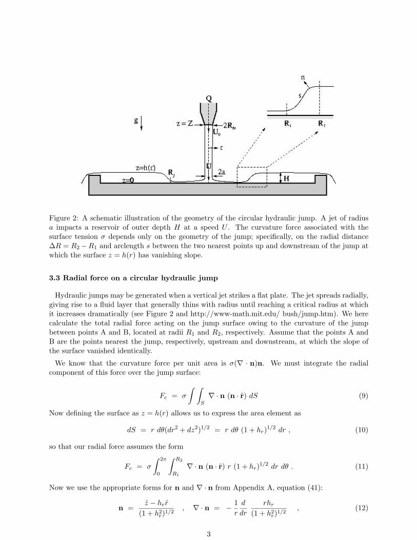
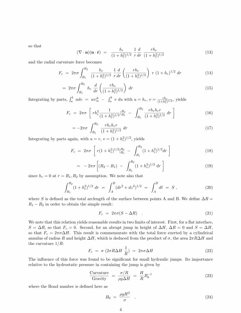
Figure 2: A schematic illustration of the geometry of the circular hydraulic jump. A jet of radiusa impacts a reservoir of outer depth H at a speed U . The curvature force associated with thesurface tension σ depends only on the geometry of the jump; specifically, on the radial distance∆R = R2−R1 and arclength s between the two nearest points up and downstream of the jump atwhich the surface z = h(r) has vanishing slope.

3.3 Radial force on a circular hydraulic jump

Hydraulic jumps may be generated when a vertical jet strikes a flat plate. The jet spreads radially,giving rise to a fluid layer that generally thins with radius until reaching a critical radius at whichit increases dramatically (see Figure 2 and http://www-math.mit.edu/ bush/jump.htm). We herecalculate the total radial force acting on the jump surface owing to the curvature of the jumpbetween points A and B, located at radii R1 and R2, respectively. Assume that the points A andB are the points nearest the jump, respectively, upstream and downstream, at which the slope ofthe surface vanished identically.

We know that the curvature force per unit area is σ(∇ · n)n. We must integrate the radialcomponent of this force over the jump surface:

Fc = σ

∫ ∫S∇ · n (n · r) dS (9)

Now defining the surface as z = h(r) allows us to express the area element as

dS = r dθ(dr2 + dz2)1/2 = r dθ (1 + hr)1/2 dr , (10)

so that our radial force assumes the form

Fc = σ

∫ 2π

0

∫ R2

R1

∇ · n (n · r) r (1 + hr)1/2 dr dθ . (11)

Now we use the appropriate forms for n and ∇ · n from Appendix A, equation (41):

n =z − hrr

(1 + h2r)1/2

, ∇ · n = − 1r

d

dr

rhr

(1 + h2r)1/2

, (12)

3

so that(∇ · n)(n · r) =

hr

(1 + h2r)1/2

1r

d

dr

rhr

(1 + h2r)1/2

(13)

and the radial curvature force becomes

Fc = 2πσ

∫ R2

R1

hr

(1 + h2r)1/2

1r

d

dr

(rhr

(1 + h2r)1/2

)r (1 + hr)1/2 dr (14)

= 2πσ

∫ R2

R1

hrd

dr

(rhr

(1 + h2r)1/2

)dr (15)

Integrating by parts,∫ ba udv = uv|ba −

∫ ba v du with u = hr, v = rhr

(1+h2r)1/2 , yields

Fc = 2πσ

[rh2

r

1(1 + h2

r)1/2|R2R1

−∫ R2

R1

rhrhrr

(1 + h2r)1/2

dr

](16)

= −2πσ

∫ R2

R1

rhrhrr

(1 + h2r)1/2

dr (17)

Integrating by parts again, with u = r, v = (1 + h2r)

1/2, yields

Fc = 2πσ

[r(1 + h2

r)1/2|R2

R1−

∫ R2

R1

(1 + h2r)

1/2dr

](18)

= − 2πσ

[(R2 −R1) −

∫ R2

R1

(1 + h2r)

1/2 dr

](19)

since hr = 0 at r = R1, R2 by assumption. We note also that∫ R2

R1

(1 + h2r)

1/2 dr =∫ B

A(dr2 + dz2)1/2 =

∫ B

Ad` = S , (20)

where S is defined as the total arclength of the surface between points A and B. We define ∆R =R1 −R2 in order to obtain the simple result:

Fc = 2πσ(S −∆R) . (21)

We note that this relation yields reasonable results in two limits of interest. First, for a flat interface,S = ∆R, so that Fc = 0. Second, for an abrupt jump in height of ∆H, ∆R = 0 and S = ∆H,so that Fc = 2πσ∆H. This result is commensurate with the total force exerted by a cylindricalannulus of radius R and height ∆H, which is deduced from the product of σ, the area 2πR∆H andthe curvature 1/R:

Fc = σ (2πR∆H1R

) = 2πσ∆H (22)

The influence of this force was found to be significant for small hydraulic jumps. Its importancerelative to the hydrostatic pressure in containing the jump is given by

CurvatureGravity

=σ/R

ρg∆H=

H

RB−1

0 (23)

where the Bond number is defined here as

B0 =ρgH2

σ. (24)

4

The simple result (19) was derived by Bush & Aristoff (2003), who also presented the results ofan experimental study of circular hydraulic jumps. Their experiments indicated that the curvatureforce becomes appreciable for jumps with characteristic radius of less than 3 cm.

While the influence of surface tension on the radius of the circular hydraulic jump is generallysmall, it may have a qualitative influence on the shape of the jump. In particular, it may prompt theaxisymmetry-breaking instability responsible for the polygonal hydraulic jump structures discoveredby Elegaard et al. (Nature, 1998), and more recently examined by Bush, Hosoi & Aristoff (2004).See http://www-math.mit.edu/ bush/jump.htm.

3.4 Floating Bodies

Floating bodies must be supported by some combination of buoyancy and curvature forces. Specif-ically, since the fluid pressure beneath the interface is related to the atmospheric pressure P0 abovethe interface by

p = P0 + ρgz + σ∇ · n ,

one may express the vertical force balance as

Mg = z ·∫

c−p n d` = Fb + Fc . (25)

The buoyancy force

Fb = z ·∫

Cρgz n d` = ρgVb (26)

is thus sim

bove the object and inside the line of tangency (Figure 3). A simple expression for the curvatureforce may be deduced using the first of the Frenet-Serret equations (see Appendix B).

Fc = z ·∫

Cσ(∇ · n)n d` = σz ·

∫C

dtd`

d` = σz · (t1 − t2) = 2σ sinθ (27)

At the interface, the buoyancy and curvature forces must balance precisely, so the Young-Laplacerelation is satisfied:

0 = ρgz + σ∇ · n (28)

Integrating the fluid pressure over the meniscus yields the vertical force balance:

Fmb + Fm

c = 0 . (29)

where

Fmb = z ·

∫Cm

ρgzn d` = ρgVm (30)

5

CL VmV

θ

b

m

C

air

water

t t

t1

t2

x x

r

g

n

C

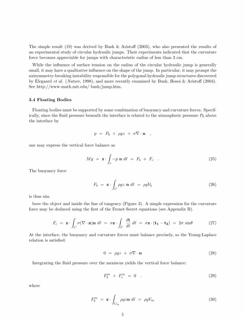
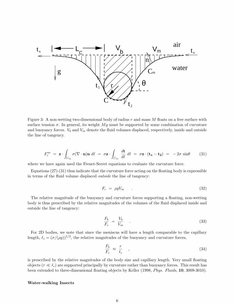
Figure 3: A non-wetting two-dimensional body of radius r and mass M floats on a free surface withsurface tension σ. In general, its weight Mg must be supported by some combination of curvatureand buoyancy forces. Vb and Vm denote the fluid volumes displaced, respectively, inside and outsidethe line of tangency.

Fmc = z ·

∫Cm

σ(∇ · n)n d` = σz ·∫

Cm

dtd`

d` = σz · (tx − t2) = − 2σ sinθ (31)

where we have again used the Frenet-Serret equations to evaluate the curvature force.

Equations (27)-(31) thus indicate that the curvature force acting on the floating body is expressiblein terms of the fluid volume displaced outside the line of tangency:

Fc = ρgVm . (32)

The relative magnitude of the buoyancy and curvature forces supporting a floating, non-wettingbody is thus prescribed by the relative magnitudes of the volumes of the fluid displaced inside andoutside the line of tangency:

Fb

Fc=

Vb

Vm. (33)

For 2D bodies, we note that since the meniscus will have a length comparable to the capillarylength, `c = (σ/(ρg))1/2, the relative magnitudes of the buoyancy and curvature forces,

Fb

Fc≈ r

`c, (34)

is prescribed by the relative magnitudes of the body size and capillary length. Very small floatingobjects (r � `c) are supported principally by curvature rather than buoyancy forces. This result hasbeen extended to three-dimensional floating objects by Keller (1998, Phys. Fluids, 10, 3009-3010).

Water-walking Insects

6

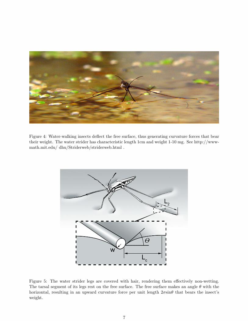
Figure 4: Water-walking insects deflect the free surface, thus generating curvature forces that beartheir weight. The water strider has characteristic length 1cm and weight 1-10 mg. See http://www-math.mit.edu/ dhu/Striderweb/striderweb.html .

Figure 5: The water strider legs are covered with hair, rendering them effectively non-wetting.The tarsal segment of its legs rest on the free surface. The free surface makes an angle θ with thehorizontal, resulting in an upward curvature force per unit length 2σsinθ that bears the insect’sweight.

7

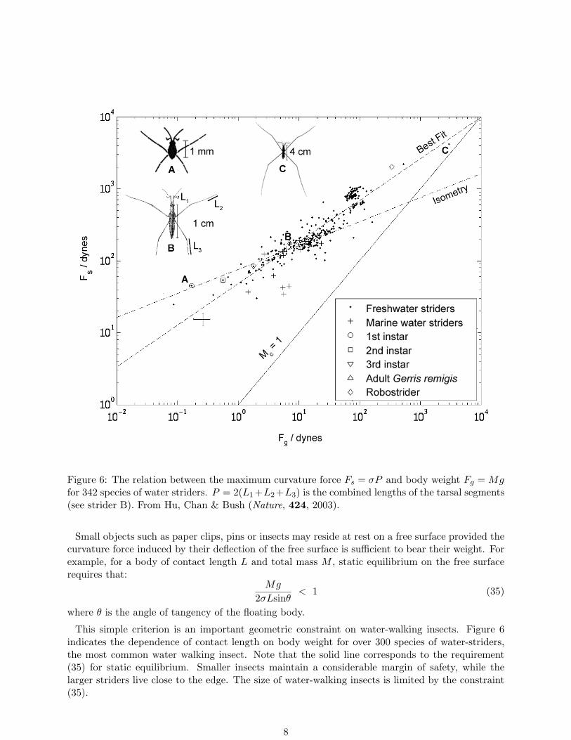
Figure 6: The relation between the maximum curvature force Fs = σP and body weight Fg = Mgfor 342 species of water striders. P = 2(L1+L2+L3) is the combined lengths of the tarsal segments(see strider B). From Hu, Chan & Bush (Nature, 424, 2003).

Small objects such as paper clips, pins or insects may reside at rest on a free surface provided thecurvature force induced by their deflection of the free surface is sufficient to bear their weight. Forexample, for a body of contact length L and total mass M , static equilibrium on the free surfacerequires that:

Mg

2σLsinθ< 1 (35)

where θ is the angle of tangency of the floating body.

This simple criterion is an important geometric constraint on water-walking insects. Figure 6indicates the dependence of contact length on body weight for over 300 species of water-striders,the most common water walking insect. Note that the solid line corresponds to the requirement(35) for static equilibrium. Smaller insects maintain a considerable margin of safety, while thelarger striders live close to the edge. The size of water-walking insects is limited by the constraint(35).

8

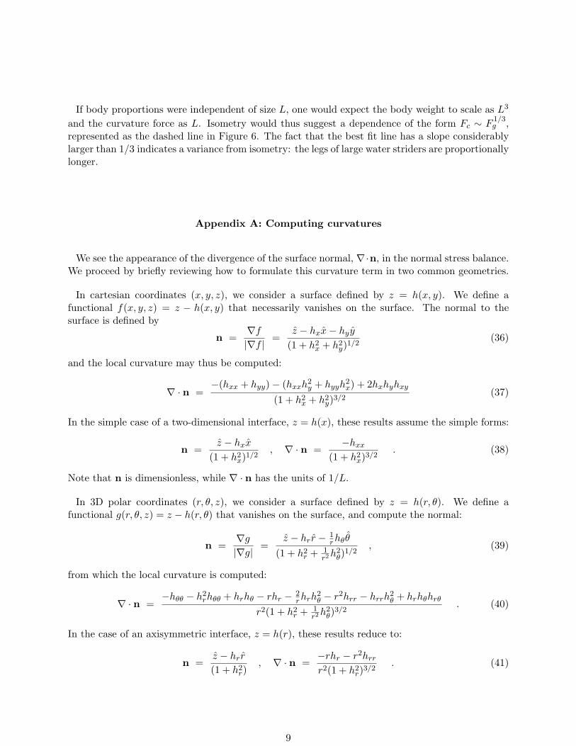
If body proportions were independent of size L, one would expect the body weight to scale as L3

and the curvature force as L. Isometry would thus suggest a dependence of the form Fc ∼ F1/3g ,

represented as the dashed line in Figure 6. The fact that the best fit line has a slope considerablylarger than 1/3 indicates a variance from isometry: the legs of large water striders are proportionallylonger.

Appendix A: Computing curvatures

We see the appearance of the divergence of the surface normal, ∇·n, in the normal stress balance.We proceed by briefly reviewing how to formulate this curvature term in two common geometries.

In cartesian coordinates (x, y, z), we consider a surface defined by z = h(x, y). We define afunctional f(x, y, z) = z − h(x, y) that necessarily vanishes on the surface. The normal to thesurface is defined by

n =∇f

|∇f |=

z − hxx− hyy

(1 + h2x + h2

y)1/2(36)

and the local curvature may thus be computed:

∇ · n =−(hxx + hyy)− (hxxh2

y + hyyh2x) + 2hxhyhxy

(1 + h2x + h2

y)3/2(37)

In the simple case of a two-dimensional interface, z = h(x), these results assume the simple forms:

n =z − hxx

(1 + h2x)1/2

, ∇ · n =−hxx

(1 + h2x)3/2

. (38)

Note that n is dimensionless, while ∇ · n has the units of 1/L.

In 3D polar coordinates (r, θ, z), we consider a surface defined by z = h(r, θ). We define afunctional g(r, θ, z) = z − h(r, θ) that vanishes on the surface, and compute the normal:

n =∇g

|∇g|=

z − hrr − 1rhθθ

(1 + h2r + 1

r2 h2θ)

1/2, (39)

from which the local curvature is computed:

∇ · n =−hθθ − h2

rhθθ + hrhθ − rhr − 2rhrh

2θ − r2hrr − hrrh

2θ + hrhθhrθ

r2(1 + h2r + 1

r2 h2θ)

3/2. (40)

In the case of an axisymmetric interface, z = h(r), these results reduce to:

n =z − hrr

(1 + h2r)

, ∇ · n =−rhr − r2hrr

r2(1 + h2r)3/2

. (41)

9

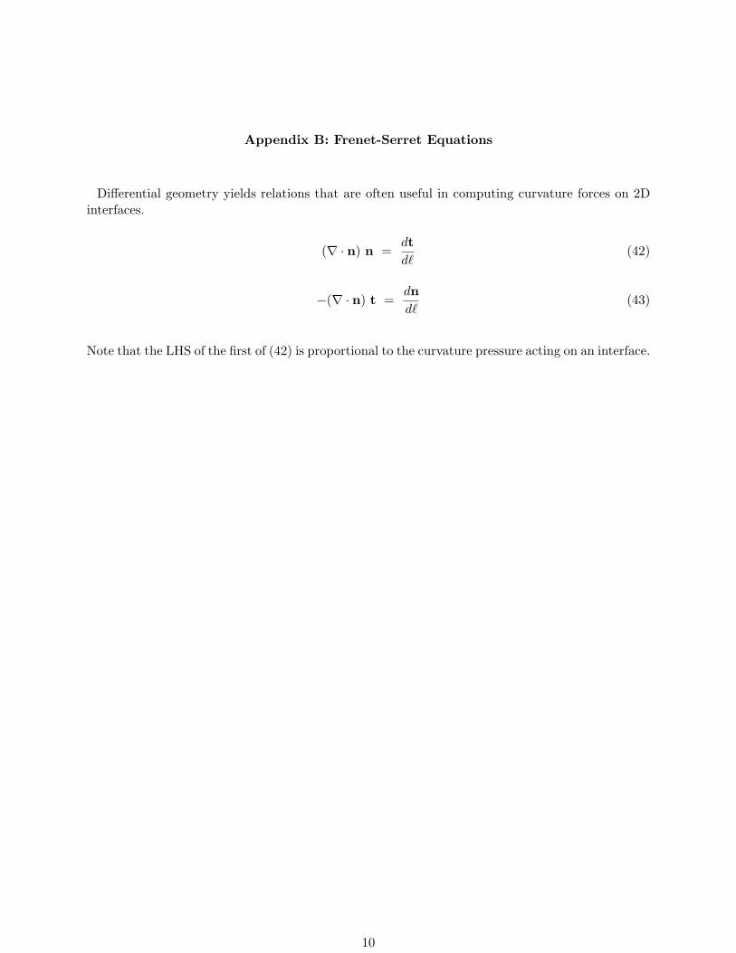
Appendix B: Frenet-Serret Equations

Differential geometry yields relations that are often useful in computing curvature forces on 2Dinterfaces.

(∇ · n) n =dtd`

(42)

−(∇ · n) t =dnd`

(43)

Note that the LHS of the first of (42) is proportional to the curvature pressure acting on an interface.

10