Geometric Numerical Integration TU MunchenErnst Hairer January – February 2010

Lecture 3: Backward error analysisTable of contents

1 Modified differential equation 12 Modified Hamiltonian for symplectic integrators 53 Near conservation of the total energy 64 Counter-example: Takahashi–Imada integrator 105 Existence of global modified Hamiltonian 136 Completely integrable Hamiltonian systems 157 Linear error growth for integrable systems 178 Exercises 20

Backward error analysis is the most powerful tool for the study of the long-timebehaviour of numerical integrators.

1 Modified differential equation

��

��

�*

��

��

�*

HH

HH

Hj

��

���

��

���

HH

HHH

y = f(y)

ϕt(y0)

yn+1 = Φh(yn)

˙y = fh(y )

exact

numerical

exact

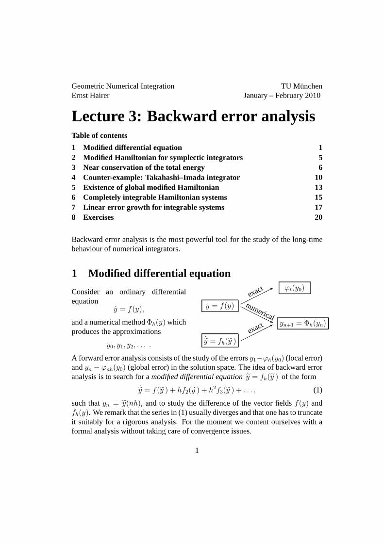
Consider an ordinary differentialequation

y = f(y),

and a numerical methodΦh(y) whichproduces the approximations

y0, y1, y2, . . . .

A forward error analysis consists of the study of the errorsy1−ϕh(y0) (local error)andyn − ϕnh(y0) (global error) in the solution space. The idea of backward erroranalysis is to search for amodified differential equationy = fh(y ) of the form

˙y = f(y ) + hf2(y ) + h2f3(y ) + . . . , (1)

such thatyn = y(nh), and to study the difference of the vector fieldsf(y) andfh(y). We remark that the series in (1) usually diverges and that one has to truncateit suitably for a rigorous analysis. For the moment we content ourselves with aformal analysis without taking care of convergence issues.

1

For the computation of the modified equation (1) we puty := y(t) for a fixedt,and we expand the solution of (1) into a Taylor series

y(t+ h) = y + h(f(y) + hf2(y) + h2f3(y) + . . .

)

+h2

2!

(f ′(y) + hf ′

2(y) + . . .)(f(y) + hf2(y) + . . .

)+ . . . .

(2)

We assume that the numerical methodΦh(y) can be expanded as

Φh(y) = y + hf(y) + h2d2(y) + h3d3(y) + . . . (3)

(the coefficient ofh is f(y) for consistent methods). The functionsdj(y) areknown and are typically composed off(y) and its derivatives. To gety(nh) = yn

for all n, we must havey(t + h) = Φh(y). Comparing like powers ofh in theexpressions (2) and (3) yields recurrence relations for thefunctionsfj(y):

f2(y) = d2(y) − 1

2!f ′f(y) (4)

f3(y) = d3(y) − 1

3!

(f ′′(f, f)(y) + f ′f ′f(y)

)− 1

2!

(f ′f2(y) + f ′

2f(y)).

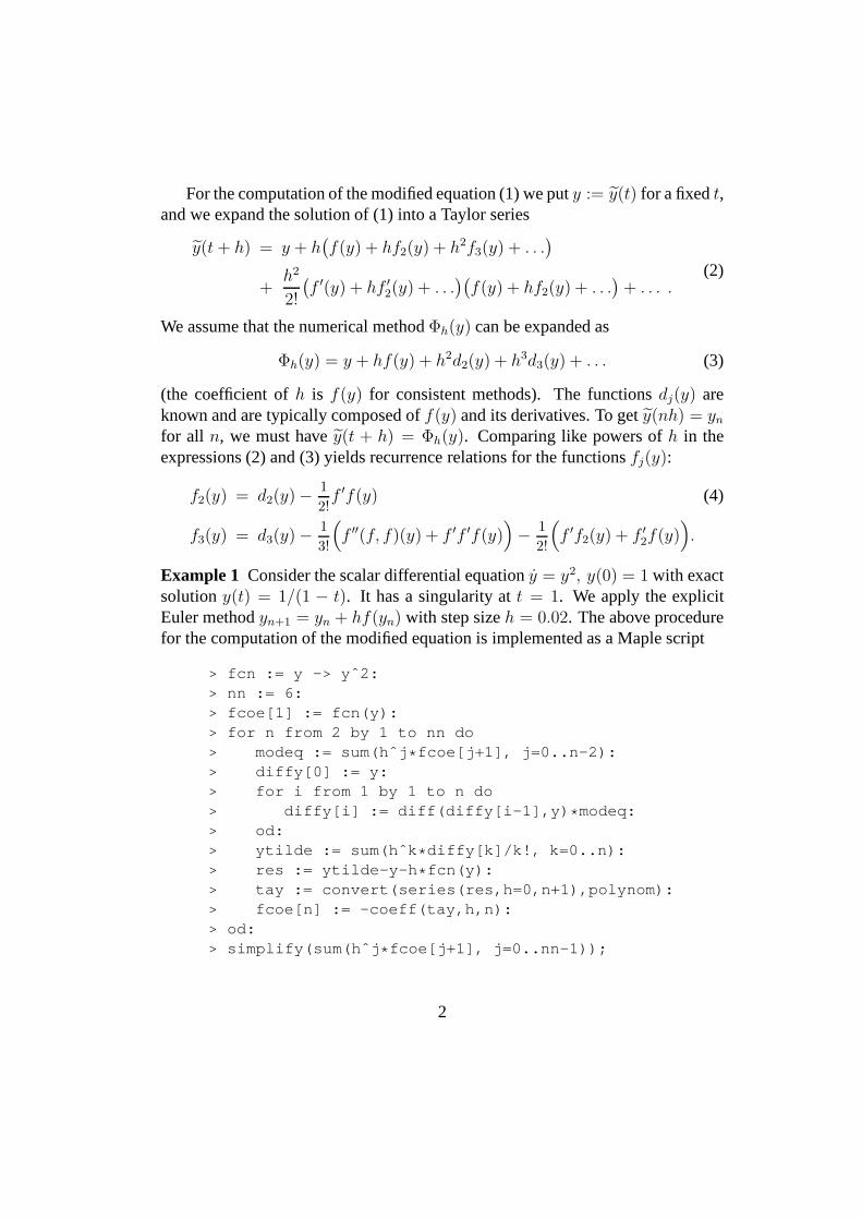
Example 1 Consider the scalar differential equationy = y2, y(0) = 1 with exactsolutiony(t) = 1/(1 − t). It has a singularity att = 1. We apply the explicitEuler methodyn+1 = yn + hf(yn) with step sizeh = 0.02. The above procedurefor the computation of the modified equation is implemented as a Maple script

> fcn := y -> yˆ2:> nn := 6:> fcoe[1] := fcn(y):> for n from 2 by 1 to nn do> modeq := sum(hˆj * fcoe[j+1], j=0..n-2):> diffy[0] := y:> for i from 1 by 1 to n do> diffy[i] := diff(diffy[i-1],y) * modeq:> od:> ytilde := sum(hˆk * diffy[k]/k!, k=0..n):> res := ytilde-y-h * fcn(y):> tay := convert(series(res,h=0,n+1),polynom):> fcoe[n] := -coeff(tay,h,n):> od:> simplify(sum(hˆj * fcoe[j+1], j=0..nn-1));

2

.6 .8 1.0

10

20exact solution

solutions of truncatedmodified equations

Figure 1: Solutions of the modified equation for the problemy = y2, y(0) = 1.

Its output is

˙y = y 2 − hy 3 + h2 3

2y 4 − h3 8

3y 5 + h4 31

6y 6 − h5 157

15y 7 ± . . . . (5)

Figure 1 presents the exact solution (dashed curve), the numerical solution (thickdots), and the solution of the modified equation, when truncated after 1, 2, 3, and4 terms. We observe an excellent agreement of the numerical solution with theexact solution of the modified equation.

A similar program for the implicit midpoint rule computes the modified equa-tion

˙y = y 2 + h2 1

4y 4 + h4 1

8y 6 + h6 11

192y 8 + h8 3

128y 10 ± . . . , (6)

and for the classical (explicit) Runge–Kutta method of order 4

˙y = y 2 − h4 1

24y 6 + h6 65

576y 8 − h7 17

96y 9 + h8 19

144y 10 ± . . . . (7)

We observe that the perturbation terms in the modified equation are of sizeO(hr), wherer is the order of the method. This is true in general.

Theorem 1 Suppose that the methodyn+1 = Φh(yn) is of orderr, i.e.,

Φh(y) = ϕh(y) + hr+1δr+1(y) + O(hr+2),

whereϕt(y) denotes the exact flow ofy = f(y), andhr+1δr+1(y) the leading termof the local truncation error. The modified equation then satisfies

˙y = f(y ) + hrfr+1(y ) + hr+1fr+2(y ) + . . . , y(0) = y0 (8)

with fr+1(y) = δr+1(y).

Proof. The construction of the functionsfj(y) (see the beginning of this section)shows thatfj(y) = 0 for 2 ≤ j ≤ r if and only if Φh(y) − ϕh(y) = O(hr+1).

3

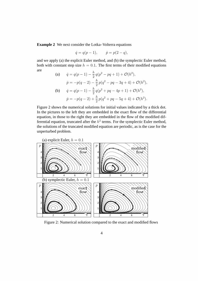
Example 2 We next consider the Lotka–Volterra equations

q = q(p− 1), p = p(2 − q),

and we apply (a) the explicit Euler method, and (b) the symplectic Euler method,both with constant step sizeh = 0.1. The first terms of their modified equationsare

(a) q = q(p− 1) − h

2q(p2 − pq + 1) + O(h2),

p = −p(q − 2) − h

2p(q2 − pq − 3q + 4) + O(h2),

(b) q = q(p− 1) − h

2q(p2 + pq − 4p+ 1) + O(h2),

p = −p(q − 2) +h

2p(q2 + pq − 5q + 4) + O(h2).

Figure 2 shows the numerical solutions for initial values indicated by a thick dot.In the pictures to the left they are embedded in the exact flow of the differentialequation, in those to the right they are embedded in the flow ofthe modified dif-ferential equation, truncated after theh2 terms. For the symplectic Euler method,the solutions of the truncated modified equation are periodic, as is the case for theunperturbed problem.

2 4 6

1

2

3

4

2 4 6

1

2

3

4

2 4 6

1

2

3

4

2 4 6

1

2

3

4

q

pexactflowexactflowexactflowexactflowexactflowexactflowexactflowexactflowexactflowexactflowexactflowexactflowexactflowexactflowexactflowexactflowexactflowexactflowexactflowexactflowexactflowexactflowexactflowexactflowexactflowexactflowexactflowexactflowexactflowexactflow

(a) explicit Euler,h = 0.1

q

pmodified

flowmodified

flowmodified

flowmodified

flowmodified

flowmodified

flowmodified

flowmodified

flowmodified

flowmodified

flowmodified

flowmodified

flowmodified

flowmodified

flowmodified

flowmodified

flowmodified

flowmodified

flowmodified

flowmodified

flowmodified

flowmodified

flowmodified

flowmodified

flowmodified

flowmodified

flowmodified

flowmodified

flowmodified

flowmodified

flow

q

pexactflowexactflowexactflowexactflowexactflowexactflowexactflowexactflowexactflowexactflowexactflowexactflowexactflowexactflowexactflowexactflowexactflowexactflowexactflowexactflowexactflowexactflowexactflowexactflowexactflowexactflowexactflowexactflowexactflowexactflow

(b) symplectic Euler,h = 0.1(b) symplectic Euler,h = 0.1

q

pmodified

flowmodified

flowmodified

flowmodified

flowmodified

flowmodified

flowmodified

flowmodified

flowmodified

flowmodified

flowmodified

flowmodified

flowmodified

flowmodified

flowmodified

flowmodified

flowmodified

flowmodified

flowmodified

flowmodified

flowmodified

flowmodified

flowmodified

flowmodified

flowmodified

flowmodified

flowmodified

flowmodified

flowmodified

flowmodified

flow

Figure 2: Numerical solution compared to the exact and modified flows

4

2 4 6

1

2

3

4

2 4 6

1

2

3

4

q

p Euler,h = 0.12

solutions ofmodifieddiff. equ.

q

p sympl. Euler,h = 0.12

solutions ofmodifieddiff. equ.

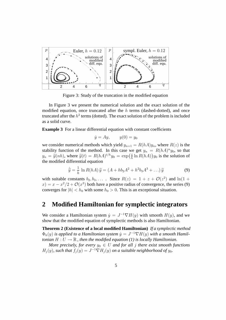
Figure 3: Study of the truncation in the modified equation

In Figure 3 we present the numerical solution and the exact solution of themodified equation, once truncated after theh terms (dashed-dotted), and oncetruncated after theh2 terms (dotted). The exact solution of the problem is includedas a solid curve.

Example 3 For a linear differential equation with constant coefficients

y = Ay, y(0) = y0

we consider numerical methods which yieldyn+1 = R(hA)yn, whereR(z) is thestability function of the method. In this case we getyn = R(hA)ny0, so thatyn = y(nh), wherey(t) = R(hA)t/hy0 = exp

(th

lnR(hA))y0 is the solution of

the modified differential equation

˙y =1

hlnR(hA) y = (A+ hb2A

2 + h2b3A3 + . . .) y (9)

with suitable constantsb2, b3, . . . . SinceR(z) = 1 + z + O(z2) and ln(1 +x) = x− x2/2 + O(x3) both have a positive radius of convergence, the series (9)converges for|h| < h0 with someh0 > 0. This is an exceptional situation.

2 Modified Hamiltonian for symplectic integrators

We consider a Hamiltonian systemy = J−1∇H(y) with smoothH(y), and weshow that the modified equation of symplectic methods is alsoHamiltonian.

Theorem 2 (Existence of a local modified Hamiltonian)If a symplectic methodΦh(y) is applied to a Hamiltonian systemy = J−1∇H(y) with a smooth Hamil-tonianH : U → R , then the modified equation (1) is locally Hamiltonian.

More precisely, for everyy0 ∈ U and for all j there exist smooth functionsHj(y), such thatfj(y) = J−1∇Hj(y) on a suitable neighborhood ofy0.

5

Proof.1 2 Assume thatfj(y) = J−1∇Hj(y) for j = 1, 2, . . . , r (this is satisfied forr = 1, becausef1(y) = f(y) = J−1∇H(y)). We have to prove the existence of aHamiltonianHr+1(y). The idea is to consider the truncated modified equation

˙y = f(y ) + hf2(y ) + . . .+ hr−1fr(y ), (10)

which is a Hamiltonian system with HamiltonianH(y)+hH2(y)+. . .+hr−1Hr(y).

Its flow ϕr,t(y0), compared to that of (1), satisfies

Φh(y0) = ϕr,h(y0) + hr+1fr+1(y0) + O(hr+2),

and alsoΦ′

h(y0) = ϕ′r,h(y0) + hr+1f ′

r+1(y0) + O(hr+2).

By our assumption on the method and by the induction hypothesis, Φh andϕr,h

are symplectic transformations. Together withϕ′r,h(y0) = I + O(h), this implies

J = Φ′h(y0)

TJΦ′h(y0) = J + hr+1

(f ′

r+1(y0)TJ + Jf ′

r+1(y0))

+ O(hr+2).

The matrixJf ′r+1(y) is therefore symmetric, and the (local) existence ofHr+1(y)

satisfyingfr+1(y) = J−1∇Hr+1(y) follows from the Integrability Lemma.

The application of the Integrability Lemma shows that the modified Hamilto-nian is globally defined onU , if U = R

2d, or if U is star-shaped, or ifU is simplyconnected.

3 Near conservation of the total energy

As a first application of backward error analysis we study thelong-time energyconservation of a symplectic numerical scheme (of orderr) applied to Hamilto-nian systemsy = J−1∇H(y). It follows from Theorem 2 that the correspondingmodified differential equation is also Hamiltonian. After truncation we get

H [N ](y) = H(y) + hrHr+1(y) + . . .+ hN−1HN(y), (11)

which we assume to beglobally defined on the same open set as the originalHamiltonianH(y).

1G. Benettin & A. Giorgilli,On the Hamiltonian interpolation of near to the identity symplecticmappings with application to symplectic integration algorithms, J. Statist. Phys. 74 (1994) 1117–1143.

2Y.-F. Tang,Formal energy of a symplectic scheme for Hamiltonian systems and its applica-tions (I), Computers Math. Applic. 27 (1994) 31–39.

6

Theorem 3 Consider a Hamiltonian system with smoothH : U → R (whereU ⊂ R

2d), apply a symplectic numerical methodΦh(y) with step sizeh, andassume that its modified Hamiltonian is globally defined onU .

If the numerical solution stays in the compact setK ⊂ U , then we have asymp-totically for h→ 0

H [N ](yn) = H [N ](y0) + O(t hN)

H(yn) = H(y0) + O(hr)

over time intervals of sizet = nh ≤ C h−N+r.

Proof. We letϕN,t(y0) be the flow of the truncated modified equation. The effectof the truncation is that‖yj+1 − ϕN,h(yj)‖ ≤ C hN+1. Since the truncated mod-ified equation is Hamiltonian withH [N ](y) of (11), we haveH [N ]

(ϕN,t(yj)

)=

H [N ](yj) for all times t. Using a globalh-independent Lipschitz constant forH [N ] on the compact setK, the statement on the long-time conservation ofH [N ]

is a consequence of

H [N ](yn) −H [N ](y0) =

n−1∑

j=0

(H [N ](yj+1) −H [N ](yj)

)

=

n−1∑

j=0

(H [N ](yj+1) −H [N ]

(ϕN,h(yj)

))= O(nhN+1).

The statement for the HamiltonianH follows from (11), becauseHr+1(y)+ . . .+hN−r−1HN(y) is uniformly bounded onK independently ofh andN .

If the Hamiltonian and the integrator are analytic, it is possible to prove expo-nentially small error bounds on exponentially large time intervals. More precisely,for sufficiently smallh there existsN = N(h) ∼ h−1 such that in the estimatesof the theorem abovehN can be replaced bye−γ/h.

Example 4 The mathematical pendulum is a system with one degree of freedomhaving the HamiltonianH(p, q) = 1

2p2 − cos q. Since the Hamiltonian and the

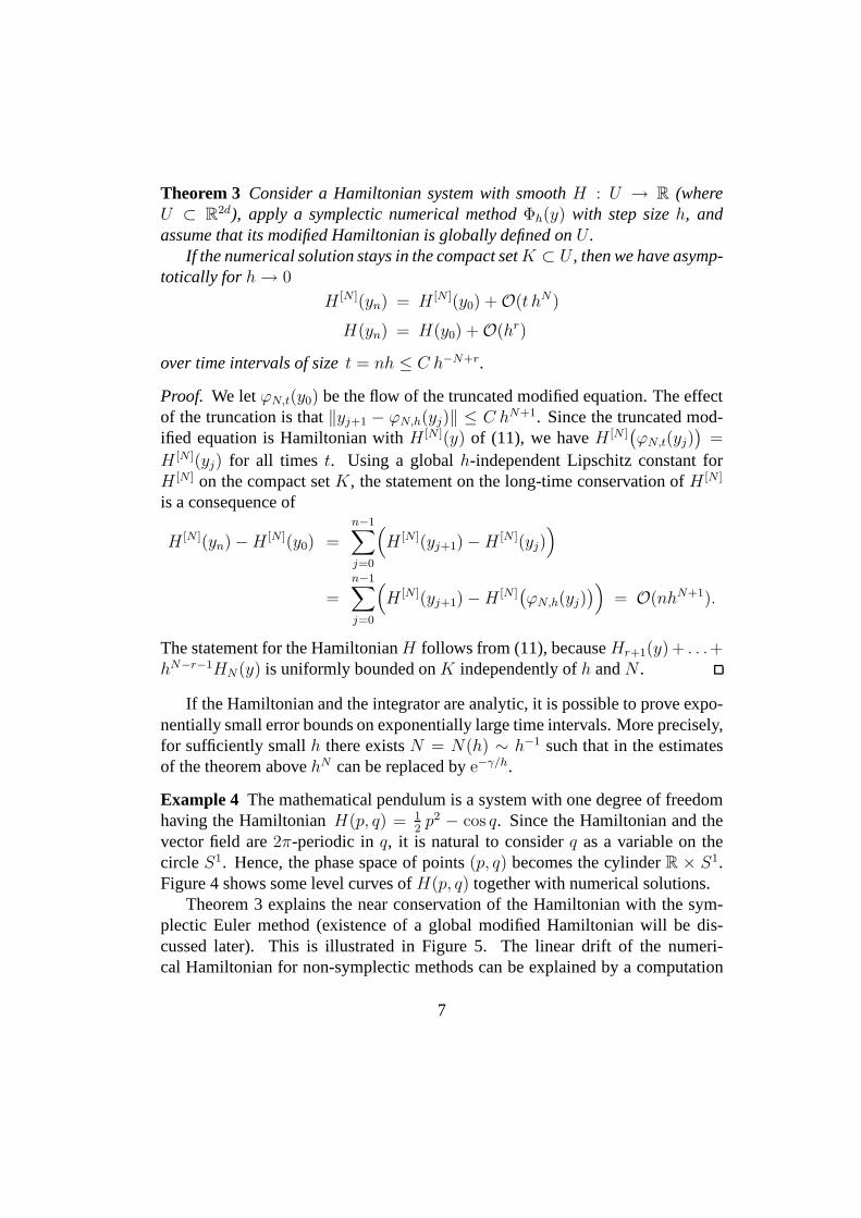
vector field are2π-periodic inq, it is natural to considerq as a variable on thecircleS1. Hence, the phase space of points(p, q) becomes the cylinderR × S1.Figure 4 shows some level curves ofH(p, q) together with numerical solutions.

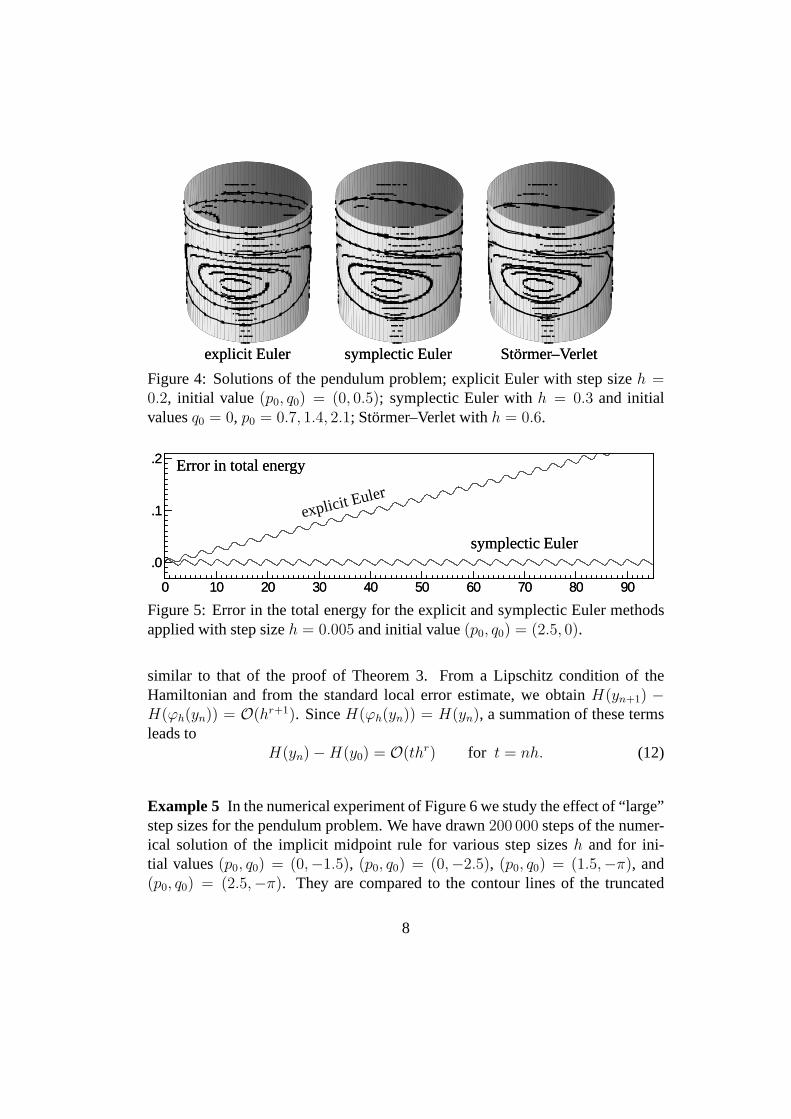
Theorem 3 explains the near conservation of the Hamiltonianwith the sym-plectic Euler method (existence of a global modified Hamiltonian will be dis-cussed later). This is illustrated in Figure 5. The linear drift of the numeri-cal Hamiltonian for non-symplectic methods can be explained by a computation

7

explicit Eulerexplicit Euler symplectic Eulersymplectic Euler Stormer–VerletStormer–Verlet

Figure 4: Solutions of the pendulum problem; explicit Eulerwith step sizeh =0.2, initial value (p0, q0) = (0, 0.5); symplectic Euler withh = 0.3 and initialvaluesq0 = 0, p0 = 0.7, 1.4, 2.1; Stormer–Verlet withh = 0.6.

0 10 20 30 40 50 60 70 80 90

.0

.1

.2

0 10 20 30 40 50 60 70 80 90

.0

.1

.2 Error in total energy

symplectic Euler

explicit Euler

Error in total energy

symplectic Euler

explicit Euler

Figure 5: Error in the total energy for the explicit and symplectic Euler methodsapplied with step sizeh = 0.005 and initial value(p0, q0) = (2.5, 0).

similar to that of the proof of Theorem 3. From a Lipschitz condition of theHamiltonian and from the standard local error estimate, we obtainH(yn+1) −H(ϕh(yn)) = O(hr+1). SinceH(ϕh(yn)) = H(yn), a summation of these termsleads to

H(yn) −H(y0) = O(thr) for t = nh. (12)

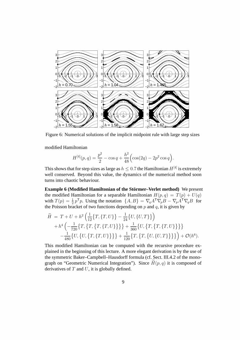
Example 5 In the numerical experiment of Figure 6 we study the effect of“large”step sizes for the pendulum problem. We have drawn200 000 steps of the numer-ical solution of the implicit midpoint rule for various stepsizesh and for ini-tial values(p0, q0) = (0,−1.5), (p0, q0) = (0,−2.5), (p0, q0) = (1.5,−π), and(p0, q0) = (2.5,−π). They are compared to the contour lines of the truncated

8

−3 −2 −1 0 1 2 3

−2

−1

0

1

2

3

h = 0.70h = 0.70

−3 −2 −1 0 1 2 3

−2

−1

0

1

2

3

h = 1.04h = 1.04

−3 −2 −1 0 1 2 3

−2

−1

0

1

2

3

h = 1.465h = 1.465

−3 −2 −1 0 1 2 3

−2

−1

0

1

2

3

h = 1.55h = 1.55

−3 −2 −1 0 1 2 3

−2

−1

0

1

2

3

h = 1.58h = 1.58

−3 −2 −1 0 1 2 3

−2

−1

0

1

2

3

h = 1.62h = 1.62

Figure 6: Numerical solutions of the implicit midpoint rulewith large step sizes

modified Hamiltonian

H [4](p, q) =p2

2− cos q +

h2

48

(cos(2q) − 2p2 cos q

).

This shows that for step sizes as large ash ≤ 0.7 the HamiltonianH [4] is extremelywell conserved. Beyond this value, the dynamics of the numerical method soonturns into chaotic behaviour.

Example 6 (Modified Hamiltonian of the Stormer–Verlet method) We presentthe modified Hamiltonian for a separable HamiltonianH(p, q) = T (p) + U(q)with T (p) = 1

2pTp. Using the notation{A,B} = ∇qA

T∇pB − ∇pAT∇qB for

the Poisson bracket of two functions depending onp andq, it is given by

H = T + U + h2(

1

12

{T, {T, U}

}− 1

24

{U, {U, T}

})

+h4(− 1

720

{T,

{T,

{T, {T, U}

}}}+

1

360

{U,

{T,

{T, {T, U}

}}}

− 1

480

{U,

{U,

{T, {T, U}

}}}+

1

120

{T,

{T,

{U, {U, T}

}}})+ O(h6).

This modified Hamiltonian can be computed with the recursiveprocedure ex-plained in the beginning of this lecture. A more elegant derivation is by the use ofthe symmetric Baker–Campbell–Hausdorff formula (cf. Sect. III.4.2 of the mono-graph on “Geometric Numerical Integration”). SinceH(p, q) it is composed ofderivatives ofT andU , it is globally defined.

9

4 Counter-example: Takahashi–Imada integrator

We consider a second order differential equationq = f(q), and we assume thatit is Hamiltonian, i.e.,f(q) = −∇U(q). Takahashi & Imada3 noticed that theaccuracy of the Stormer–Verlet discretization is greatlyimproved by adding theexpressionαh2f ′(q)f(q) with α = 1

12to every force evaluation. This yields

pn+1/2 = pn +h

2

(I + αh2f ′(qn)

)f(qn)

qn+1 = qn + h pn+1/2 (13)

pn+1 = pn+1/2 +h

2

(I + αh2f ′(qn+1)

)f(qn+1),

which is still symplectic, because forf(q) = −∇U(q) it can be interpreted asapplying the Stormer–Verlet method to the Hamiltonian system with potential

V (q) = U(q) − α

2h2 ‖∇U(q)‖2.

Simplified Takahashi–Imada method. To avoid the derivative evaluation of thevector fieldf(q), which corresponds to a Hessian evaluation forf(q) = −∇U(q),we replace

(I + αh2f ′(q)

)f(q) with f

(q + αh2f(q)

)and thus consider4

pn+1/2 = pn +h

2f(qn + αh2f(qn)

)

qn+1 = qn + h pn+1/2 (14)

pn+1 = pn+1/2 +h

2f(qn+1 + αh2f(qn+1)

)

which is aO(h5) perturbation of the method (13). The method is volume preserv-ing and thus symplectic for problems with one degree of freedom. To see this, notethat (14) is a composition of shears (mappings of the form(p, q) 7→ (p + a(q), q)and(p, q) 7→ (p, q + hp)), and shears always preserve the volume.

Modified differential equation. Substituting in the modified Hamiltonian ofExample 6 the potentialU with U − α

2h2‖∇U‖2 = U − α

2h2

{U, {U, T}

}yields

the modified Hamiltonian of the symplectic Takahashi–Imadaintegrator (13):

H(p, q) = H(p, q) + h2H3(p, q) + h4H5(p, q)

3M. Takahashi and M. Imada.Monte Carlo calculation of quantum systems. II. Higher ordercorrection.J. Phys. Soc. Jpn., 53:3765–3769, 1984.

4J. Wisdom, M. Holman, and J. Touma.Symplectic correctors.In J. E. Marsden, G. W. Patrick,and W. F. Shadwick, editors,Integration Algorithms and Classical Mechanics, pages 217–244.Amer. Math. Soc., Providence R. I., 1996.

10

where (for one degree of freedom)

H3(p, q) =1

12p2 Uqq(q) −

(1

24+α

2

)Uq(q)Uq(q) (15)

H5(p, q) = − 1

720p4 Uqqqq(q) − 1

120p2 Uq(q)Uqqq(q) + . . . (16)

Since the method (14) differs from (13) only by aO(h5) perturbation, we find thatthe modified differential equation of (14) satisfies

p = −∇qH(p, q) +1

2h4α2

(f ′′(f, f)

)(q) + O(h6)

q = ∇pH(p, q) + O(h6)(17)

Notice that for potentialsU(q) that are2π-periodic, the functionH(p, q) is also2π-periodic inq, but the integral of the perturbation need not be2π-periodic.

To study energy conservation of the simplified Takahashi–Imada integrator(14) we notice that along the (formal) exact solution of its modified differentialequation (17) we have

d

dtH(p, q) =

1

2h4α2 pTf ′′(f, f) + O(h6) = −1

2h4α2Uqqq(p, Uq, Uq) + O(h6),

(18)where we have usedf(q) = −∇U(q) = −Uq(q). In general, the expression onthe right-hand side of (18) cannot be written as a total differential. However, thisformula yields much insight into the long-time energy conservation of (14).5

• Bounded error in the energy without any drift.For problems with one de-gree of freedom the right-hand side of (18) can be written asd

dtF

(q(t)

)

with F ′(q) = Uqqq(q)Uq(q)2 (neglecting terms of sizeO(h6)). If U(q) is

T -periodic inq, and∫ T

0Uqqq(q)Uq(q)

2dq = 0, then the antiderivative (or in-definite integral)F (q) of Uqqq(q)Uq(q)

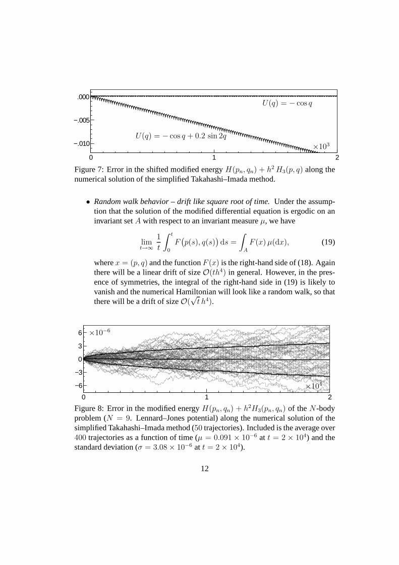
2 is globally defined on the circleS1.This is the situation for the pendulum, whereU(q) = − cos q. We expectthat also higher order terms can be treated in this way, so that no energy driftcan be observed in this situation (see Figure 7, whereh = 0.2, and initialvaluesq(0) = 0, p(0) = 2.5 are used).

• Linear energy drift. In general, without any particular assumption on thepotential, the numerical energy will have a drift of sizeO(th4). E.g., for anon-symmetrically perturbed pendulum withU(q) = − cos q+0.2 sin(2q),for which

∫ 2π

0Uqqq(q)Uq(q)

2dq ≈ 3.77 (see Figure 7).

5E. Hairer, R.I. McLachlan, and R.D. Skeel.On energy conservation of the simplifiedTakahashi–Imada method.ESAIM: M2AN 43:631644, 2009.

11

0 1 2

−.010

−.005

.000

×103

U(q) = − cos q

U(q) = − cos q + 0.2 sin 2q

Figure 7: Error in the shifted modified energyH(pn, qn) + h2H3(p, q) along thenumerical solution of the simplified Takahashi–Imada method.

• Random walk behavior – drift like square root of time.Under the assump-tion that the solution of the modified differential equationis ergodic on aninvariant setA with respect to an invariant measureµ, we have

limt→∞

1

t

∫ t

0

F(p(s), q(s)

)ds =

∫

A

F (x)µ(dx), (19)

wherex = (p, q) and the functionF (x) is the right-hand side of (18). Againthere will be a linear drift of sizeO(th4) in general. However, in the pres-ence of symmetries, the integral of the right-hand side in (19) is likely tovanish and the numerical Hamiltonian will look like a randomwalk, so thatthere will be a drift of sizeO(

√t h4).

0 1 2

−6

−3

0

3

6 ×10−6

×104

Figure 8: Error in the modified energyH(pn, qn) + h2H3(pn, qn) of theN-bodyproblem (N = 9. Lennard–Jones potential) along the numerical solution ofthesimplified Takahashi–Imada method (50 trajectories). Included is the average over400 trajectories as a function of time (µ = 0.091 × 10−6 at t = 2 × 104) and thestandard deviation (σ = 3.08 × 10−6 at t = 2 × 104).

12

5 Existence of global modified Hamiltonian

The theory of generating functions shows that every symplectic one-step methodΦh : (p, q) 7→ (P,Q) can be locally expressed in terms of a functionS(P, q, h) as

p = P + ∇qS(P, q, h), Q = q + ∇pS(P, q, h). (20)

This property allows us to prove the existence of a globally defined modifiedHamiltonian, whenever the generating function is globallydefined.

Theorem 4 Assume that the symplectic methodΦh has a generating function

S(P, q, h) = hS1(P, q) + h2S2(P, q) + h3S3(P, q) + . . . (21)

with smoothSj(P, q) defined on an open setU . Then, the modified differentialequation is a Hamiltonian system with

H(p, q) = H(p, q) + hH2(p, q) + h2H3(p, q) + . . . , (22)

where the functionsHj(p, q) are defined and smooth on the whole ofU .

Proof. The exact solution(P,Q) =(p(t), q(t)

)of the Hamiltonian system corre-

sponding toH(p, q) is given by

p = P + ∇qS(P, q, t), Q = q + ∇P S(P, q, t),

whereS is the solution of the Hamilton–Jacobi differential equation

∂tS(P, q, t) = H(P, q + ∇P S(P, q, t)

), S(P, q, 0) = 0. (23)

SinceH depends on the parameterh, this is also the case forS. Our aim is todetermine the functionsHj(p, q) such that the solutionS(P, q, t) of (23) coincidesfor t = h with (21).

We first expressS(P, q, t) as a series

S(P, q, t) = t S1(P, q, h) + t2S2(P, q, h) + t3S3(P, q, h) + . . . ,

insert it into (23) and compare powers oft. This allows us to obtain the functionsSj(p, q, h) recursively in terms of derivatives ofH:

S1(p, q, h) = H(p, q)

2 S2(p, q, h) =(∂H∂q

· ∂S1

∂P

)(p, q, h) (24)

3 S3(p, q, h) =(∂H∂q

· ∂S2

∂P

)(p, q, h) +

1

2

(∂2H

∂q2

(∂S1

∂P,∂S1

∂P

))(p, q, h).

13

We then writeSj as a series

Sj(p, q, h) = Sj1(p, q) + h Sj2(p, q) + h2Sj3(p, q) + . . . ,

insert it and the expansion (22) forH into (24), and compare powers ofh. Thisyields S1k(p, q) = Hk(p, q) and forj > 1 we see thatSjk(p, q) is a function ofderivatives ofHl with l < k.

The requirementS(p, q, h) = S(p, q, h) finally showsS1(p, q) = S11(p, q),S2(p, q) = S12(p, q) + S21(p, q), etc., so that

Sj(p, q) = Hj(p, q) + “function of derivatives ofHk(p, q) with k < j”.

For a given generating functionS(P, q, h), this recurrence relation allows us todetermine successively theHj(p, q). We see from these explicit formulas that thefunctionsHj are defined on the same domain as theSj.

Example 7 (Symplectic Euler Method) The symplectic Euler method is noth-ing other than (20) withS(P, q, h) = hH(P, q) . Following the constructiveproof of Theorem 4 we obtain

H = H − h

2HpHq +

h2

12

(HppH

2q +HqqH

2p + 4HpqHqHp

)+ . . . . (25)

as the modified Hamiltonian of the symplectic Euler method.

Theorem 5 A symplectic Runge–Kutta method (i.e.,biaij + bjaji = bibj for alli, j) applied to a system with smooth HamiltonianH : U → R (withU ⊂ R

2d anarbitrary open set) has a modified Hamiltonian (22) with smooth functionsHj(y),defined globally onU .

Proof. Let (Pi, Qi) be the internal stages of an implicit Runge–Kutta method(p, q) 7→ (P,Q). It follows from implicit differentiation of the Runge–Kutta equa-tions that, under the conditionbiaij + bjaji = bibj for all i, j, the Runge–Kuttaformulas can be written as (20) with (an idea of Lasagni 1988)

S(P, q, h) = h

s∑

i=1

biH(Pi, Qi) − h2

s∑

i,j=1

biaijHq(Pi, Qi)THp(Pj , Qj).

This shows that the coefficient functionsSj(P, q) can be expressed in terms ofderivatives ofH(P, q).

This theorem extends to partitioned Runge–Kutta methods including the Stormer–Verlet integrators. Theorem 4 implies that all methods based on generating func-tions (e.g., variational integrators) have a globally defined modified Hamiltonian.

14

6 Completely integrable Hamiltonian systems

There is an interesting class of Hamiltonian problems, for which symplectic inte-grators have an improved long-time behavior of the global error. Here and in thefollowing, we denote the standardd-dimensional torus by

Td = R

d/2πZd = {(θ1 mod2π, . . . , θd mod2π) ; θi ∈ R}.

Definition 1 We call a Hamiltonian systemcompletely integrable, if, for every(p0, q0) in the domain ofH(p, q), there exists a symplectic diffeomorphism

(p, q) = ψ(a, θ), 2π-periodic inθ

betweenV × Td andU ⊂ R

2d (whereU is a neighborhood of(p0, q0), andV isopen), such that the Hamiltonian in the new variables becomes

H(p, q) = H(ψ(a, θ)) = K(a).

The variables(a, θ) = (a1, . . . , ad, θ1 mod2π, . . . , θd mod2π) are calledaction-angle variables. In these variables, the system becomes

ai = 0, θi = ωi(a), i = 1, . . . , d

with ωi(a) = ∂∂ai

K(a), and can be solved directlyai(t) = ai0, θi(t) = θi0 +ωi(a0) t, so that we get periodic (or quasi-periodic) flow

(p(t), q(t)

)= ψ

(a0, θ0 + ω(a0) t

).

The following theorem gives a practical characterization of integrability6.

Theorem 6 (Arnold-Liouville) Suppose that for the HamiltonianH(p, q) thereexist smooth functionsF1 = H,F2, . . . , Fd : U → R, U ⊂ R

2d satisfying

(I1) F1, . . . , Fd are in involution, i.e.,{Fi, Fj} = 0, where the Poisson bracketis given by{F,G} = ∇qF

T∇pG−∇pFT∇qG,

(I2) the gradients ofF1, . . . , Fd are everywhere linearly independent,

(I3) the solution trajectories of the Hamiltonian systems with HamiltonianFi

(for i = 1, . . . , d) exist for all times and remain inU .

If, in addition, the level sets{(p, q) ∈ U ; Fi(p, q) = ci, i = 1, . . . , d} are com-pact, then the Hamiltonian system is completely integrable.

6V.I. Arnold, Mathematical Methods of Classical Mechanics, Springer-Verlag, New York,1978, second edition 1989.

15

Example 8 (Motion in central field) Consider the Hamiltonian

H =1

2(p2

1 + p22) + V (r), r =

√q21 + q2

2 ,

with a potentialV (r) that is defined and smooth forr > 0. The Kepler prob-lem corresponds toV (r) = −1/r, and the perturbed Kepler problem toV (r) =−1/r − µ/(3r3). Changing to polar coordinates (see Exercises 3 and 4)

(q1q2

)=

(r cosϕr sinϕ

),

(pr

pϕ

)=

(cosϕ sinϕ

−r sinϕ r cosϕ

) (p1

p2

), (26)

this becomes

H(pr, pϕ, r, ϕ) =1

2

(p2

r +p2

ϕ

r2

)+ V (r).

The system has the angular momentumL = pϕ as a first integral, sinceH doesnot depend onϕ. Clearly,{H,L} = 0 everywhere. The gradients ofH andLare linearly independent unless bothpr = 0 and p2

ϕ = r3V ′(r). By insertingp2

ϕ = 2r2(H − V (r)) and eliminatingr this becomes a condition of the formα(H,L) = 0, which for the Kepler problem readsL2(1 + 2HL2) = 0. Theconditions of Theorem 6 are thus satisfied on the domain

U = {(pr, pϕ, r, ϕ) ; r > 0, α(H,L) 6= 0}.Example 9 (Toda lattice) This is a system of particles on a line interacting pair-wise with exponential forces. The motion is determined by the Hamiltonian

H(p, q) =

n∑

k=1

(1

2p2

k + exp(qk − qk+1))

with periodic boundary conditions:qn+1 = q1. With the notationak = −12pk,

bk = 12exp

(12(qk − qk+1)

), all n eigenvalues of the matrix

L =

a1 b1 bnb1 a2 b2 0

b2. . . . . .

0. . . an−1 bn−1

bn bn−1 an

are first integrals of the system. It can be shown (here without proof) that thissystem is completely integrable

Many important problems in celestial mechanics are small perturbations ofintegrable systems, e.g., planetary motion.

16

7 Linear error growth for integrable systems

We consider a completely integrable Hamiltonian system

p = −∇qH(p, q), q = ∇pH(p, q). (27)

with real analytic Hamiltonian. We let(p, q) = ψ(a, θ) be the symplectic dif-feomorphism that transforms (27) to action-angle variables, and we denote theinverse transformation by(a, θ) =

(I(p, q),Θ(p, q)

). Consequently, the compo-

nentsI1, . . . , Id of I are first integrals of the system, i.e.,I(p(t), q(t)) = I(p0, q0)for all t. In the action-angle variables, the Hamiltonian isK(a) = H(p, q), andwe denote the vector of frequencies byω(a) = ∇K(a). We consider this in aneighbourhood of somea∗ ∈ R

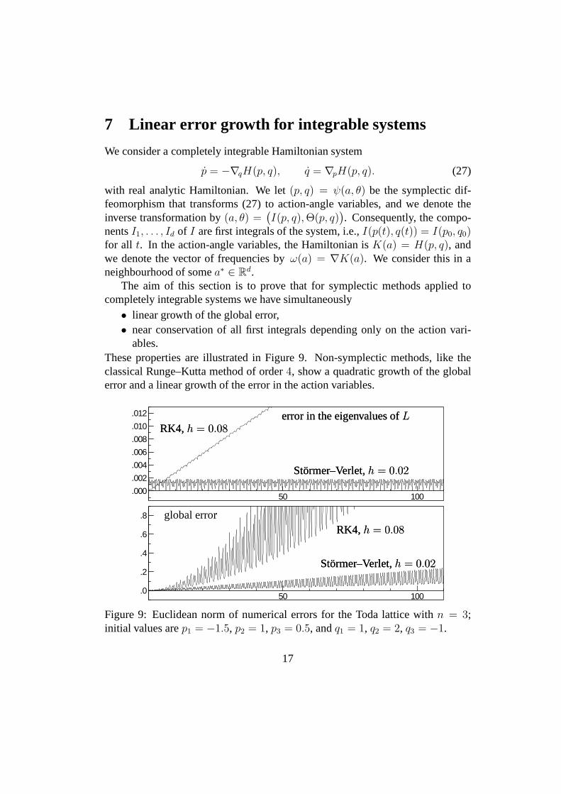
d.The aim of this section is to prove that for symplectic methods applied to

completely integrable systems we have simultaneously• linear growth of the global error,• near conservation of all first integrals depending only on the action vari-

ables.These properties are illustrated in Figure 9. Non-symplectic methods, like theclassical Runge–Kutta method of order4, show a quadratic growth of the globalerror and a linear growth of the error in the action variables.

50 100.000.002.004.006.008.010.012

50 100.0

.2

.4

.6

.8

error in the eigenvalues ofL

Stormer–Verlet,h = 0.02

RK4,h = 0.08error in the eigenvalues ofL

Stormer–Verlet,h = 0.02

RK4,h = 0.08

global error

Stormer–Verlet,h = 0.02

RK4,h = 0.08

global error

Stormer–Verlet,h = 0.02

RK4,h = 0.08

Figure 9: Euclidean norm of numerical errors for the Toda lattice with n = 3;initial values arep1 = −1.5, p2 = 1, p3 = 0.5, andq1 = 1, q2 = 2, q3 = −1.

17

Theorem 7 Consider• completely integrable Hamiltonian system with real-analytic Hamiltonian• symplectic integrator of orderr with globally defined modified Hamiltonian• strong non-resonance condition forω(a∗)

|k · ω(a∗)| ≥ γ|k|−ν , k ∈ Zd, k 6= 0 (28)

• ‖I(p0, q0) − a∗‖ ≤ Const | log h|−ν−1

Then, there exist constantsC, h0 such that forh ≤ h0 and fort = nh ≤ h−r thenumerical solution satisfies

‖(pn, qn) − (p(t), q(t))‖ ≤ C t hr

‖I(pn, qn) − I(p0, q0)‖ ≤ C hr.

Proof. Let us mention (without proof) that forν > d − 1 the set of frequenciesin a fixed ball that do not satisfy (28) has Lebesgue measure bounded bycγ.Therefore, almost all frequencies satisfy (28) for someγ > 0.

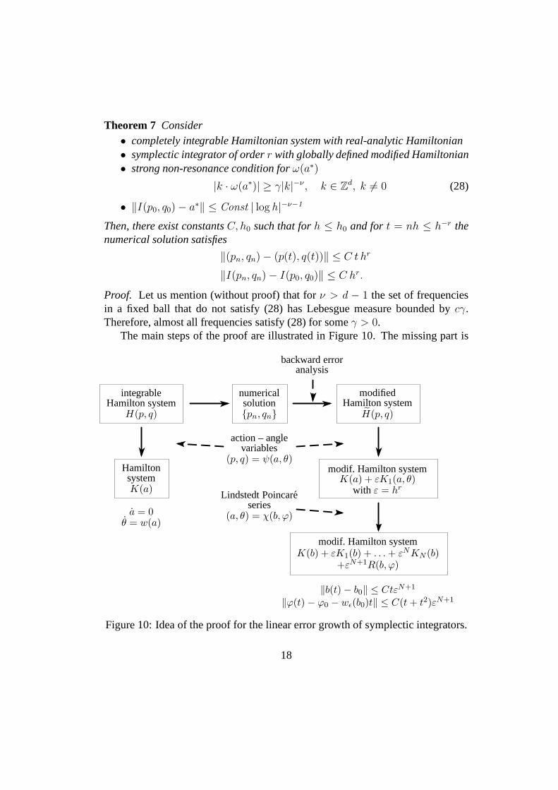
The main steps of the proof are illustrated in Figure 10. The missing part is

backward erroranalysis

integrableHamilton system

H(p, q)

numericalsolution{pn, qn}

modifiedHamilton system

H(p, q)

HamiltonsystemK(a)

action – anglevariables

(p, q) = ψ(a, θ)modif. Hamilton systemK(a) + εK1(a, θ)

with ε = hr

a = 0θ = w(a)

Lindstedt Poincareseries

(a, θ) = χ(b, ϕ)

modif. Hamilton systemK(b) + εK1(b) + . . .+ εNKN (b)

+εN+1R(b, ϕ)

‖b(t) − b0‖ ≤ CtεN+1

‖ϕ(t) − ϕ0 − wǫ(b0)t‖ ≤ C(t+ t2)εN+1

Figure 10: Idea of the proof for the linear error growth of symplectic integrators.

18

the recursive elimination of the angle-variables by the useof a Lindstedt–Poincareseries. This will be discussed in the following (omitting technical details).

We consider a perturbed Hamiltonian

K(a, θ) = K(a) + εK1(a, θ).

The problem is to find a symplectic transformation(a, θ) = χ(b, ϕ) which elimi-nates the angle variableθ as far as possible. We look for a transformation of theform

b = a−∇θS(b, θ), ϕ = θ + ∇bS(b, θ),

where the generating function is given by a truncated series

S(b, θ) = εS1(b, θ) + ε2S2(b, θ) + . . .+ εNSN(b, θ)

with coefficient functions that are2π-periodic inθ. Such a transformation isO(ε)close to the identity. In the new variables the Hamiltonian is

K(χ(b, ϕ)) = K(a, θ) = K(b+ ∇θS(b, θ), θ)

= K(b) + ε(ω(b) · ∇θS1(b, θ) +K1(b, θ)

)+ O(ε2)

whereω(b) = ∇K(b). We aim in findingS1 such that

ω(b) · ∇θS1(b, θ) +K1(b, θ)

does not depend onθ. Expanding the periodic functions into Fourier series

S1(b, θ) =∑

k∈Zd

sk(b)ei k·θ, K1(b, θ) =

∑

k∈Zd

hk(b)ei k·θ,

we obtain a formal solution from

sk(b) = − hk(b)

i k · ω(b), k 6= 0.

At this point we are struck by theproblem of small denominators. For any valuesof the frequenciesωj(b), the denominatork · ω(b) = k1ω1(b) + · · · + kdωd(b)becomes arbitrarily small for somek = (k1, . . . , kd) ∈ Z

d, and even vanishesif the frequencies are rationally dependent. Using the non-resonace condition(28) and the fast decay of Fourier coefficients for analytic functions permits toovercome this difficulty.

Further coefficients of the generating functionS(b, θ) can be constructed in asimilar way.

19

8 Exercises

1. Change the Maple script of Example 1 in such a way that the modifiedequations for the implicit Euler method, the implicit midpoint rule, or thetrapezoidal rule are obtained. Observe that for symmetric methods one getsexpansions in even powers ofh.

2. Compute a first integral of the Lotka–Volterra equations (Example 2) and ofthe truncated modified equation for the symplectic Euler method.

3. LetQ = χ(q) be a change of position coordinates. Prove that the relationp = χ′(q)TP extend this to a symplectic mapping(p, q) 7→ (P,Q).Hint. Consider the generating functionS(P, q) = PTχ(q).

4. Let y = ψ(z) be a symplectic change of coordinates. Prove that it trans-formsy = J−1∇H(y) into z = J−1∇K(z) withK(z) = H(y) = H

(ψ(z)

).

5. (Field & Nijhoff 2003)7 Apply the symplectic Euler method to the systemwith HamiltonianH(p, q) = ln(α+ p) + ln(β + q). Compute the modifiedHamiltonian and prove that the series converges for sufficiently small stepsizes.Hint. The method conserves exactlyI(p, q) = (α + p)(β + q). Find lineartwo-term recursions for{pn} and{qn}, and use the ideas of Example 3.Result.

H(p, q) = H(p, q) −∑

k≥1

hk I(p, q)−k

k(k + 1).

6. Consider a differential equationy = f(y) with a divergence-free vectorfield, and apply a volume-preserving integrator. Show that every truncationof the modified equation has again a divergence-free vector field.Hint. Adapt the proof by induction of Theorem 2.

7C.M. Field & F.W. Nijhoff, A note on modified Hamiltonians for numerical integrations ad-mitting an exact invariant, Nonlinearity 16 (2003) 1673–1683.

20