28 R.H. NOCHETTO

3. Lecture 3: Adaptivity II: General Operators and Extensions

In this lecture we discuss new ideas to prove convergence of AFEM for general operator (1.3) insections 3.1-3.4, along with extensions in section 3.5. We use the notation

eh := u− uh, eH := u− uH , εH := uh − uH .

3.1. Quasi-Orthogonality. If b 6= 0 in (1.7), then the bilinear form B is no longer symmetric, andthus a scalar product. Therefore, the orthogonality relation (2.23) between u − uH and uh − uH ,the so-called Pythagoras equality, fails to hold. We have instead a perturbation result referred to asquasi-orthogonality provided that the initial mesh is fine enough.

Lemma 3.1 (Quasi-orthogonality). There exists a constant C∗ > 0, solely depending on the shaperegularity constant γ∗ and a number 0 < s ≤ 1 dictated only by the interior angles of ∂Ω, such that ifthe meshsize h0 of the initial mesh satisfies C∗hs

0 ‖b‖L∞ < 1, then

|||u− uh|||2≤ Λ0 |||u− uH |||

2− |||uh − uH |||

2,(3.1)

where Λ0 := (1− C∗hs0 ‖b‖L∞)−1. The equality holds provided b = 0 in Ω.

Proof. In view of Galerkin orthogonality (1.13), namely B[eh, v] = 0, for all v ∈ Vh, we have

|||eH |||2

= |||eh|||2

+ |||εH |||2+ B[εH , eh].

If b = 0, then B is symmetric and B[εH , eh] = B[eh, εH ] = 0. For b 6= 0, instead, B[εH , eh] 6= 0, andwe must account for this term. It is easy to see that div b = 0 and integration by parts yield

B[εH , eh] = B[eh, εH ] + 〈b · ∇εH , eh〉 − 〈b · ∇eh, εH〉 = 2 〈b · ∇εH , eh〉 .

Hence

|||eh|||2

= |||eH |||2− |||εH |||

2− 2 〈b · ∇εH , eh〉 .

Using Cauchy-Schwarz inequality and replacing the H1(Ω)-norm by the energy norm we have, for anyδ > 0 to be chosen later,

−2 〈b · ∇εH , eh〉 ≤ δ ‖eh‖2L2 +

‖b‖2L∞

δcB|||εH |||

2.

We then realize the need to relate L2(Ω) and energy norms to replace ‖eh‖L2 by |||eh|||. This requiresa standard duality argument whose proof is reported in Ciarlet [15].

Lemma 3.2 (Duality). Let f ∈ L2(Ω) and u ∈ H1+s(Ω) for some 0 < s ≤ 1 be the solution of (1.6),where s depends on the interior angles of ∂Ω (s = 1 if Ω is convex). Then, there exists a constant CD,depending only on the shape regularity constant γ∗ and the data of (1.3) such that

‖eh‖L2 ≤ CDhs ‖eh‖V .(3.2)

Inserting this estimate in the preceding two bounds, and using h ≤ h0, the meshsize of the initial

mesh, in conjunction with cB‖eh‖2V≤ |||eh|||

2we deduce

(1− δCD

2c−1B h2s

0

)|||eh|||

2≤ |||eH |||

2−

(1− ‖b‖

2L∞(δcB)−1

)|||εH |||

2.

We now choose δ =‖b‖

L∞

CDhs

0

to equate both parenthesis, as well as h0 sufficiently small for δCD2h2s

0 c−1B =

C∗hs0 ‖b‖L∞ < 1 with C∗ := CD/cB. We end up with

|||eh|||2≤

1

1− C∗hs0 ‖b‖L∞

|||eH |||2− |||εH |||

2.

This implies (3.1) and concludes the proof.

ADAPTIVE FINITE ELEMENT METHODS FOR ELLIPTIC PDE 29

3.2. Error and Oscillation Reduction. In order to extend the theory of section 2.4 to the operatorL of (1.3), we first notice that the local lower bound of Lemma 2.9 is still valid in this context. Thisis because its proof does not depend on the specific structure of the oscillation oscH . However, oscH

cannot be related directly to osch as in Lemma 2.10, because oscH and osch depend on uH and uh

respectively. The next lemma accounts for this dependence.

Lemma 3.3 (Oscillation Reduction). There exist constants 0 < ρ1 < 1 and 0 < ρ2, only depending onγ∗ and θ0, such that

osch(Ω)2≤ ρ1oscH(Ω)

2+ ρ2 |||uh − uH |||

2.(3.3)

Proof. The proof hinges on the Marking Strategy O and the Interior Node Property. We recall that if

T ∈ Th is contained in T ′ ∈ TH , then REFINE gives a reduction factor γ0 < 1 of element size:

hT ≤ γ0HT ′ .(3.4)

The proof proceeds in three steps as follows.1. Relation between Oscillations. We would like to relate osch(T ′) and oscH(T ′) for any T ′ ∈ TH .

To this end, we note that for all T ∈ Th contained in T ′, we can write

RT (uh) = RT (uH)−LT (εH) in T,

where εH = uh − uH as before and

LT (εH) := − div (A∇εH) + b · ∇εH + c εH in T.

By Young’s inequality, we have for all δ > 0

osch(T )2 = h2T

∥∥∥RT (uh)−RT (uh)∥∥∥

2

L2(T )

≤ (1+δ)h2T

∥∥∥RT (uH)−RT (uH)∥∥∥

2

L2(T )+(1+δ−1)h2

T

∥∥∥LT (εH)−LT (εH)∥∥∥

2

L2(T ),

where RT (uh), RT (uH), and LT (εH) are L2-projections of RT (uh), RT (uH), and LT (εH) onto poly-nomials of degree ≤ n− 1 on T . We next observe that∥∥∥LT (εH)− LT (εH)

∥∥∥L2(T )

≤ ‖LT (εH)‖L2(T )

and that, according to (3.4),

hT ≤ γT ′HT ′

provided γT ′ = γ0 if T ′ ∈ TH and γT ′ = 1 otherwise. Therefore, if Th(T ′) denotes all T ∈ Th containedin T ′,

(3.5)

osch(T ′)2

=∑

T∈Th(T ′)

osch(T )2

≤ (1 + δ)γ2T ′oscH(T ′)

2+ (1 + δ−1)

∑

T∈Th(T ′)

h2T ‖LT (εH)‖

2L2(T ),

since RT (uH) = RT ′(uH) and RT (uH) is the best L2-approximation of RT ′(uH) in T .2. Estimate of LT (εH). In order to estimate ‖LT (εH)‖L2(T ) in terms of ‖εH‖H1(T ), we first split it

as follows

‖LT (εH)‖L2(T ) ≤ ‖div(A∇εH)‖L2(T ) + ‖b · ∇εH‖L2(T ) + ‖c εH‖L2(T )

and denote these terms NA, NB , and NC , respectively. Since

NA ≤ ‖(div A) · ∇εH‖L2(T ) + ‖A : H(εH)‖L2(T )

where H(εH) is the Hessian of εH in T , invoking the Lipschitz continuity of A together with an inverseestimate in T , we infer that

NA ≤ CA

(‖∇εH‖L2(T ) + h−1

T ‖∇εH‖L2(T )

),

30 R.H. NOCHETTO

where CA depends on A and the shape regularity constant γ∗. Besides, we readily have

NB ≤ CB ‖∇εH‖L2(T ) , NC ≤ CC ‖εH‖L2(T ) ,

where CB , CC depend on b, c. Combining these estimates, we arrive at

h2T ‖LT (εH)‖2L2(T ) ≤ C∗ ‖εH‖

2H1(T ) .(3.6)

3. Choice of δ. We insert (3.6) into (3.5) and add over T ′ ∈ TH . Recalling the definition of γT ′ andutilizing (2.18), we deduce

∑

T ′∈TH

γ2T ′oscH(T ′)

2= γ2

0

∑

T ′∈bTH

oscH(T ′)2

+∑

T ′∈TH\bTH

oscH(T ′)2

= oscH(Ω)2− (1− γ2

0)∑

T ′∈bTH

oscH(T ′)2

≤ (1− (1− γ20)θ2))oscH(Ω)

2,

where theta0 is the user’s parameter in (2.18). Moreover, since C∗ ‖εH‖2H1 ≤ Co |||εH |||

2with Co =

C∗c−1B in light of the equivalence between energy and H1 norms, we end up with

osch(Ω)2≤ (1 + δ)(1− (1− γ2

0)θ2)oscH(Ω)2

+ (1 + δ−1)Co |||εH |||2.

We finally choose δ sufficiently small so that

ρ1 = (1 + δ)(1− (1− γ20)θ2) < 1, ρ2 = (1 + δ−1)Co.

to complete the proof.

3.3. Convergence for General Operators. Since error and oscillation are now coupled, in orderto prove convergence we need to handle them together. This leads to a novel argument and result, thecontraction property (3.7) below, according to which both error and oscillation decrease together.

Theorem 3.4 (Convergence of AFEM). Let ukk∈N0be a sequence of finite element solutions cor-

responding to a sequence of nested finite element spacesV

k

k∈N0

produced by AFEM. There exist

constants σ, γ > 0, and 0 < ξ < 1, depending solely on the mesh regularity constant γ∗, data, param-eters θE and θ0, and a number 0 < s ≤ 1 dictated by interior angles of ∂Ω, such that if the initialmeshsize h0 satisfies hs

0‖b‖L∞c−1B < σ, then for any two consecutive iterates k and k + 1, we have

|||u− uk+1|||2

+ γ osck+1(Ω)2≤ ξ2

(|||u− uk|||

2+ γ osck(Ω)

2)

.(3.7)

Therefore AFEM converges with a linear rate ξ, namely,

|||u− uk|||2

+ γ osck(Ω)2≤ C0 ξ2k,

where C0 := |||u− u0|||2

+ γ osc0(Ω)2.

Proof. We just prove the contraction property (3.7), which obviously implies the decay estimate. Forconvenience, we introduce the notation

ek := |||u− uk||| , εk := |||uk+1 − uk||| , osck := osck(Ω) .

The idea is to use the quasi-orthogonality (3.1) and replace the term |||uk+1 − uk|||2

using new resultsof error and oscillation reduction estimates (2.21) and (3.3). We proceed in three steps as follows.

1. We first get a lower bound for εk in terms of ek. To this end, we use Marking Strategy E andthe upper bound (2.5) to write

θ2Ee2

k ≤ C1θ2Eηk(Ω)2 ≤ C1

∑

T∈cTk

ηk(T )2.

ADAPTIVE FINITE ELEMENT METHODS FOR ELLIPTIC PDE 31

Adding (2.21) of Lemma 2.9 over all marked elements T ∈ Tk, and observing that each element can

be counted at most D := d + 2 times due to overlap of the sets ωT , together with ‖v‖2V≤ c−1

B |||v|||2 for

all v ∈ H10 (Ω), we arrive at

θ2Ee2

k ≤DC1

C2cBε2

k +DC1

C2osc2

k.

If Λ1 := cBC2

DC1

θ2E , Λ2 := cB , then this implies the lower bound for ε2

k,

ε2k ≥ Λ1e

2k − Λ2osc2

k.(3.8)

2. If h0 is sufficiently small so that the quasi-orthogonality (3.1) of Lemma 3.1 holds with Λ0 =(1− C∗hs

0 ‖b‖L∞ c−1B )−1, then

e2k+1 ≤ Λ0e

2k − ε2

k.

Replacing the fraction βε2k of ε2

k via (3.8) we obtain

e2k+1 ≤ (Λ0 − βΛ1)e

2k + βΛ2osc2

k − (1− β)ε2k,

where 0 < β < 1 is a constant to be chosen suitably. We now assert that it is possible to chose h0

compatible with Lemma 3.1 and also that

0 < α := Λ0 − βΛ1 < 1.

A simple calculation shows that this is the case provided

hs0 ‖b‖L∞ c−1

B <βΛ1

C∗(1 + βΛ1)<

1

C∗,

i.e., hs0 ‖b‖L∞ c−1

B < σ with σ := βΛ1

C∗(1+βΛ1) . Consequently

e2k+1 ≤ αe2

k + βΛ2osc2k − (1− β)ε2

k.(3.9)

3. To remove the last term of (3.9) we resort to the oscillation reduction estimate of Lemma 3.3

osc2k+1 ≤ ρ1osc2

k + ρ2ε2k.

We multiply it by (1− β)/ρ2 and add it to (3.9) to deduce

e2k+1 +

1− β

ρ2osc2

k+1 ≤ α e2k +

(βΛ2 +

ρ1

ρ2(1− β)

)osc2

k.

If γ := 1−βρ2

, then we would like to choose β < 1 in such a way that

βΛ2 + ρ1γ = µγ

for some µ < 1. A simple calculation yields

β =

µ−ρ1

ρ2

Λ2 + µ−ρ1

ρ2

,

and shows that ρ1 < µ < 1 guarantees that 0 < β < 1. Therefore,

e2k+1 + γ osc2

k+1 ≤ α e2k + µγ osc2

k,

and the asserted estimate (3.7) follows upon taking ξ = max(α, µ) < 1.

Remark 3.5 (Comparison with Theorem 2.13). In Thereom 2.13, and [34, 35], the oscillation is inde-pendent of discrete solutions, i.e. ρ2 = 0, and is reduced by the factor ρ1 < 1 in (3.3). Consequently,Step 3 above is avoided by setting β = 1 and the decay of ek and osck is monitored separately. Sincethis is no longer possible, ek and osck are now combined and decreased together.

Remark 3.6 (Splitting of εk). The idea of splitting εk is already used by Chen and Jia [13] in examiningone time step for the heat equation. This is because a mass (zero order) term naturally occurs, whichdid not take place in [34, 35]. The elliptic operator is just the Laplacian in [13].

32 R.H. NOCHETTO

Remark 3.7 (Effect of Convection). Assuming that hs0 ‖b‖L∞ c−1

B < σ implies that the local Pecletnumber is sufficiently small for the Galerkin method not to exhibit oscillations. This appears tobe essential for u0 to contain relevant information and guide correctly the adaptive process. Thisrestriction is difficult to verify in practice because it involves unknown constants.However, startingfrom coarser meshes than needed in theory does not seem to be a problem in practice (see simulationsin §3.4.2).

Remark 3.8 (Vanishing Convection). If b = 0, then Theorem 3.4 has no restriction on the initialmesh. This thus extends the convergent result of Morin et al. [34, 35] to variable diffusion coefficientand zero order terms.

Remark 3.9 (Optimal β). The choice of β can be optimized. In fact, we can easily see that

α = Λ0 − βΛ1, µ = ρ1 +β

1− βρ2Λ2

yields a unique value 0 < β∗ < 1 for which α = µ and the contraction constant ξ of Theorem 3.4 isminimal. This β∗ depends on geometric constant Λ0, Λ1, Λ2 as well on θE , θ0 and h0, but it is notcomputable.

3.4. Numerical Experiments. For convenience of presentation, we introduce the following notation:• DOF := number of elements in a given mesh, which is comparable with number of degree of freedoms;

• EOC := log(e(k−1)/e(k))log(DOF(k)/DOF(k−1)) , experimental order of convergence, e(k) :=‖u− uk‖H1 ;

• EOC(η) :=log(ηk−1/ηk)

log(DOF(k)/DOF(k−1)) , experimental order of convergence of estimator, ηk := ηk(Ω);

• Ze := e(k)/e(k − 1) and Zo := osck/osck−1, reduction factors of error and oscillation;• Eff := ek/ηk, effectivity index, i.e. the ratio between the error and the estimator. This ratio does infact give an estimate to constant C1 for upper bound (2.5).• ME and MO are the number of marked elements due to Marking Strategy E and the additionalmarked elements due to Marking Strategy O, respectively.

The experimental order of convergence (EOC) measures how the error (or estimator) decreases as

the number of DOF increases. In fact we have errork ≈ C DOFk−EOC.

3.4.1. Example: Oscillatory Coefficients and Nonconvex Domain. We consider the PDE (1.3) withDirichlet boundary condition u = g on the nonconvex L-shape domain Ω := (−1, 1)2\ [0, 1]× [−1, 0].We also take the exact solution

u(r) = r2

3 sin(2

3θ),

where r2 := x2+y2 and θ := tan−1(y/x) ∈ [0, 2π). We deal with variable coefficients A(x, y) = a(x, y)I,b(x, y) = 0 and c(x, y) defined by

a(x, y) =1

4 + P (sin( 2πxε ) + sin( 2πy

ε )),(3.10)

c(x, y) = Ac(cos2(lx) + cos2(lx)) ,(3.11)

where P, ε, Ac, and l are parameters. The functions f in (1.3) and g are defined accordingly. Theresults are shown in Tables 3.1 and 3.2 and Figure 3.1. The observations and conclusions of thisexperiment are as follows:• AFEM gives an optimal rate of convergence of order ≈ 0.5, while standard uniform refinementachieves the suboptimal rate of 0.3 as expected from theory.• Both AFEM and FEM with uniform refinement perform with effectivity index Eff ≈ 2.0, which givethe estimate of constant C1 ≈ 0.5 for upper bound (2.5); no weights have been used in (2.4). For AFEM,the reduction factors of error and oscillation are approximately 0.7 and 0.5 as DOF increases (Table3.1). The oscillation thus decreases faster than the error and becomes insignificant asymptotically fork large. In addition, AFEM outperforms FEM in terms of CPU time vs energy error.• Figure 3.1 depicts the effect of a corner singularity and rapid variation of diffusion coefficient a(x, y)in mesh grading; c does not play much role.

ADAPTIVE FINITE ELEMENT METHODS FOR ELLIPTIC PDE 33

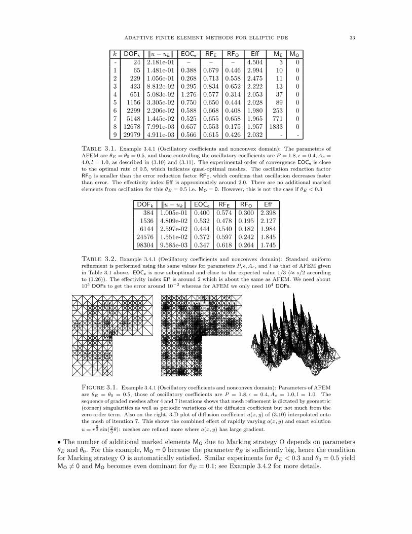
k DOFk |||u− uk||| EOCe RFE RFO Eff ME MO

- 24 2.181e-01 – – – 4.504 3 01 65 1.481e-01 0.388 0.679 0.446 2.994 10 02 229 1.056e-01 0.268 0.713 0.558 2.475 11 03 423 8.812e-02 0.295 0.834 0.652 2.222 13 04 651 5.083e-02 1.276 0.577 0.314 2.053 37 05 1156 3.305e-02 0.750 0.650 0.444 2.028 89 06 2299 2.206e-02 0.588 0.668 0.408 1.980 253 07 5148 1.445e-02 0.525 0.655 0.658 1.965 771 08 12678 7.991e-03 0.657 0.553 0.175 1.957 1833 09 29979 4.911e-03 0.566 0.615 0.426 2.032 - -

Table 3.1. Example 3.4.1 (Oscillatory coefficients and nonconvex domain): The parameters ofAFEM are θE = θ0 = 0.5, and those controlling the oscillatory coefficients are P = 1.8, ε = 0.4, Ac =4.0, l = 1.0, as described in (3.10) and (3.11). The experimental order of convergence EOCe is closeto the optimal rate of 0.5, which indicates quasi-optimal meshes. The oscillation reduction factorRFO is smaller than the error reduction factor RFE, which confirms that oscillation decreases fasterthan error. The effectivity index Eff is approximately around 2.0. There are no additional markedelements from oscillation for this θE = 0.5 i.e. MO = 0. However, this is not the case if θE < 0.3

DOFk |||u− uk||| EOCe RFE RFO Eff

384 1.005e-01 0.400 0.574 0.300 2.3981536 4.809e-02 0.532 0.478 0.195 2.1276144 2.597e-02 0.444 0.540 0.182 1.984

24576 1.551e-02 0.372 0.597 0.242 1.84598304 9.585e-03 0.347 0.618 0.264 1.745

Table 3.2. Example 3.4.1 (Oscillatory coefficients and nonconvex domain): Standard uniformrefinement is performed using the same values for parameters P, ε,Ac, and l as that of AFEM givenin Table 3.1 above. EOCe is now suboptimal and close to the expected value 1/3 (≈ s/2 accordingto (1.26)). The effectivity index Eff is around 2 which is about the same as AFEM. We need about105 DOFs to get the error around 10−2 whereas for AFEM we only need 104 DOFs.

Figure 3.1. Example 3.4.1 (Oscillatory coefficients and nonconvex domain): Parameters of AFEMare θE = θ0 = 0.5, those of oscillatory coefficients are P = 1.8, ε = 0.4, Ac = 1.0, l = 1.0. Thesequence of graded meshes after 4 and 7 iterations shows that mesh refinement is dictated by geometric(corner) singularities as well as periodic variations of the diffusion coefficient but not much from thezero order term. Also on the right, 3-D plot of diffusion coefficient a(x, y) of (3.10) interpolated ontothe mesh of iteration 7. This shows the combined effect of rapidly varying a(x, y) and exact solution

u = r2

3 sin( 2

3θ): meshes are refined more where a(x, y) has large gradient.

• The number of additional marked elements MO due to Marking strategy O depends on parametersθE and θ0. For this example, MO = 0 because the parameter θE is sufficiently big, hence the conditionfor Marking strategy O is automatically satisfied. Similar experiments for θE < 0.3 and θ0 = 0.5 yieldMO 6= 0 and MO becomes even dominant for θE = 0.1; see Example 3.4.2 for more details.

34 R.H. NOCHETTO

3.4.2. Example: Convection-Dominated Convection. We consider the convection dominated-diffusionelliptic model problem (1.3) with Dirichlet boundary condition u = g on convex domain Ω := (0, 1)2,with isotropic diffusion coefficient A = εI, ε = 10−3, convection velocity b = (y, 1

2 −x) and c = f = 0;note that div b = 0. The Dirichlet boundary condition g(x, y) on ∂Ω, a pulse, is the continuouspiecewise linear function given by

g(x, y) =

1 .2 + τ ≤ x ≤ .5− τ ; y = 0 ,

0 ∂Ω \ .2 ≤ x ≤ .5; y = 0 ,

linear (.2 ≤ x ≤ .2 + τ) or (.5− τ ≤ x ≤ .5); y = 0 ,

(3.12)

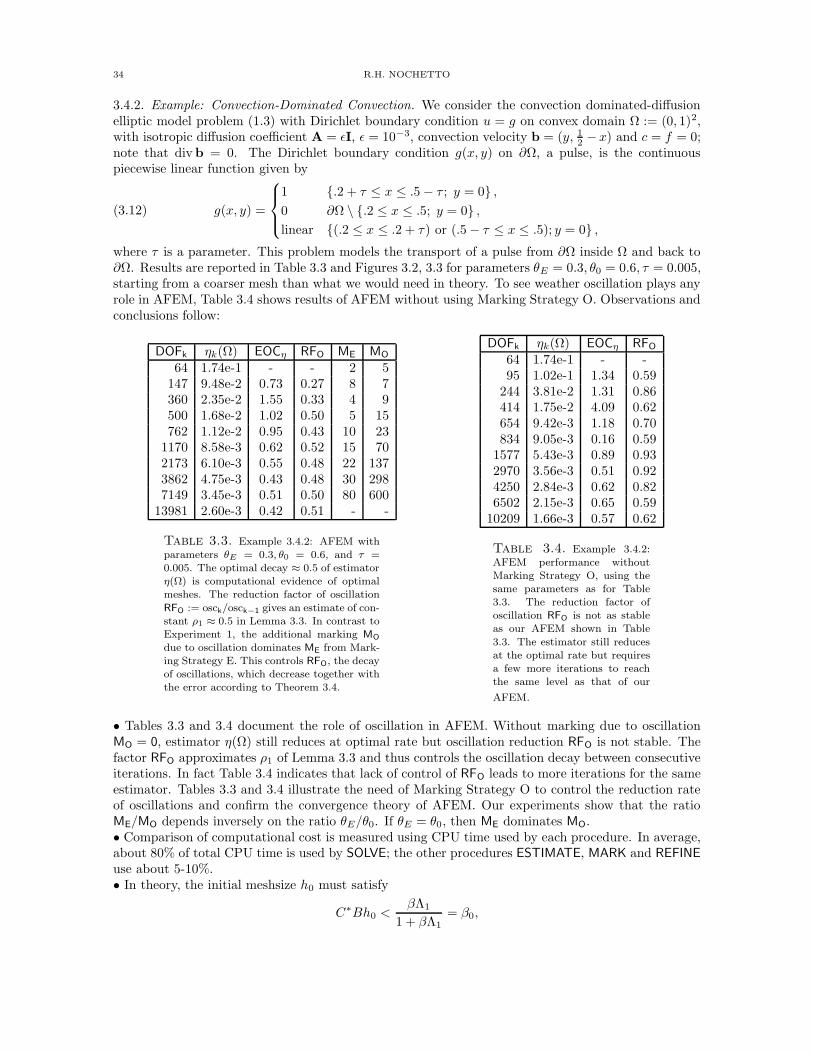
where τ is a parameter. This problem models the transport of a pulse from ∂Ω inside Ω and back to∂Ω. Results are reported in Table 3.3 and Figures 3.2, 3.3 for parameters θE = 0.3, θ0 = 0.6, τ = 0.005,starting from a coarser mesh than what we would need in theory. To see weather oscillation plays anyrole in AFEM, Table 3.4 shows results of AFEM without using Marking Strategy O. Observations andconclusions follow:

DOFk ηk(Ω) EOCη RFO ME MO

64 1.74e-1 - - 2 5147 9.48e-2 0.73 0.27 8 7360 2.35e-2 1.55 0.33 4 9500 1.68e-2 1.02 0.50 5 15762 1.12e-2 0.95 0.43 10 23

1170 8.58e-3 0.62 0.52 15 702173 6.10e-3 0.55 0.48 22 1373862 4.75e-3 0.43 0.48 30 2987149 3.45e-3 0.51 0.50 80 600

13981 2.60e-3 0.42 0.51 - -

Table 3.3. Example 3.4.2: AFEM withparameters θE = 0.3, θ0 = 0.6, and τ =0.005. The optimal decay ≈ 0.5 of estimatorη(Ω) is computational evidence of optimalmeshes. The reduction factor of oscillation

RFO := osck/osck−1 gives an estimate of con-stant ρ1 ≈ 0.5 in Lemma 3.3. In contrast toExperiment 1, the additional marking MO

due to oscillation dominates ME from Mark-ing Strategy E. This controls RFO, the decayof oscillations, which decrease together withthe error according to Theorem 3.4.

DOFk ηk(Ω) EOCη RFO

64 1.74e-1 - -95 1.02e-1 1.34 0.59

244 3.81e-2 1.31 0.86414 1.75e-2 4.09 0.62654 9.42e-3 1.18 0.70834 9.05e-3 0.16 0.59

1577 5.43e-3 0.89 0.932970 3.56e-3 0.51 0.924250 2.84e-3 0.62 0.826502 2.15e-3 0.65 0.59

10209 1.66e-3 0.57 0.62

Table 3.4. Example 3.4.2:AFEM performance withoutMarking Strategy O, using thesame parameters as for Table3.3. The reduction factor ofoscillation RFO is not as stableas our AFEM shown in Table

3.3. The estimator still reducesat the optimal rate but requiresa few more iterations to reachthe same level as that of our

AFEM.

• Tables 3.3 and 3.4 document the role of oscillation in AFEM. Without marking due to oscillationMO = 0, estimator η(Ω) still reduces at optimal rate but oscillation reduction RFO is not stable. Thefactor RFO approximates ρ1 of Lemma 3.3 and thus controls the oscillation decay between consecutiveiterations. In fact Table 3.4 indicates that lack of control of RFO leads to more iterations for the sameestimator. Tables 3.3 and 3.4 illustrate the need of Marking Strategy O to control the reduction rateof oscillations and confirm the convergence theory of AFEM. Our experiments show that the ratioME/MO depends inversely on the ratio θE/θ0. If θE = θ0, then ME dominates MO.• Comparison of computational cost is measured using CPU time used by each procedure. In average,about 80% of total CPU time is used by SOLVE; the other procedures ESTIMATE, MARK and REFINE

use about 5-10%.• In theory, the initial meshsize h0 must satisfy

C∗Bh0 <βΛ1

1 + βΛ1= β0,

ADAPTIVE FINITE ELEMENT METHODS FOR ELLIPTIC PDE 35

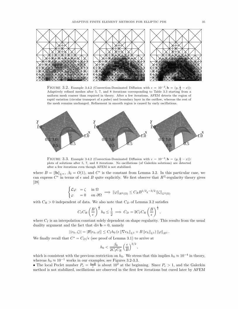
Figure 3.2. Example 3.4.2 (Convection-Dominated Diffusion with ε = 10−3,b = (y, 1

2− x)):

Adaptively refined meshes after 5, 7, and 8 iterations corresponding to Table 3.3 starting from auniform mesh coarser than required in theory. After a few iterations, AFEM detects the region ofrapid variation (circular transport of a pulse) and boundary layer in the outflow, whereas the rest ofthe mesh remains unchanged. Refinement in smooth region is caused by early oscillations.

y1.0

1.0x

0.50.50.5

1.0

y1.0

1.0x

0.50.50.5

1.0

y1.0

1.0x

0.50.50.5

1.0

Figure 3.3. Example 3.4.2 (Convection-Dominated Diffusion with ε = 10−3,b = (y, 1

2− x)):

plots of solutions after 5, 7, and 8 iterations. No oscillations (of Galerkin solutions) are detectedafter a few iterations even though AFEM is not stabilized.

where B = ‖b‖L∞ , β0 = O(1), and C∗ is the constant from Lemma 3.2. In this particular case, wecan express C∗ in terms of ε and B quite explicitly. We first observe that H2-regularity theory gives[28]

Lϕ = ζ in Ω

ϕ = 0 on ∂Ω=⇒ ‖ϕ‖H2(Ω) ≤ CRB1/2ε−3/2 ‖ζ‖L2(Ω)

with CR > 0 independent of data. We also note that CD of Lemma 3.2 satisfies

CICR

(B

ε

) 3

2

h0 ≤1

2=⇒ CD = 2CICR

(B

ε

) 1

2

,

where CI is an interpolation constant solely dependent on shape regularity. This results from the usualduality argument and the fact that div b = 0, namely

|〈eh, ζ〉| = |B[eh, ϕ]| ≤ CIh0 (ε ‖∇eh‖L2 + B ‖eh‖L2) ‖ϕ‖H2 .

We finally recall that C∗ = CD/ε (see proof of Lemma 3.1) to arrive at

h0 <β0

2CICR

( ε

B

)3/2

,

which is consistent with the previous restriction on h0. We stress that this implies h0 ≈ 10−4 in theory,whereas h0 ≈ 10−1 works in our examples; see Figures 3.2-3.3.• The local Peclet number Pe = h0B

ε is about 102 at the beginning. Since Pe > 1, and the Galerkinmethod is not stabilized, oscillations are observed in the first few iterations but cured later by AFEM

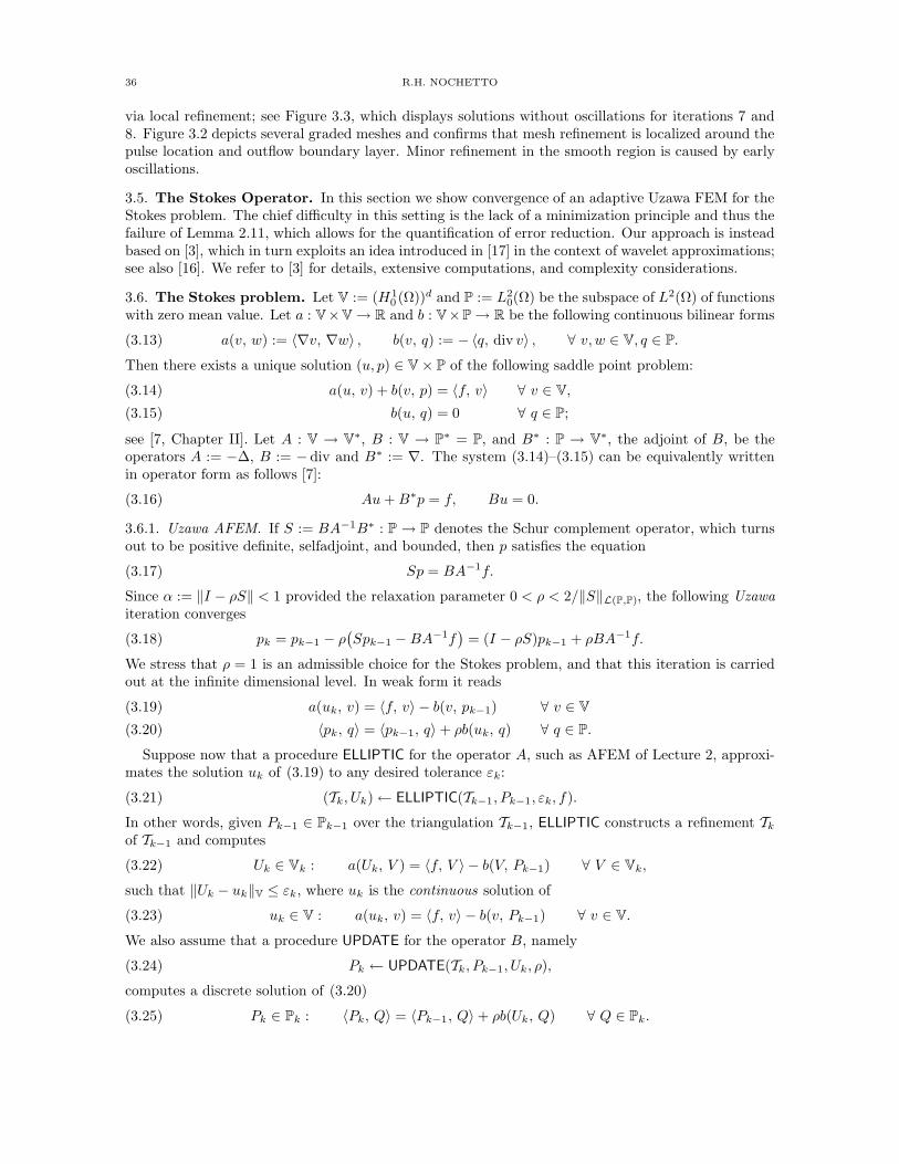
36 R.H. NOCHETTO

via local refinement; see Figure 3.3, which displays solutions without oscillations for iterations 7 and8. Figure 3.2 depicts several graded meshes and confirms that mesh refinement is localized around thepulse location and outflow boundary layer. Minor refinement in the smooth region is caused by earlyoscillations.

3.5. The Stokes Operator. In this section we show convergence of an adaptive Uzawa FEM for theStokes problem. The chief difficulty in this setting is the lack of a minimization principle and thus thefailure of Lemma 2.11, which allows for the quantification of error reduction. Our approach is insteadbased on [3], which in turn exploits an idea introduced in [17] in the context of wavelet approximations;see also [16]. We refer to [3] for details, extensive computations, and complexity considerations.

3.6. The Stokes problem. Let V := (H10 (Ω))d and P := L2

0(Ω) be the subspace of L2(Ω) of functionswith zero mean value. Let a : V×V→ R and b : V×P→ R be the following continuous bilinear forms

(3.13) a(v, w) := 〈∇v, ∇w〉 , b(v, q) := −〈q, div v〉 , ∀ v, w ∈ V, q ∈ P.

Then there exists a unique solution (u, p) ∈ V× P of the following saddle point problem:

a(u, v) + b(v, p) = 〈f, v〉 ∀ v ∈ V,(3.14)

b(u, q) = 0 ∀ q ∈ P;(3.15)

see [7, Chapter II]. Let A : V → V∗, B : V → P

∗ = P, and B∗ : P → V∗, the adjoint of B, be the

operators A := −∆, B := − div and B∗ := ∇. The system (3.14)–(3.15) can be equivalently writtenin operator form as follows [7]:

(3.16) Au + B∗p = f, Bu = 0.

3.6.1. Uzawa AFEM. If S := BA−1B∗ : P → P denotes the Schur complement operator, which turnsout to be positive definite, selfadjoint, and bounded, then p satisfies the equation

(3.17) Sp = BA−1f.

Since α := ‖I − ρS‖ < 1 provided the relaxation parameter 0 < ρ < 2/‖S‖L(P,P), the following Uzawaiteration converges

(3.18) pk = pk−1 − ρ(Spk−1 − BA−1f

)= (I − ρS)pk−1 + ρBA−1f.

We stress that ρ = 1 is an admissible choice for the Stokes problem, and that this iteration is carriedout at the infinite dimensional level. In weak form it reads

a(uk, v) = 〈f, v〉 − b(v, pk−1) ∀ v ∈ V(3.19)

〈pk, q〉 = 〈pk−1, q〉+ ρb(uk, q) ∀ q ∈ P.(3.20)

Suppose now that a procedure ELLIPTIC for the operator A, such as AFEM of Lecture 2, approxi-mates the solution uk of (3.19) to any desired tolerance εk:

(3.21) (Tk, Uk)← ELLIPTIC(Tk−1, Pk−1, εk, f).

In other words, given Pk−1 ∈ Pk−1 over the triangulation Tk−1, ELLIPTIC constructs a refinement Tk

of Tk−1 and computes

(3.22) Uk ∈ Vk : a(Uk, V ) = 〈f, V 〉 − b(V, Pk−1) ∀ V ∈ Vk,

such that ‖Uk − uk‖V ≤ εk, where uk is the continuous solution of

(3.23) uk ∈ V : a(uk, v) = 〈f, v〉 − b(v, Pk−1) ∀ v ∈ V.

We also assume that a procedure UPDATE for the operator B, namely

(3.24) Pk ← UPDATE(Tk, Pk−1, Uk, ρ),

computes a discrete solution of (3.20)

(3.25) Pk ∈ Pk : 〈Pk, Q〉 = 〈Pk−1, Q〉+ ρb(Uk, Q) ∀ Q ∈ Pk.

ADAPTIVE FINITE ELEMENT METHODS FOR ELLIPTIC PDE 37

If Πk : P→ Pk denotes the L2-projection operator, then (3.25) reads equivalently

(3.26) Pk = Pk−1 + ρΠkBUk.

If j is the polynomial degree for velocity, and ` is that for pressure, it turns out that the pairs ofcontinuous finite element spaces

(3.27) Vk = Pj(Tk) ∩ V, Pk = P`(Tk) ∩ P, ` = j, j − 1 ≥ 1,

as well as the discontinuous finite element spaces

(3.28) Vk = Pj(Tk) ∩ V, Pk = Pj−1d (Tk) ∩ P, j ≥ 1,

are of interest. Hereafter, Pjd(Tk) denotes the space of —scalar-valued as well as vector-valued—

(possibly discontinuous) functions that restricted to an element T are polynomials of degree ≤ j for all

T ∈ Tk, and Pj(Tk) denotes the subspace of continuous functions of P jd(Tk). We observe that ` = j−1

in (3.27) corresponds to the popular Taylor-Hood family of finite elements. Any other choice in either(3.27) or (3.28) yields an unstable pair of spaces. These spaces (Vk, Pk) satisfy [3]:

(3.29) ‖ΠkBUk −BUk‖P ≤ C∗εk.

We then have the following convergence result for the Stokes problem, which improves upon theoriginal one in [3].

Theorem 3.10 (Convergence of Uzawa AFEM). Let ρ > 0 be such that α = ‖I − ρS‖ < 1. Givenε0 > 0 and 0 < γ < 1, define εk := γεk−1. Let the procedures ELLIPTIC and UPDATE satisfy (3.22)–(3.26) and (3.29), and let α0 := max(α, γ). Then, for every β such that α0 < β < 1, the iterates(Uk, Pk) ∈ Vk × Pk satisfy

‖p− Pk‖P ≤ Cpβk, ‖u− Uk‖V ≤ Cuβk,

with

Cp := ‖p− P0‖P +ρ(1 + C∗)ε0

β − α0, Cu :=

Cp

β+ ε0.

Proof. In view of (3.22) and (3.26), we see that

Pk = Pk−1 + ρBuk + ρB(Uk − uk) + ρ(Πk − I)BUk

= (I − ρS)Pk−1 + ρBA−1f + ρB(Uk − uk) + ρ(Πk − I)BUk.

Using (3.17), we readily get the error equation

p− Pk = (I − ρS)(p− Pk−1)− ρB(Uk − uk)− ρ(Πk − I)BUk.

We now use the fact that ‖Bv‖P ≤ ‖v‖V for all v ∈ V, and invoke (3.29), to arrive at

‖p− Pk‖P ≤ α‖p− Pk−1‖P + ρ(1 + C∗)εk,

whence, by recursion, we end up with

‖p− Pk‖P ≤ αk‖p− P0‖P + ρ(1 + C∗)ε0

k−1∑

j=0

αjγk−j .

Arguing similarly as in Theorem 2.13, we readily obtain

‖p− Pk‖P ≤ βk(‖p− P0‖P +

ρ(1 + C∗)ε0

β − α0

).

This is the asserted estimate for ‖p− Pk‖P. To obtain a similar bound for ‖u−Uk‖V, we first observethat

a(u− uk, v) = b(v, Pk−1 − p) , ∀v ∈ V,

whence ‖u− uk‖V ≤ ‖p− Pk−1‖P. Since

‖u− Uk‖V ≤ ‖u− uk‖V + ‖uk − Uk‖V ≤ ‖p− Pk−1‖P + εk,

the remaining estimate for ‖u− Uk‖V follows immediately and finishes the proof.

38 R.H. NOCHETTO

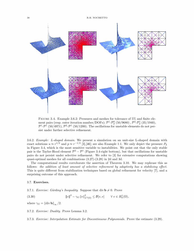
Figure 3.4. Example 3.6.2: Pressures and meshes for tolerance of 5% and finite ele-ment pairs (resp. outer iteration number/DOFs); P1-P0

d (50/9680) , P2-P1d (35/1940),

P1-P1 (50/4971), P2-P1 (50/1200). The oscillations for unstable elements do not per-sist under further selective refinement.

3.6.2. Example: L-shaped domain. We present a simulation on an unit-size L-shaped domain withexact solutions u ≈ r1/2 and p ≈ r−1/2 [3],[46]; see also Example 1.1. We only depict the pressure Pk

in Figure 3.4, which is the most sensitive variable to instabilities. We point out that the only stablepair is the Taylor-Hood element P2 −P1 (Figure 3.4-right bottom), but that oscillations for unstablepairs do not persist under selective refinement. We refer to [3] for extensive computations showingquasi-optimal meshes for all combinations (3.27)-(3.28) in 2d and 3d.

The computational results corroborate the assertion of Theorem 3.10. We may rephrase this asfollows: the addition of least amount of selective refinement by adaptivity has a stabilizing effect.This is quite different from stabilization techniques based on global refinement for velocity [7], and asurprising outcome of this approach.

3.7. Exercises.

3.7.1. Exercise: Garding’s Inequality. Suppose that div b 6= 0. Prove

|||v|||2− γG ‖v‖

2L2(Ω) ≤ B[v, v] ∀ v ∈ H1

0 (Ω),(3.30)

where γG = ‖div b‖∞ /2.

3.7.2. Exercise: Duality. Prove Lemma 3.2.

3.7.3. Exercise: Interpolation Estimate for Discontinuous Polynomials. Prove the estimate (3.29).

ADAPTIVE FINITE ELEMENT METHODS FOR ELLIPTIC PDE 39

3.7.4. Exercise: Complexity of ELLIPTIC. Suppose the tolerance reduction factor γ of Theorem 3.10satisfies γ > α. Show that the number of iterations of ELLIPTIC is bounded by a constant whichdepends only on f , the initial pressure guess P0, the initial triangulation T0, the ratio α/γ, and theparameters θE and θ0 of ELLIPTIC, but on the adaptive counter k.