27-1

Lecture 27

Two-Way ANOVA: Interaction

STAT 512

Spring 2011

Background Reading

KNNL: Chapter 19

27-2

Topic Overview

• Review: Two-way ANOVA Models

• Basic Strategy for Analysis

• Studying Interactions

27-3

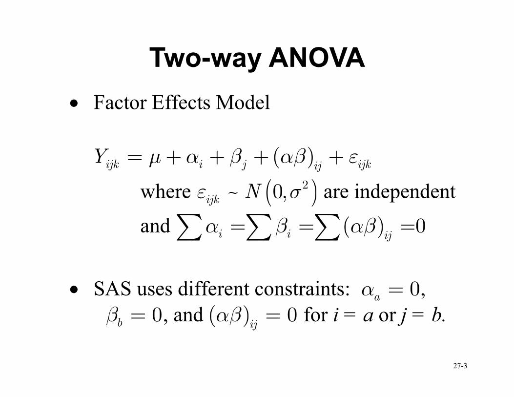
Two-way ANOVA

• Factor Effects Model

( )ijk i j ijkijY µ α β αβ ε= + + + +

where ( )2~ 0,ijk Nε σ are independent

and ( ) 0i i ijα β αβ= = =∑ ∑ ∑

• SAS uses different constraints: 0aα = ,

0bβ = , and ( ) 0ij

αβ = for i = a or j = b.

27-4

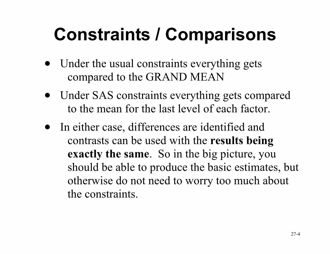
Constraints / Comparisons

• Under the usual constraints everything gets

compared to the GRAND MEAN

• Under SAS constraints everything gets compared

to the mean for the last level of each factor.

• In either case, differences are identified and

contrasts can be used with the results being

exactly the same. So in the big picture, you

should be able to produce the basic estimates, but

otherwise do not need to worry too much about

the constraints.

27-5

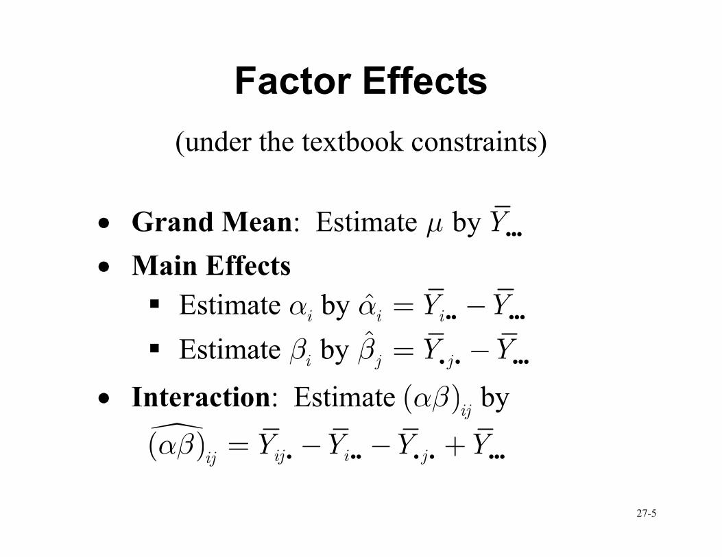
Factor Effects

(under the textbook constraints)

• Grand Mean: Estimate µ by Yiii

• Main Effects

� Estimate iα by i iY Yα = −ii iii

� Estimate iβ by ˆj jY Yβ = −

i i iii

• Interaction: Estimate ( )ij

αβ by

( )� ij i jijY Y Y Yαβ = − − +i ii i i iii

27-6

General Strategy for Multiple ANOVA Analysis

• Every thing we are doing can be extended to

any number of variables.

• We will now consider a general strategy for

approaching this type of data.

27-7

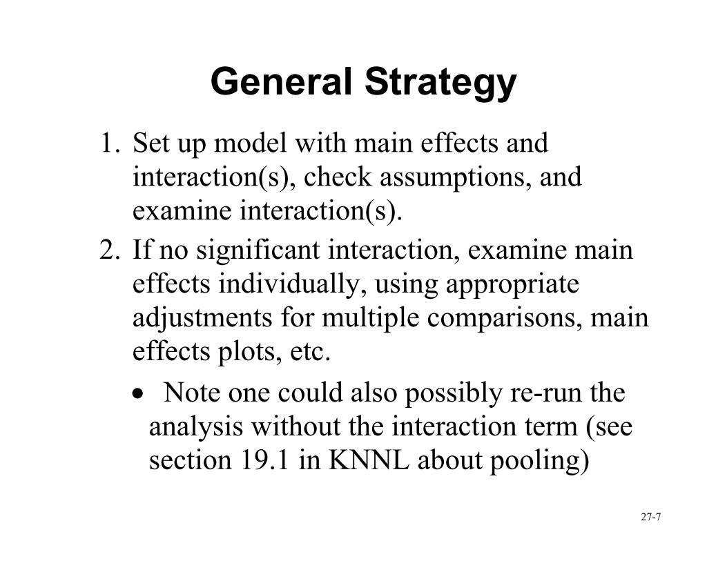
General Strategy

1. Set up model with main effects and

interaction(s), check assumptions, and

examine interaction(s).

2. If no significant interaction, examine main

effects individually, using appropriate

adjustments for multiple comparisons, main

effects plots, etc.

• Note one could also possibly re-run the

analysis without the interaction term (see

section 19.1 in KNNL about pooling)

27-8

Analysis Strategies (2)

3. If interaction is significant, determine

whether interactions are important. If not,

can examine main effects as in Step 2.

4. If interaction present & important, determine

whether interaction is simple or complex.

5. For simple interactions, can still talk about

the main effects of A at each level of B

6. For complex interaction, must simply

consider all pairs of levels as separate

treatments.

27-9

Unimportant Interactions

• If interaction effects are very small

compared to main effects or only apparent

in a small number of treatments, then they

are probably unimportant.

• Lines will be not quite parallel, but close.

• We can proceed by keeping interaction in

the model, but using marginal means for

each significant main effect individually

• Marginal means: Averages over the levels

of the other factor.

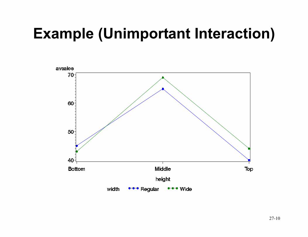
27-10

Example (Unimportant Interaction)

27-11

Important Interactions

• The interaction effect is so large and/or

pervasive that main effects cannot be

interpreted on their own.

• In interaction plots, the lines will not be

parallel. They may or may not criss-cross,

but the differences between levels for one

factor will depend on the level of the other

factor

27-12

Important Interactions

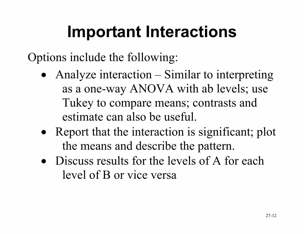
Options include the following:

• Analyze interaction – Similar to interpreting

as a one-way ANOVA with ab levels; use

Tukey to compare means; contrasts and

estimate can also be useful.

• Report that the interaction is significant; plot

the means and describe the pattern.

• Discuss results for the levels of A for each

level of B or vice versa

27-13

Simple vs. Complex Interactions

• An interaction is considered simple if we

can discuss trends for the main effect of

one factor for each level of the other factor,

and if the general trend is the same.

• An interaction is complex if it is difficult to

discuss anything about the main effects. In

this situation, one can only look at

treatment combinations and cannot

separate them into main effects easily.

27-14

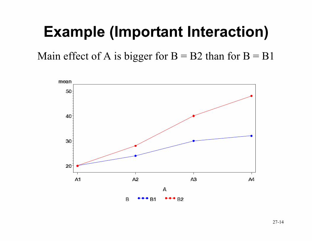
Example (Important Interaction)

Main effect of A is bigger for B = B2 than for B = B1

27-15

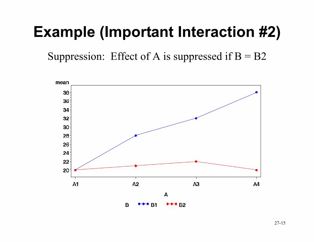
Example (Important Interaction #2)

Suppression: Effect of A is suppressed if B = B2

27-16

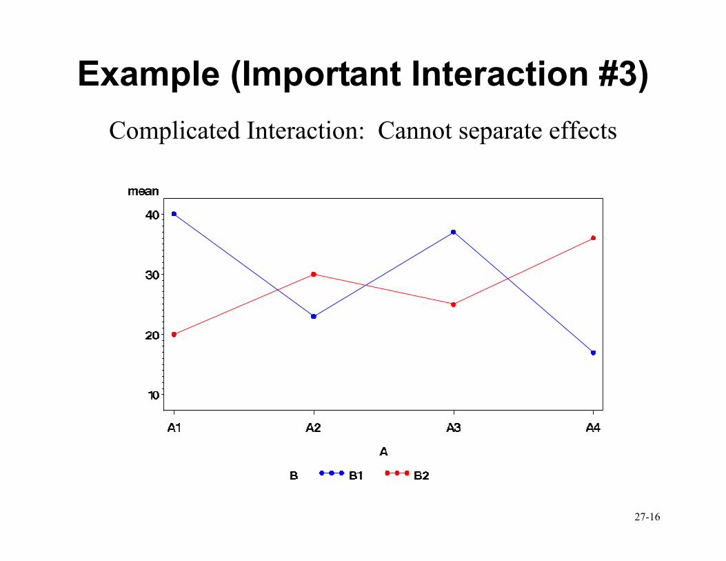
Example (Important Interaction #3)

Complicated Interaction: Cannot separate effects

27-17

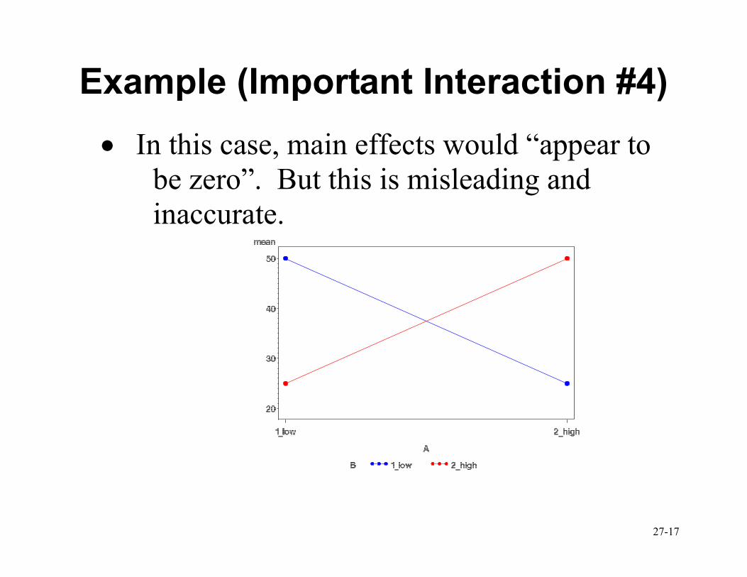
Example (Important Interaction #4)

• In this case, main effects would “appear to

be zero”. But this is misleading and

inaccurate.

27-18

Example (Important Interaction #4)

• If you averaged over either factor, you

would find “no change” when going from

one level to the other.

• In fact there is a change when going from

one level to the next, and the type of

change depends on the level of the second

factor. (This is a good “definition” for

interaction.)

27-19

Example (Important Interaction #4)

Conclusions should be...

• At the low level of factor B, increasing A

from low to high decreases the mean

response.

• At the high level of factor B, increasing A

from low to high increases the mean

response.

• You cannot make statements here about

Factor A alone or Factor B alone.

27-20

Battery Example

• Study the effects of A = type of material and B

= temperature on the lifetime of a battery (in

hours).

• Three material types (experimental) – Nickel-

Cadmium, Nickel-Metal Hydride, and

Lithium-Ion

• Three temperatures (also experimental) – 15,

70, and 125 degrees Fahrenheit

27-21

Battery Example (2)

• Four observations per cell

• Goal is to examine the effects and hopefully

find a material that will help the battery have

a uniformly long life in the field.

• Steps in analysis:

� Check interaction plot

� Review ANOVA results / assumptions

� Check main effects if appropriate

� Draw conclusions

27-22

Interaction

27-23

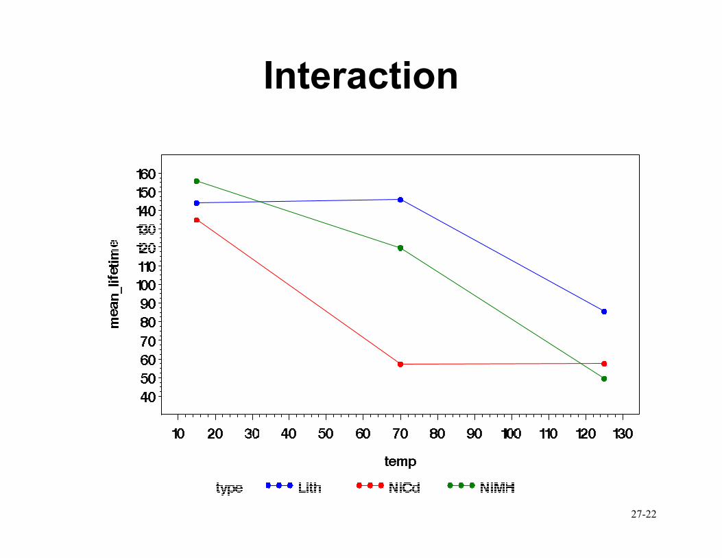
Interaction (2)

• Interaction here is complicated but quite

informative.

• It appears the Ni-Cd battery is “worst” – we

would want to eliminate that from production

if the costs were all the same.

• We’ll take a look at the rest in greater detail,

but the plot makes us suspect the Lithium ion

battery is superior.

27-24

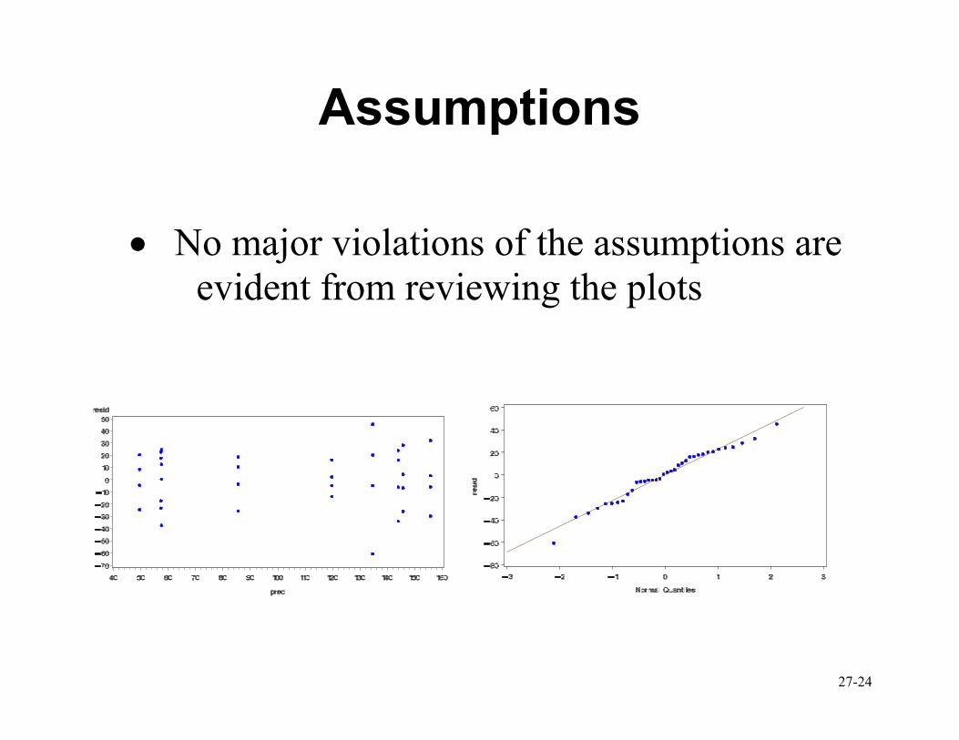
Assumptions

• No major violations of the assumptions are

evident from reviewing the plots

27-25

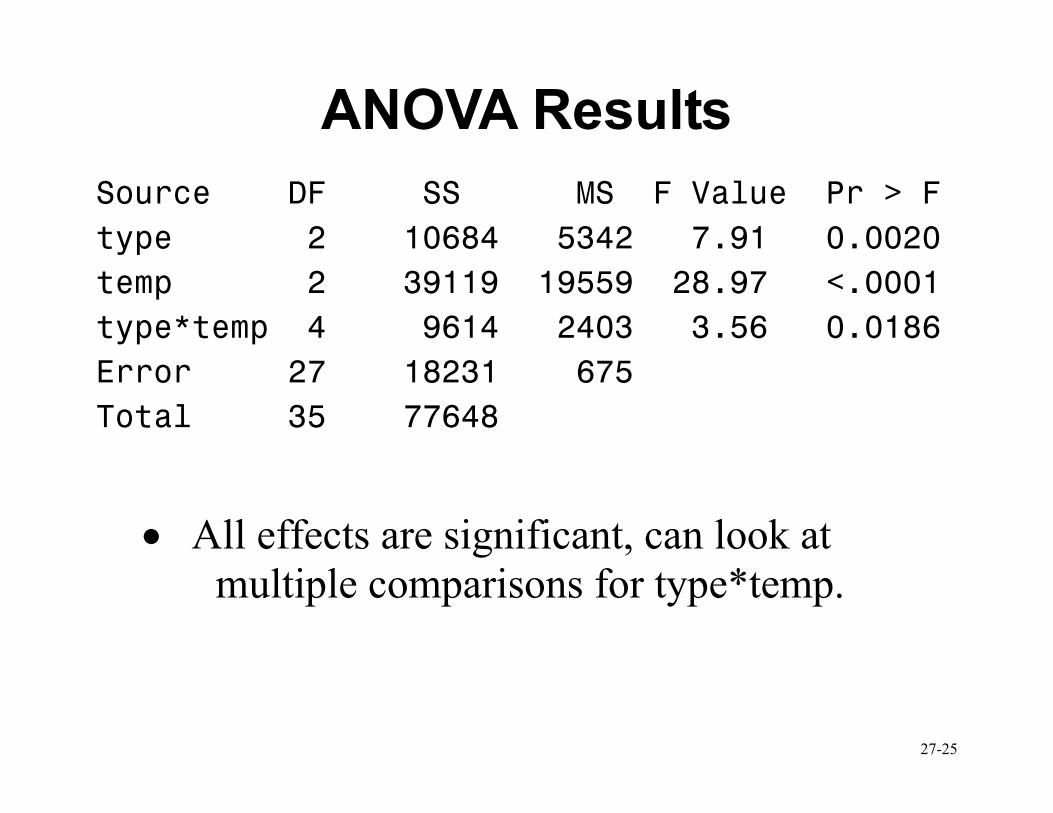
ANOVA Results

Source DF SS MS F Value Pr > F

type 2 10684 5342 7.91 0.0020

temp 2 39119 19559 28.97 <.0001

type*temp 4 9614 2403 3.56 0.0186

Error 27 18231 675

Total 35 77648

• All effects are significant, can look at

multiple comparisons for type*temp.

27-26

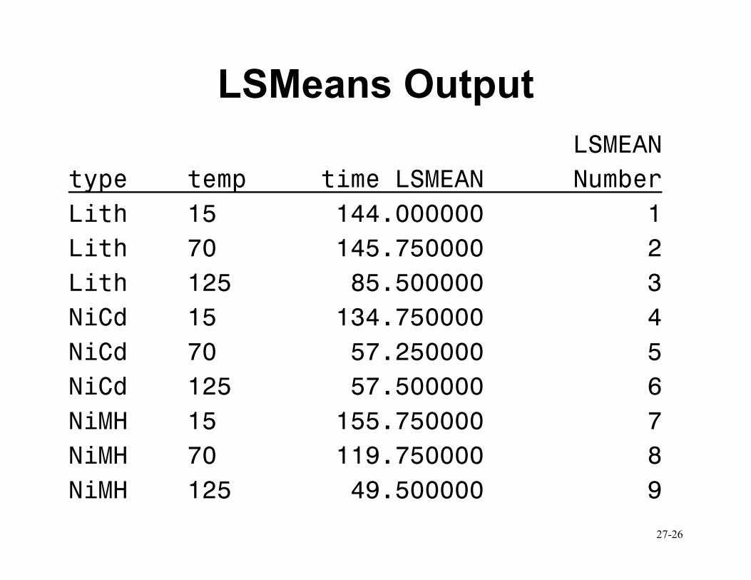
LSMeans Output

LSMEAN

type temp time LSMEAN Number

Lith 15 144.000000 1

Lith 70 145.750000 2

Lith 125 85.500000 3

NiCd 15 134.750000 4

NiCd 70 57.250000 5

NiCd 125 57.500000 6

NiMH 15 155.750000 7

NiMH 70 119.750000 8

NiMH 125 49.500000 9

27-27

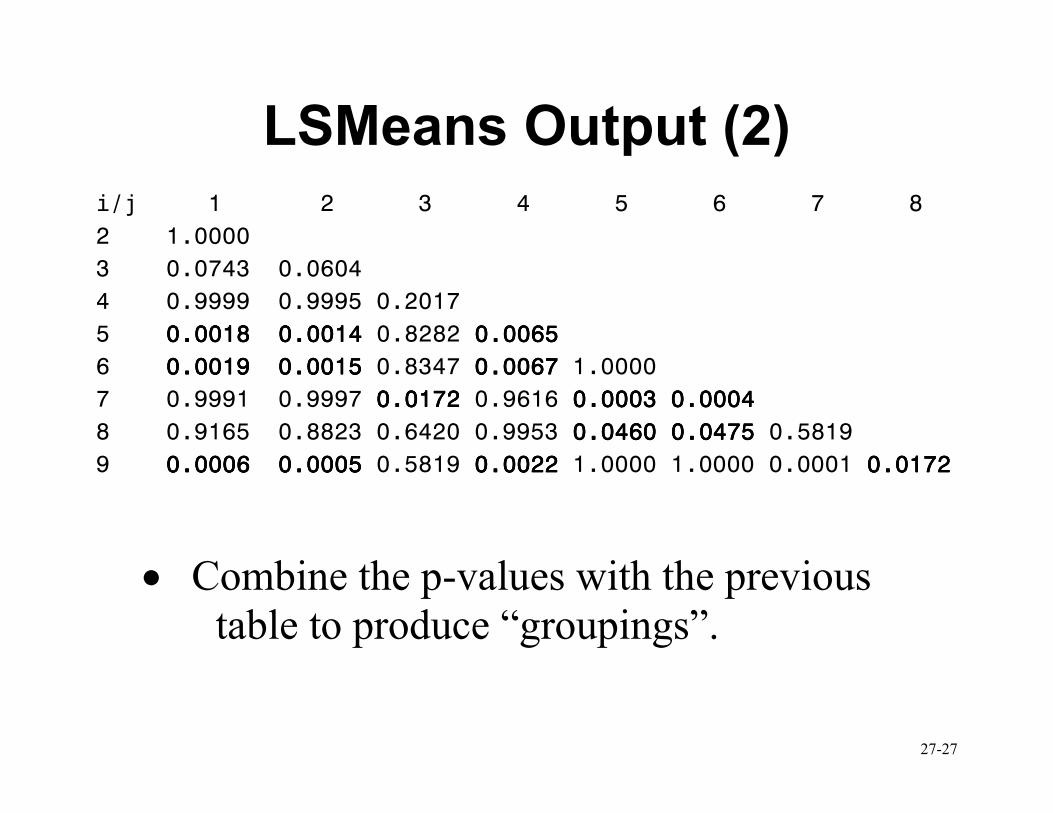
LSMeans Output (2)

i/j 1 2 3 4 5 6 7 8

2 1.0000

3 0.0743 0.0604

4 0.9999 0.9995 0.2017

5 0.0018 0.0014 0.0018 0.0014 0.0018 0.0014 0.0018 0.0014 0.8282 0.00650.00650.00650.0065

6 0.00190.00190.00190.0019 0.00150.00150.00150.0015 0.8347 0.00670.00670.00670.0067 1.0000

7 0.9991 0.9997 0.01720.01720.01720.0172 0.9616 0.00030.00030.00030.0003 0.00040.00040.00040.0004

8 0.9165 0.8823 0.6420 0.9953 0.0460 0.04750.0460 0.04750.0460 0.04750.0460 0.0475 0.5819

9 0.00060.00060.00060.0006 0.00050.00050.00050.0005 0.5819 0.00220.00220.00220.0022 1.0000 1.0000 0.0001 0.01720.01720.01720.0172

• Combine the p-values with the previous

table to produce “groupings”.

27-28

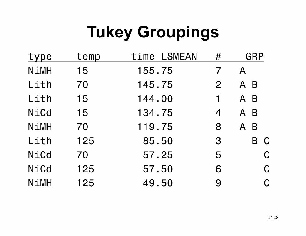
Tukey Groupings

type temp time LSMEAN # GRP

NiMH 15 155.75 7 A

Lith 70 145.75 2 A B

Lith 15 144.00 1 A B

NiCd 15 134.75 4 A B

NiMH 70 119.75 8 A B

Lith 125 85.50 3 B C

NiCd 70 57.25 5 C

NiCd 125 57.50 6 C

NiMH 125 49.50 9 C

27-29

Conclusions

• At 15 degrees there is no significant diff.

• At 70 degrees Lithium-ion or Nickel-MH

are significantly different from Ni-Cd

• At 125 degrees there was no significant diff.

• If we had a little more power, we might be

able to show that the Lithium-ion battery

was best at 70 or 125 degrees, and

equivalent to the others 15 degrees.

• Further testing with more observations

might be useful.

27-30

Upcoming in Lecture 28...

• Additive Models

• One Case per Treatment

• Unequal Sample Sizes