Lecture 23: Neural Networks - Department of Statistics

Lecture 23: Neural Networks

Wenbin Lu

Department of StatisticsNorth Carolina State University

Fall 2019

Wenbin Lu (NCSU) Data Mining and Machine Learning Fall 2019 1 / 30

Outlines

Projection Pursuit Regression (PPR)

Neural Network

Deep Neural Network (DNN)

Convolutional Neural Networks (CNN)

Recurrent Neural Networks (RNN)

Generative Adversarial Networks (GAN)


Projection Pursuit Regression

Projection Pursuit Regression (PPR)

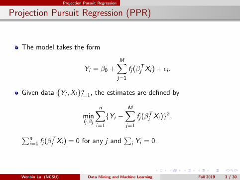
The model takes the form

Yi = β0 +M∑j=1

fj(βTj Xi ) + εi .

Given data Yi ,Xini=1, the estimates are defined by

minfj ,βj

n∑i=1

Yi −M∑j=1

fj(βTj Xi )2,

∑ni=1 fj(β

Tj Xi ) = 0 for any j and

∑i Yi = 0.


Projection Pursuit Regression

Computation

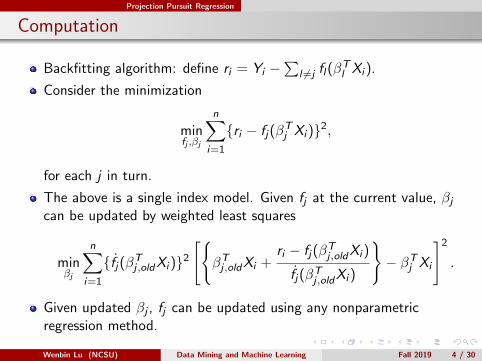
Backfitting algorithm: define ri = Yi −∑

l 6=j fl(βTl Xi ).

Consider the minimization

minfj ,βj

n∑i=1

ri − fj(βTj Xi )2,

for each j in turn.

The above is a single index model. Given fj at the current value, βjcan be updated by weighted least squares

minβj

n∑i=1

fj(βTj ,oldXi )2[

βTj ,oldXi +ri − fj(β

Tj ,oldXi )

fj(βTj ,oldXi )

− βTj Xi

]2

.

Given updated βj , fj can be updated using any nonparametricregression method.


Neural Networks

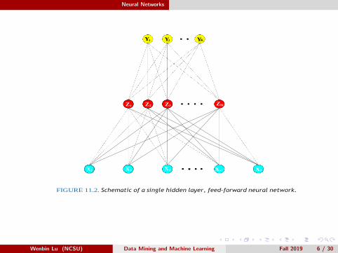
Single Layer Neural Networks

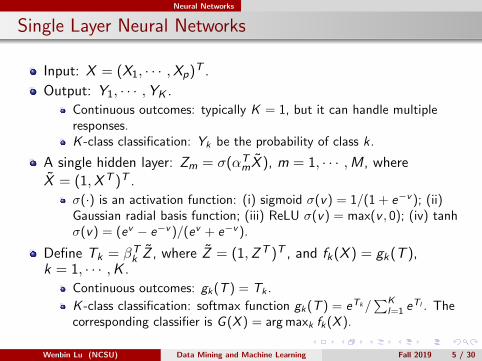
Input: X = (X1, · · · ,Xp)T .

Output: Y1, · · · ,YK .

Continuous outcomes: typically K = 1, but it can handle multipleresponses.K -class classification: Yk be the probability of class k.

A single hidden layer: Zm = σ(αTmX ), m = 1, · · · ,M, where

X = (1,XT )T .

σ(·) is an activation function: (i) sigmoid σ(v) = 1/(1 + e−v ); (ii)Gaussian radial basis function; (iii) ReLU σ(v) = max(v , 0); (iv) tanhσ(v) = (ev − e−v )/(ev + e−v ).

Define Tk = βTk Z , where Z = (1,ZT )T , and fk(X ) = gk(T ),k = 1, · · · ,K .

Continuous outcomes: gk(T ) = Tk .

K -class classification: softmax function gk(T ) = eTk/∑K

l=1 eTl . The

corresponding classifier is G (X ) = arg maxk fk(X ).


Neural Networks

FIGURE 11.2. Schematic of a single hidden layer, feed-forward neural network.

Y1 Y2 YK

Z1 Z2 Z3 ZM

X1 X2 X3 Xp-1 Xp


Neural Networks

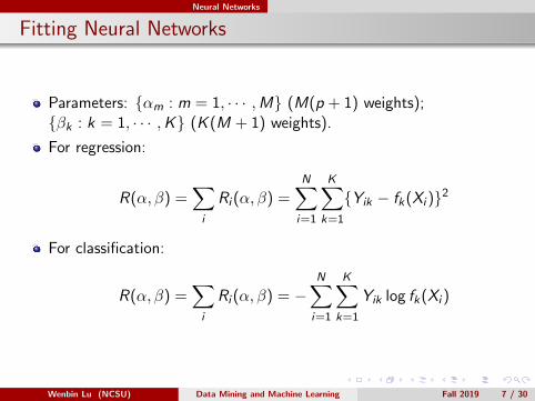
Fitting Neural Networks

Parameters: αm : m = 1, · · · ,M (M(p + 1) weights);βk : k = 1, · · · ,K (K (M + 1) weights).

For regression:

R(α, β) =∑i

Ri (α, β) =N∑i=1

K∑k=1

Yik − fk(Xi )2

For classification:

R(α, β) =∑i

Ri (α, β) = −N∑i=1

K∑k=1

Yik log fk(Xi )


Neural Networks

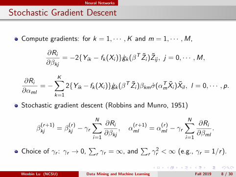
Stochastic Gradient Descent

Compute gradients: for k = 1, · · · ,K and m = 1, · · · ,M,

∂Ri

∂βkj= −2Yik − fk(Xi )gk(βT Zi )Zij , j = 0, · · · ,M,

∂Ri

∂αml= −

K∑k=1

2Yik − fk(Xi )gk(βT Zi )βkmσ(αTmXi )Xil , l = 0, · · · , p.

Stochastic gradient descent (Robbins and Munro, 1951)

β(r+1)kj = β

(r)kj − γr

N∑i=1

∂Ri

∂βkj, α

(r+1)ml = α

(r)ml − γr

N∑i=1

∂Ri

∂βml.

Choice of γr : γr → 0,∑

r γr =∞, and∑

r γ2r <∞ (e.g., γr = 1/r).


Neural Networks

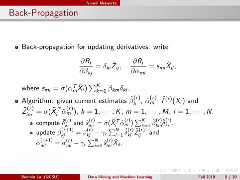
Back-Propagation

Back-propagation for updating derivatives: write

∂Ri

∂βkj= δki Zij ,

∂Ri

∂αml= smi Xil ,

where smi = σ(αTmXi )

∑Kk=1 βkmδki .

Algorithm: given current estimates β(r)k , α

(r)m , f (r)(Xi ) and

Z(r)im = σ(XT

i α(r)m ), k = 1, · · · ,K , m = 1, · · · ,M, i = 1, · · · ,N.

compute δ(r)ki and s

(r)mi = σ(XT

i α(r)m )

∑Kk=1 β

(r)kmδ

(r)ki .

update β(r+1)kj = β

(r)kj − γr

∑Ni=1 δ

(r)ki Z

(r)ij , and

α(r+1)ml = α

(r)ml − γr

∑Ni=1 s

(r)mi Xil .


Deep Neural Networks



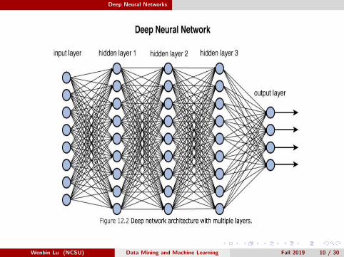
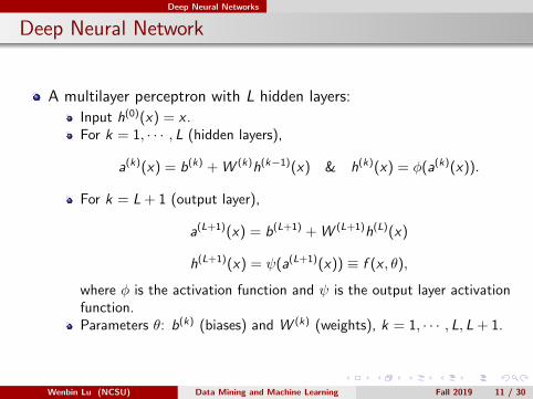
Deep Neural Network

A multilayer perceptron with L hidden layers:

Input h(0)(x) = x .For k = 1, · · · , L (hidden layers),

a(k)(x) = b(k) + W (k)h(k−1)(x) & h(k)(x) = φ(a(k)(x)).

For k = L + 1 (output layer),

a(L+1)(x) = b(L+1) + W (L+1)h(L)(x)

h(L+1)(x) = ψ(a(L+1)(x)) ≡ f (x , θ),

where φ is the activation function and ψ is the output layer activationfunction.Parameters θ: b(k) (biases) and W (k) (weights), k = 1, · · · , L, L + 1.



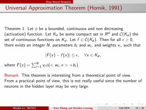
Universal Approximation Theorem (Hornik, 1991)

Theorem 1. Let φ be a bounded, continuous and non decreasing(activation) function. Let Kd be some compact set in Rd and C(Kd) theset of continuous functions on Kd . Let f ∈ C(Kd). Then for all ε > 0,there exists an integer N, parameters bi and wi , and weights vi , such that

|F (x)− f (x)| ≤ ε, ∀x ∈ Kd ,

where F (x) =∑N

i=1 viφ(< wi , x > +bi ).

Remark: This theorem is interesting from a theoretical point of view.From a practical point of view, this is not really useful since the number ofneurons in the hidden layer may be very large.



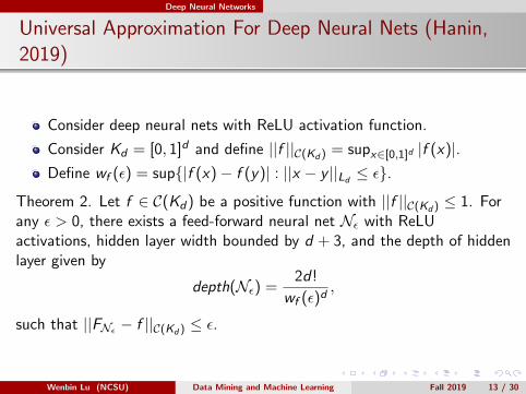
Universal Approximation For Deep Neural Nets (Hanin,2019)

Consider deep neural nets with ReLU activation function.

Consider Kd = [0, 1]d and define ||f ||C(Kd ) = supx∈[0,1]d |f (x)|.Define wf (ε) = sup|f (x)− f (y)| : ||x − y ||Ld ≤ ε.

Theorem 2. Let f ∈ C(Kd) be a positive function with ||f ||C(Kd ) ≤ 1. Forany ε > 0, there exists a feed-forward neural net Nε with ReLUactivations, hidden layer width bounded by d + 3, and the depth of hiddenlayer given by

depth(Nε) =2d!

wf (ε)d,

such that ||FNε − f ||C(Kd ) ≤ ε.



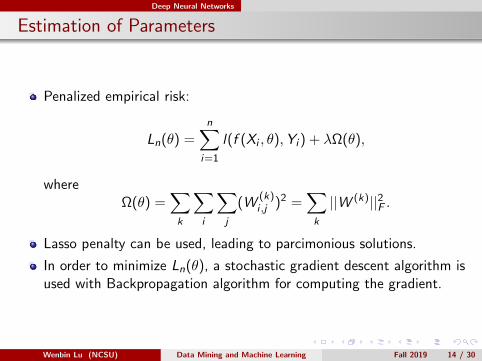
Estimation of Parameters

Penalized empirical risk:

Ln(θ) =n∑

i=1

l(f (Xi , θ),Yi ) + λΩ(θ),

whereΩ(θ) =

∑k

∑i

∑j

(W(k)i ,j )2 =

∑k

||W (k)||2F .

Lasso penalty can be used, leading to parcimonious solutions.

In order to minimize Ln(θ), a stochastic gradient descent algorithm isused with Backpropagation algorithm for computing the gradient.



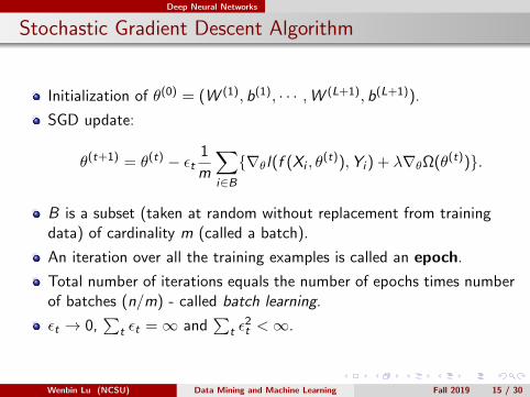
Stochastic Gradient Descent Algorithm

Initialization of θ(0) = (W (1), b(1), · · · ,W (L+1), b(L+1)).

SGD update:

θ(t+1) = θ(t) − εt1

m

∑i∈B∇θl(f (Xi , θ

(t)),Yi ) + λ∇θΩ(θ(t)).

B is a subset (taken at random without replacement from trainingdata) of cardinality m (called a batch).

An iteration over all the training examples is called an epoch.

Total number of iterations equals the number of epochs times numberof batches (n/m) - called batch learning.

εt → 0,∑

t εt =∞ and∑

t ε2t <∞.



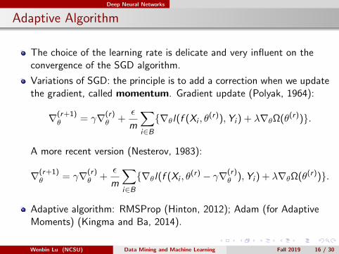
Adaptive Algorithm

The choice of the learning rate is delicate and very influent on theconvergence of the SGD algorithm.

Variations of SGD: the principle is to add a correction when we updatethe gradient, called momentum. Gradient update (Polyak, 1964):

∇(r+1)θ = γ∇(r)

θ +ε

m


(r)),Yi ) + λ∇θΩ(θ(r)).

A more recent version (Nesterov, 1983):

∇(r+1)θ = γ∇(r)

θ +ε

m


(r) − γ∇(r)θ ),Yi ) + λ∇θΩ(θ(r)).

Adaptive algorithm: RMSProp (Hinton, 2012); Adam (for AdaptiveMoments) (Kingma and Ba, 2014).



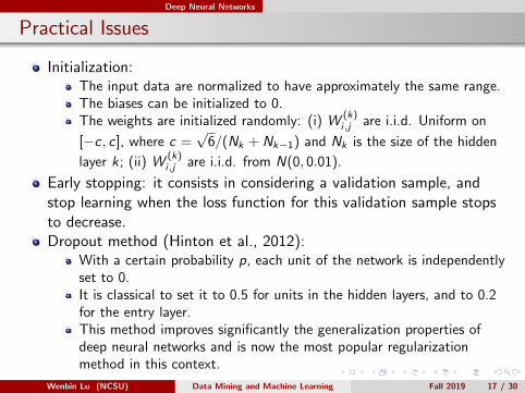
Practical Issues

Initialization:The input data are normalized to have approximately the same range.The biases can be initialized to 0.The weights are initialized randomly: (i) W

(k)i,j are i.i.d. Uniform on

[−c , c], where c =√

6/(Nk + Nk−1) and Nk is the size of the hidden

layer k ; (ii) W(k)i,j are i.i.d. from N(0, 0.01).

Early stopping: it consists in considering a validation sample, andstop learning when the loss function for this validation sample stopsto decrease.Dropout method (Hinton et al., 2012):

With a certain probability p, each unit of the network is independentlyset to 0.It is classical to set it to 0.5 for units in the hidden layers, and to 0.2for the entry layer.This method improves significantly the generalization properties ofdeep neural networks and is now the most popular regularizationmethod in this context.


Convolutional Neural Networks


Multilayer perceptrons are defined for vectors as input data; not welladapted some types of data, such as images.

Transforming the images into vectors may loose by the way thespatial informations contained in the images.

Old image processing (before deep learning): extraction of variablesof interest, called features.

Convolutional neural networks (CNN): introduced by LeCun et al.(1998); have revolutionized image processing; widely used for imageclassification, image segmentation, object recognition, facerecognition.



Layers in a CNN

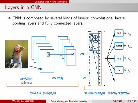
CNN is composed by several kinds of layers: convolutional layers,pooling layers and fully connected layers.



Convolutional Layers

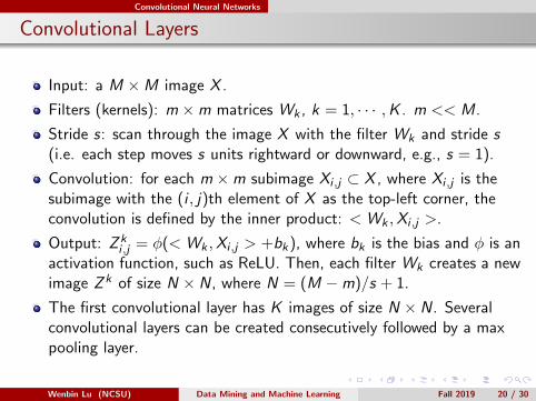
Input: a M ×M image X .

Filters (kernels): m ×m matrices Wk , k = 1, · · · ,K . m << M.

Stride s: scan through the image X with the filter Wk and stride s(i.e. each step moves s units rightward or downward, e.g., s = 1).

Convolution: for each m ×m subimage Xi ,j ⊂ X , where Xi ,j is thesubimage with the (i , j)th element of X as the top-left corner, theconvolution is defined by the inner product: <Wk ,Xi ,j >.

Output: Z ki ,j = φ(<Wk ,Xi ,j > +bk), where bk is the bias and φ is an

activation function, such as ReLU. Then, each filter Wk creates a newimage Z k of size N × N, where N = (M −m)/s + 1.

The first convolutional layer has K images of size N × N. Severalconvolutional layers can be created consecutively followed by a maxpooling layer.



Pooling Layers

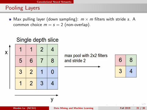
Max pulling layer (down sampling): m ×m filters with stride s. Acommon choice m = s = 2 (non-overlap).



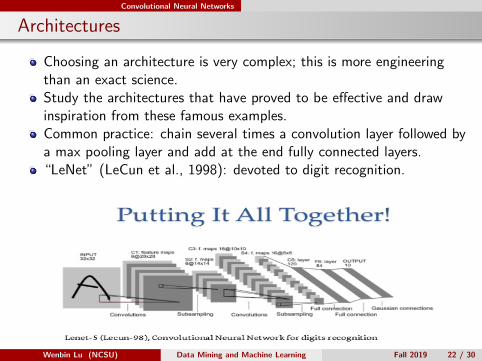
Architectures

Choosing an architecture is very complex; this is more engineeringthan an exact science.Study the architectures that have proved to be effective and drawinspiration from these famous examples.Common practice: chain several times a convolution layer followed bya max pooling layer and add at the end fully connected layers.“LeNet” (LeCun et al., 1998): devoted to digit recognition.



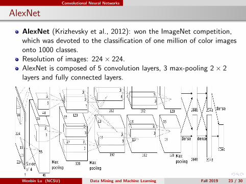
AlexNet

AlexNet (Krizhevsky et al., 2012): won the ImageNet competition,which was devoted to the classification of one million of color imagesonto 1000 classes.Resolution of images: 224× 224.AlexNet is composed of 5 convolution layers, 3 max-pooling 2× 2layers and fully connected layers.



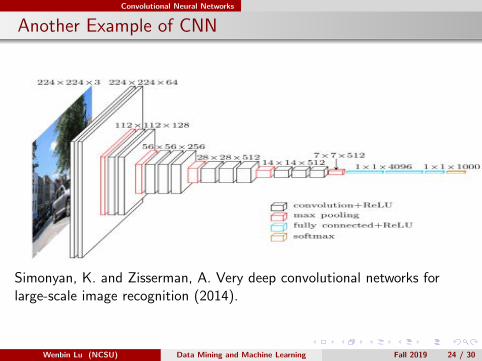
Another Example of CNN

Simonyan, K. and Zisserman, A. Very deep convolutional networks forlarge-scale image recognition (2014).



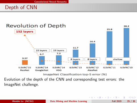
Depth of CNN

Evolution of the depth of the CNN and corresponding test errors: theImageNet challenge.


Recurrent Neural Networks


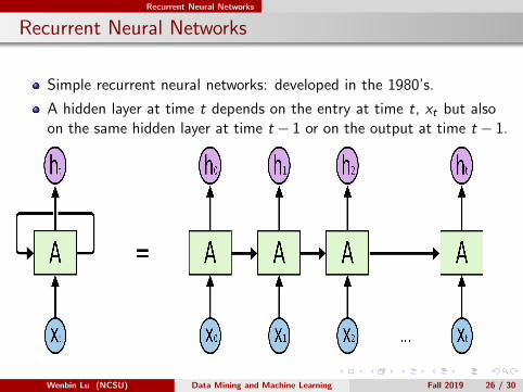
Simple recurrent neural networks: developed in the 1980’s.

A hidden layer at time t depends on the entry at time t, xt but alsoon the same hidden layer at time t − 1 or on the output at time t − 1.



Long Short-Term Memory (LSTM)

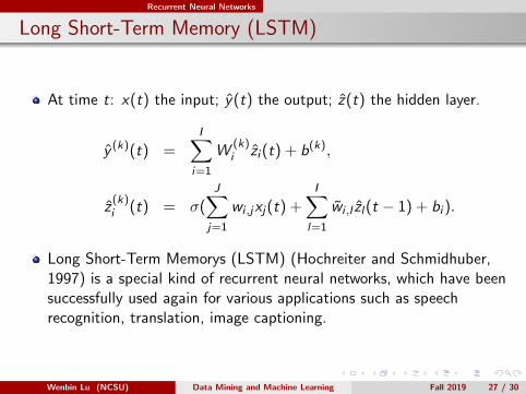
At time t: x(t) the input; y(t) the output; z(t) the hidden layer.

y (k)(t) =I∑

i=1

W(k)i zi (t) + b(k),

z(k)i (t) = σ(

J∑j=1

wi ,jxj(t) +I∑

l=1

wi ,l zl(t − 1) + bi ).

Long Short-Term Memorys (LSTM) (Hochreiter and Schmidhuber,1997) is a special kind of recurrent neural networks, which have beensuccessfully used again for various applications such as speechrecognition, translation, image captioning.


Generative Adversarial Networks

Generative Adversarial Networks(GAN)

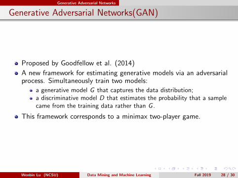
Proposed by Goodfellow et al. (2014)

A new framework for estimating generative models via an adversarialprocess. Simultaneously train two models:

a generative model G that captures the data distribution;a discriminative model D that estimates the probability that a samplecame from the training data rather than G .

This framework corresponds to a minimax two-player game.



Adversarial Nets

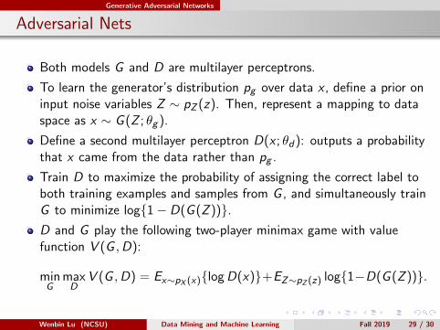
Both models G and D are multilayer perceptrons.

To learn the generator’s distribution pg over data x , define a prior oninput noise variables Z ∼ pZ (z). Then, represent a mapping to dataspace as x ∼ G (Z ; θg ).

Define a second multilayer perceptron D(x ; θd): outputs a probabilitythat x came from the data rather than pg .

Train D to maximize the probability of assigning the correct label toboth training examples and samples from G , and simultaneously trainG to minimize log1− D(G (Z )).D and G play the following two-player minimax game with valuefunction V (G ,D):

minG

maxD

V (G ,D) = Ex∼pX (x)logD(x)+EZ∼pZ (z) log1−D(G (Z )).



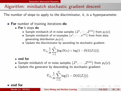
Algorithm: minibatch stochastic gradient descent

The number of steps to apply to the discriminator, k , is a hyperparameter.

For number of training iterations doFor k steps do

Sample minibatch of m noise samples Z 1, · · · ,Z (m) from pZ (z).Sample minibatch of m examples x1, · · · , x (m) from from datagenerating distribution pX (x).Update the discriminator by ascending its stochastic gradient:

∇θd

1

m

m∑i=1

[logD(xi ) + log1− D(G(Zi ))] .

end forSample minibatch of m noise samples Z 1, · · · ,Z (m) from pZ (z).Update the generator by descending its stochastic gradient:

∇θg1

m

m∑i=1

log1− D(G (Zi )).

end forWenbin Lu (NCSU) Data Mining and Machine Learning Fall 2019 30 / 30

Lecture 23: Neural Networks - Department of Statistics

Documents

Transcript of Lecture 23: Neural Networks - Department of Statistics