L. Vandenberghe EE236A (Fall 2013-14)

Lecture 2Piecewise-linear optimization

• piecewise-linear minimization

• ℓ1- and ℓ∞-norm approximation

• examples

• modeling software

2–1

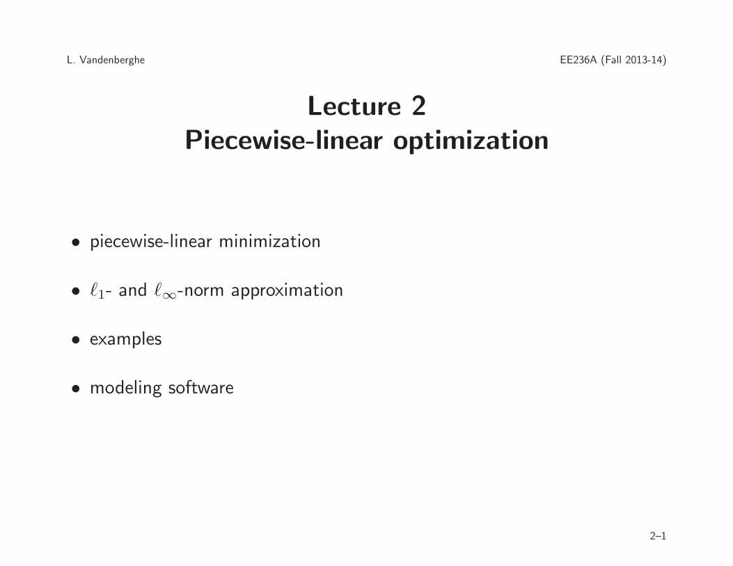
Linear and affine functions

linear function: a function f : Rn → R is linear if

f(αx+ βy) = αf(x) + βf(y) ∀x, y ∈ Rn, α, β ∈ R

property: f is linear if and only if f(x) = aTx for some a

affine function: a function f : Rn → R is affine if

f(αx+ (1− α)y) = αf(x) + (1− α)f(y) ∀x, y ∈ Rn, α ∈ R

property: f is affine if and only if f(x) = aTx+ b for some a, b

Piecewise-linear optimization 2–2

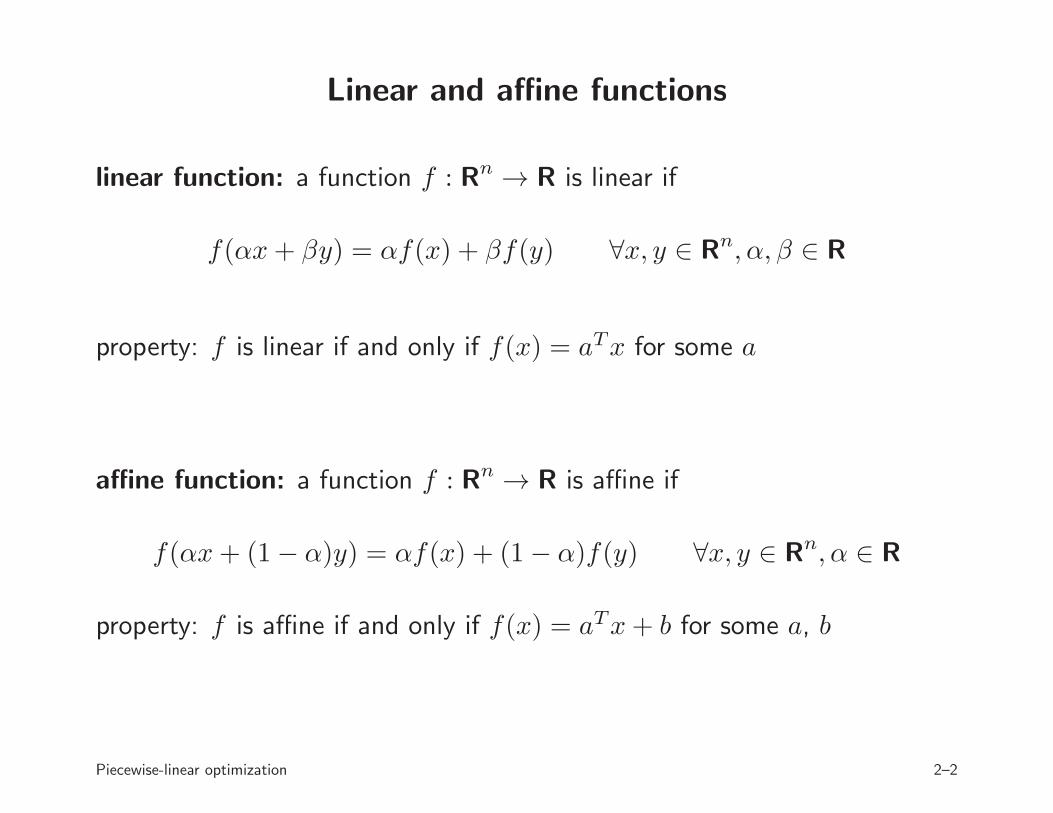
Piecewise-linear function

f : Rn → R is (convex) piecewise-linear if it can be expressed as

f(x) = maxi=1,...,m

(aTi x+ bi)

f is parameterized by m n-vectors ai and m scalars bi

x

aTi x + bi

f(x)

(the term piecewise-affine is more accurate but less common)

Piecewise-linear optimization 2–3

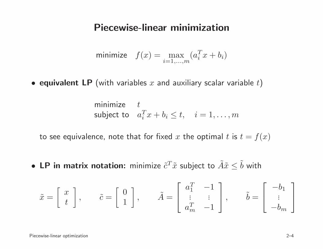
Piecewise-linear minimization

minimize f(x) = maxi=1,...,m

(aTi x+ bi)

• equivalent LP (with variables x and auxiliary scalar variable t)

minimize tsubject to aTi x+ bi ≤ t, i = 1, . . . ,m

to see equivalence, note that for fixed x the optimal t is t = f(x)

• LP in matrix notation: minimize cT x subject to Ax ≤ b with

x =

[

xt

]

, c =

[

01

]

, A =

aT1 −1... ...aTm −1

, b =

−b1...

−bm

Piecewise-linear optimization 2–4

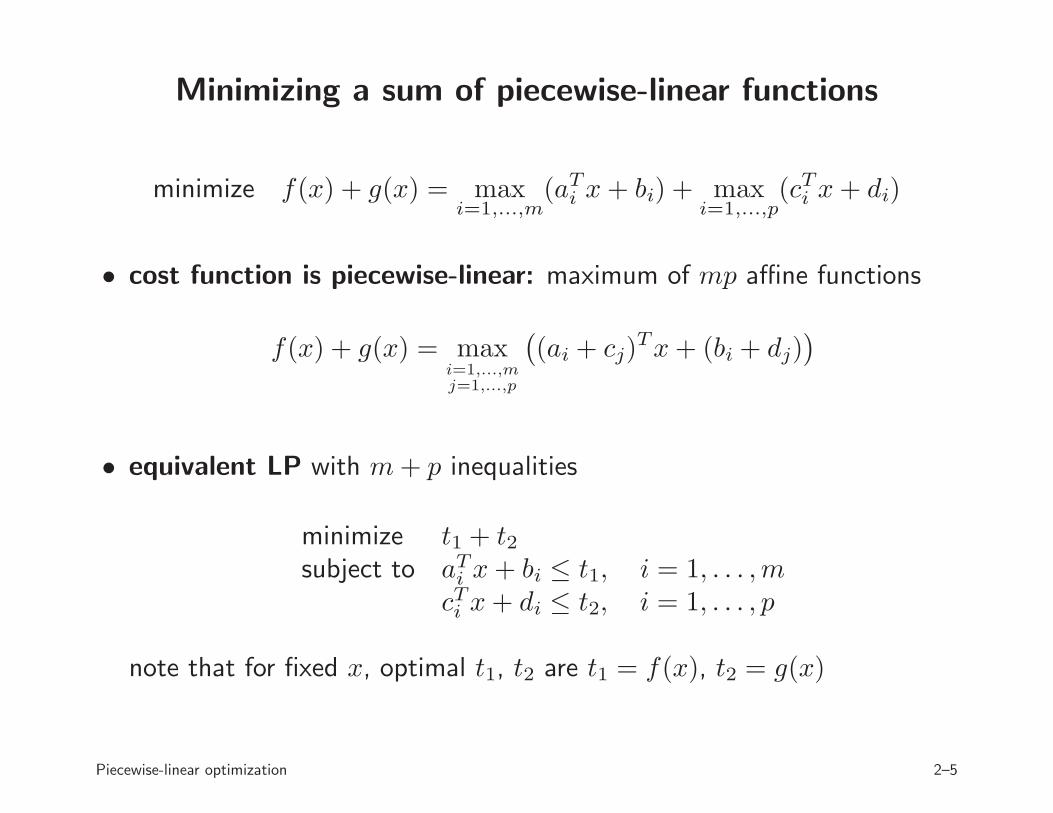
Minimizing a sum of piecewise-linear functions

minimize f(x) + g(x) = maxi=1,...,m

(aTi x+ bi) + maxi=1,...,p

(cTi x+ di)

• cost function is piecewise-linear: maximum of mp affine functions

f(x) + g(x) = maxi=1,...,mj=1,...,p

(

(ai + cj)Tx+ (bi + dj)

)

• equivalent LP with m+ p inequalities

minimize t1 + t2subject to aTi x+ bi ≤ t1, i = 1, . . . ,m

cTi x+ di ≤ t2, i = 1, . . . , p

note that for fixed x, optimal t1, t2 are t1 = f(x), t2 = g(x)

Piecewise-linear optimization 2–5

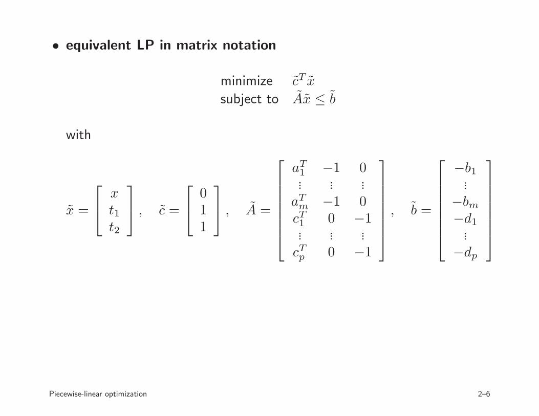
• equivalent LP in matrix notation

minimize cT x

subject to Ax ≤ b

with

x =

xt1t2

, c =

011

, A =

aT1 −1 0... ... ...aTm −1 0cT1 0 −1... ... ...cTp 0 −1

, b =

−b1...

−bm−d1...

−dp

Piecewise-linear optimization 2–6

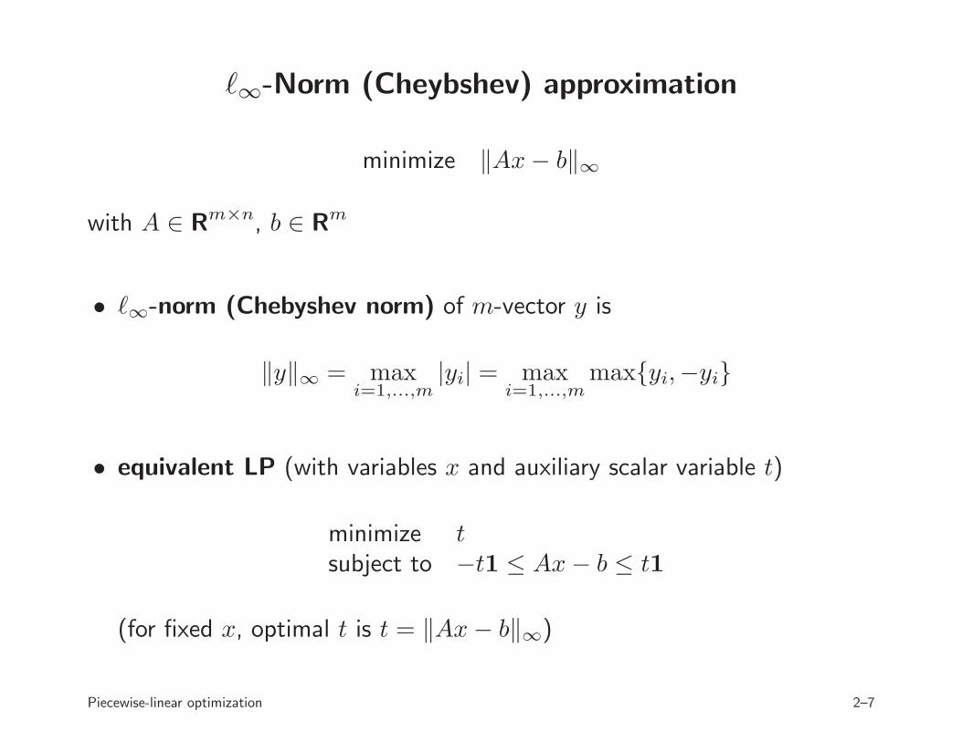
ℓ∞-Norm (Cheybshev) approximation

minimize ‖Ax− b‖∞

with A ∈ Rm×n, b ∈ Rm

• ℓ∞-norm (Chebyshev norm) of m-vector y is

‖y‖∞ = maxi=1,...,m

|yi| = maxi=1,...,m

max{yi,−yi}

• equivalent LP (with variables x and auxiliary scalar variable t)

minimize tsubject to −t1 ≤ Ax− b ≤ t1

(for fixed x, optimal t is t = ‖Ax− b‖∞)

Piecewise-linear optimization 2–7

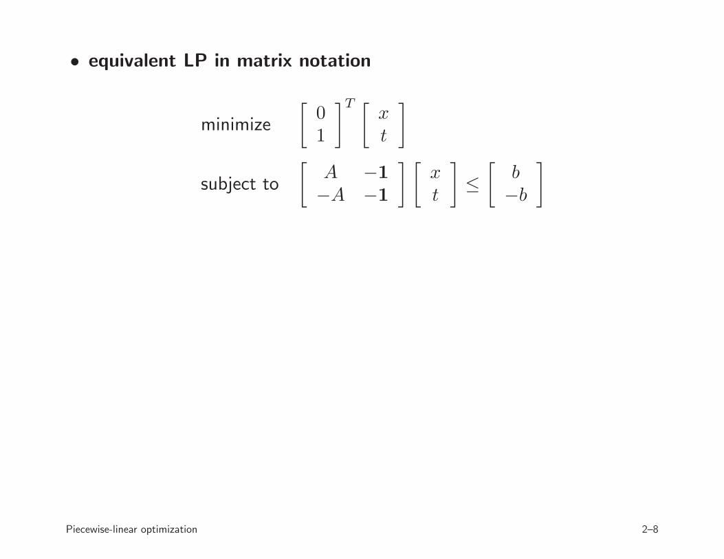
• equivalent LP in matrix notation

minimize

[

01

]T [

xt

]

subject to

[

A −1

−A −1

] [

xt

]

≤

[

b−b

]

Piecewise-linear optimization 2–8

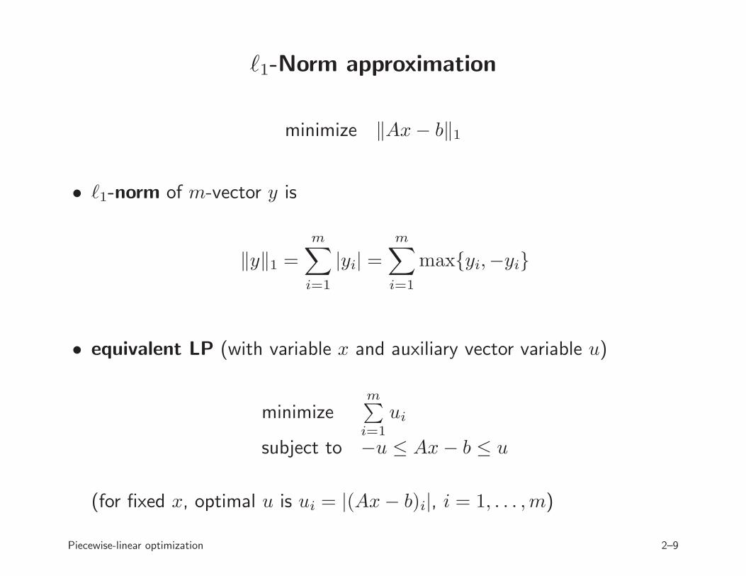
ℓ1-Norm approximation

minimize ‖Ax− b‖1

• ℓ1-norm of m-vector y is

‖y‖1 =m∑

i=1

|yi| =m∑

i=1

max{yi,−yi}

• equivalent LP (with variable x and auxiliary vector variable u)

minimizem∑

i=1

ui

subject to −u ≤ Ax− b ≤ u

(for fixed x, optimal u is ui = |(Ax− b)i|, i = 1, . . . ,m)

Piecewise-linear optimization 2–9

• equivalent LP in matrix notation

minimize

[

01

]T [

xu

]

subject to

[

A −I−A −I

] [

xu

]

≤

[

b−b

]

Piecewise-linear optimization 2–10

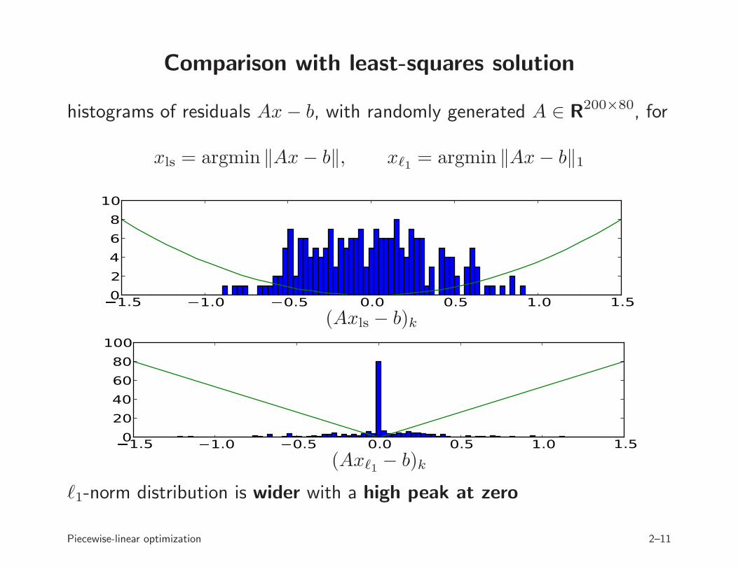
Comparison with least-squares solution

histograms of residuals Ax− b, with randomly generated A ∈ R200×80, for

xls = argmin ‖Ax− b‖, xℓ1 = argmin ‖Ax− b‖1

� 1.5 � 1.0 � 0.5 0.0 0.5 1.0 1.50246810

(Axls − b)k

� 1.5 � 1.0 � 0.5 0.0 0.5 1.0 1.5020406080100

(Axℓ1 − b)k

ℓ1-norm distribution is wider with a high peak at zero

Piecewise-linear optimization 2–11

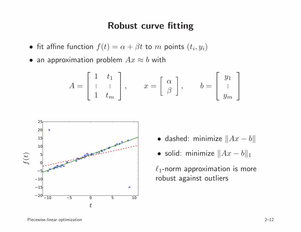
Robust curve fitting

• fit affine function f(t) = α+ βt to m points (ti, yi)

• an approximation problem Ax ≈ b with

A =

1 t1... ...1 tm

, x =

[

αβ

]

, b =

y1...ym

� 10 � 5 0 5 10� 20

� 15

� 10

� 5

0

5

10

15

20

25

t

f(t)

• dashed: minimize ‖Ax− b‖

• solid: minimize ‖Ax− b‖1

ℓ1-norm approximation is morerobust against outliers

Piecewise-linear optimization 2–12

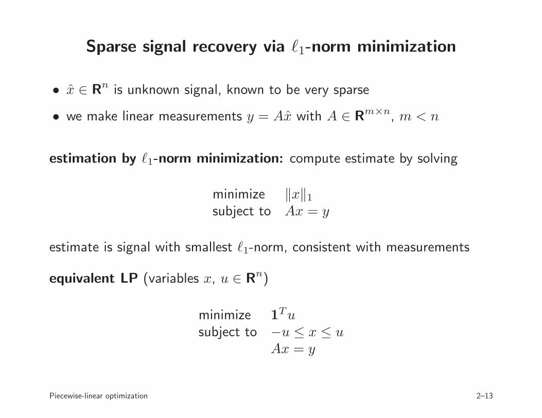
Sparse signal recovery via ℓ1-norm minimization

• x ∈ Rn is unknown signal, known to be very sparse

• we make linear measurements y = Ax with A ∈ Rm×n, m < n

estimation by ℓ1-norm minimization: compute estimate by solving

minimize ‖x‖1subject to Ax = y

estimate is signal with smallest ℓ1-norm, consistent with measurements

equivalent LP (variables x, u ∈ Rn)

minimize 1Tu

subject to −u ≤ x ≤ uAx = y

Piecewise-linear optimization 2–13

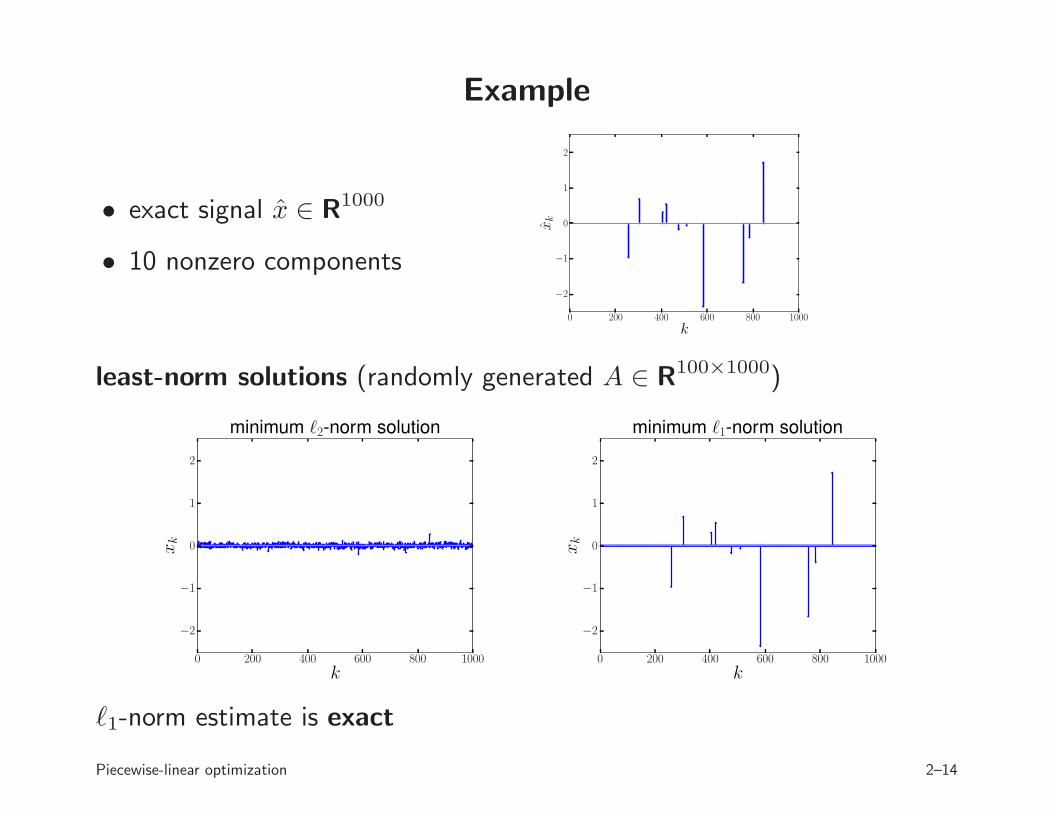
Example

• exact signal x ∈ R1000

• 10 nonzero components

0 200 400 600 800 1000

k

−2

−1

0

1

2

xk

least-norm solutions (randomly generated A ∈ R100×1000)

0 200 400 600 800 1000

k

−2

−1

0

1

2

xk

minimum ℓ2-norm solution

0 200 400 600 800 1000

k

−2

−1

0

1

2

xk

minimum ℓ1-norm solution

ℓ1-norm estimate is exact

Piecewise-linear optimization 2–14

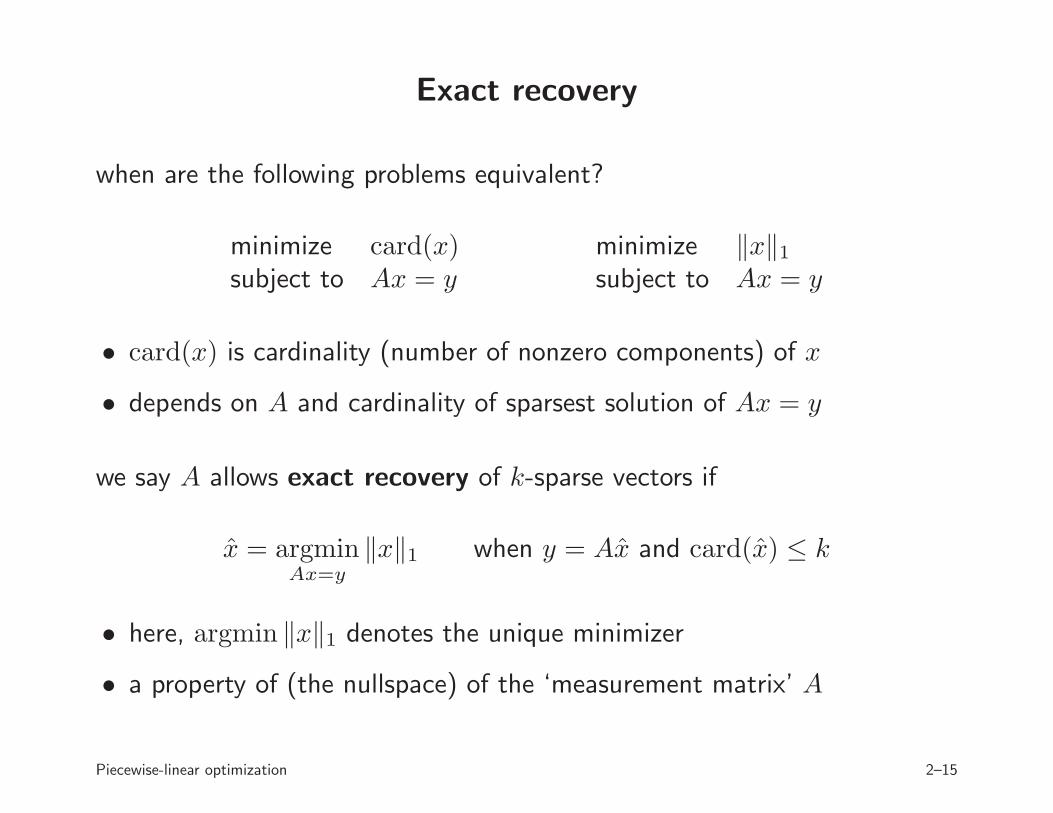
Exact recovery

when are the following problems equivalent?

minimize card(x)subject to Ax = y

minimize ‖x‖1subject to Ax = y

• card(x) is cardinality (number of nonzero components) of x

• depends on A and cardinality of sparsest solution of Ax = y

we say A allows exact recovery of k-sparse vectors if

x = argminAx=y

‖x‖1 when y = Ax and card(x) ≤ k

• here, argmin ‖x‖1 denotes the unique minimizer

• a property of (the nullspace) of the ‘measurement matrix’ A

Piecewise-linear optimization 2–15

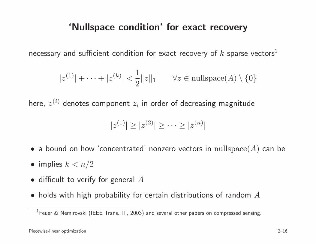
‘Nullspace condition’ for exact recovery

necessary and sufficient condition for exact recovery of k-sparse vectors1

|z(1)|+ · · ·+ |z(k)| <1

2‖z‖1 ∀z ∈ nullspace(A) \ {0}

here, z(i) denotes component zi in order of decreasing magnitude

|z(1)| ≥ |z(2)| ≥ · · · ≥ |z(n)|

• a bound on how ‘concentrated’ nonzero vectors in nullspace(A) can be

• implies k < n/2

• difficult to verify for general A

• holds with high probability for certain distributions of random A

1Feuer & Nemirovski (IEEE Trans. IT, 2003) and several other papers on compressed sensing.

Piecewise-linear optimization 2–16

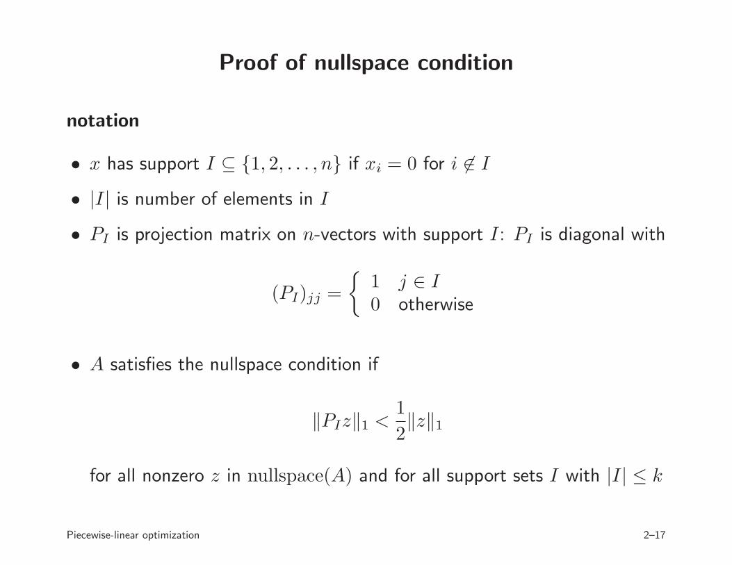
Proof of nullspace condition

notation

• x has support I ⊆ {1, 2, . . . , n} if xi = 0 for i 6∈ I

• |I| is number of elements in I

• PI is projection matrix on n-vectors with support I: PI is diagonal with

(PI)jj =

{

1 j ∈ I0 otherwise

• A satisfies the nullspace condition if

‖PIz‖1 <1

2‖z‖1

for all nonzero z in nullspace(A) and for all support sets I with |I| ≤ k

Piecewise-linear optimization 2–17

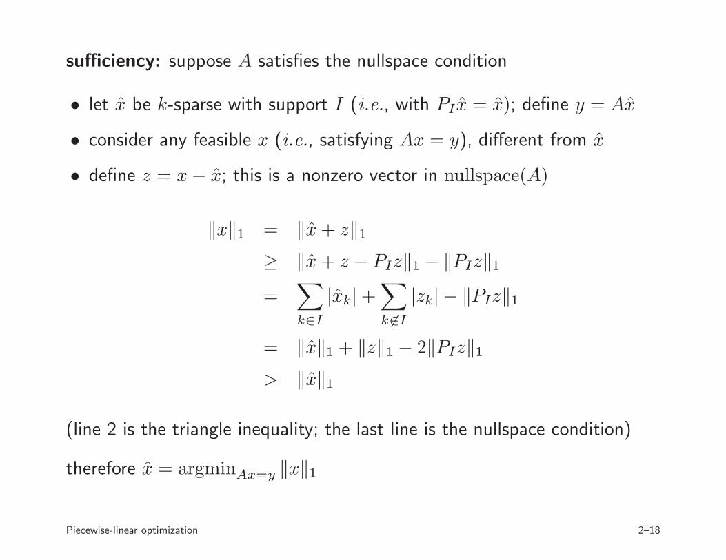
sufficiency: suppose A satisfies the nullspace condition

• let x be k-sparse with support I (i.e., with PIx = x); define y = Ax

• consider any feasible x (i.e., satisfying Ax = y), different from x

• define z = x− x; this is a nonzero vector in nullspace(A)

‖x‖1 = ‖x+ z‖1

≥ ‖x+ z − PIz‖1 − ‖PIz‖1

=∑

k∈I

|xk|+∑

k 6∈I

|zk| − ‖PIz‖1

= ‖x‖1 + ‖z‖1 − 2‖PIz‖1

> ‖x‖1

(line 2 is the triangle inequality; the last line is the nullspace condition)

therefore x = argminAx=y ‖x‖1

Piecewise-linear optimization 2–18

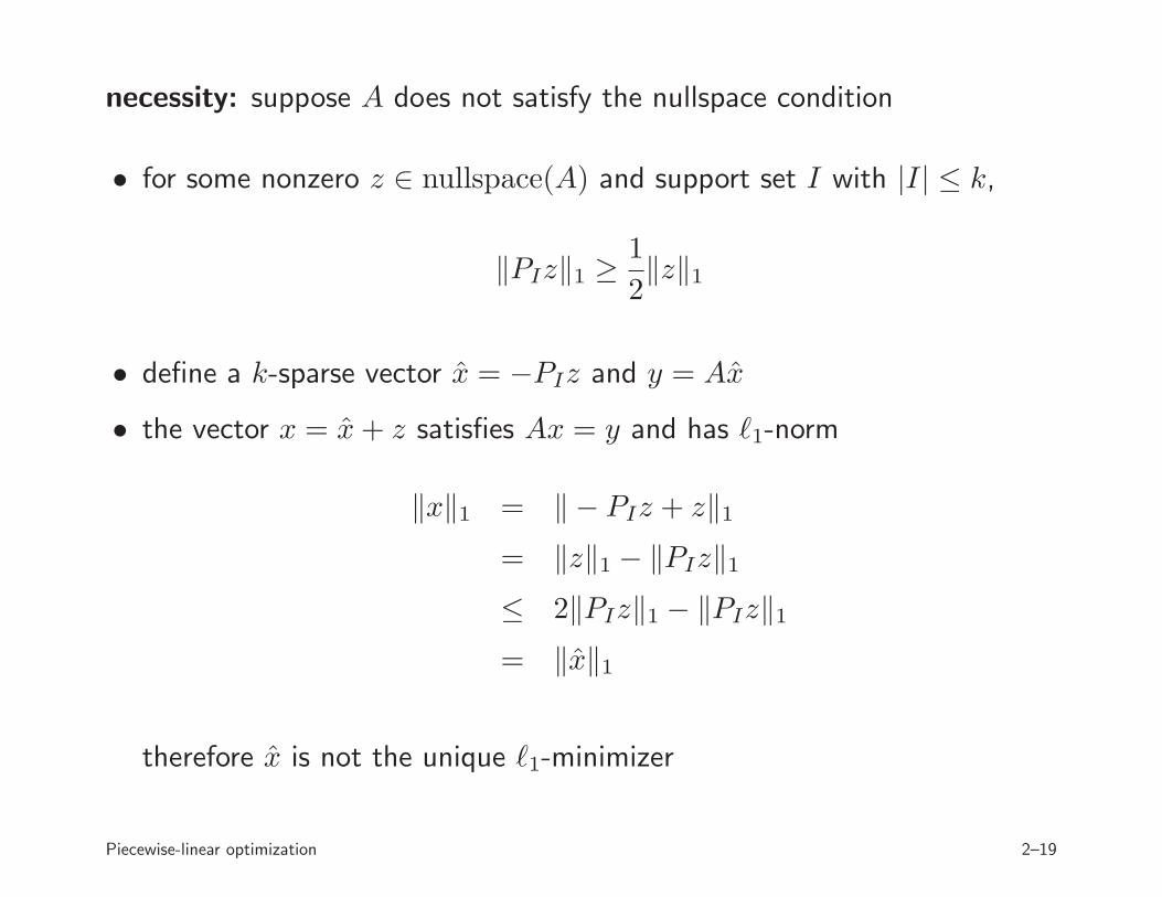
necessity: suppose A does not satisfy the nullspace condition

• for some nonzero z ∈ nullspace(A) and support set I with |I| ≤ k,

‖PIz‖1 ≥1

2‖z‖1

• define a k-sparse vector x = −PIz and y = Ax

• the vector x = x+ z satisfies Ax = y and has ℓ1-norm

‖x‖1 = ‖ − PIz + z‖1

= ‖z‖1 − ‖PIz‖1

≤ 2‖PIz‖1 − ‖PIz‖1

= ‖x‖1

therefore x is not the unique ℓ1-minimizer

Piecewise-linear optimization 2–19

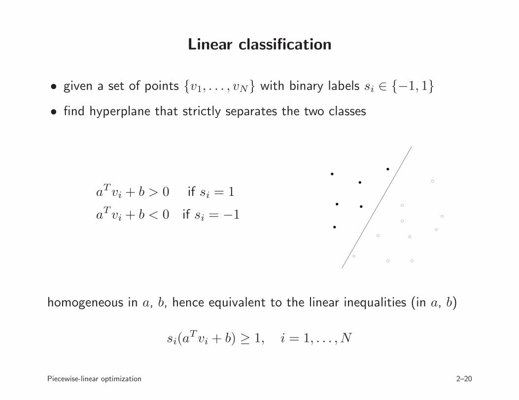
Linear classification

• given a set of points {v1, . . . , vN} with binary labels si ∈ {−1, 1}

• find hyperplane that strictly separates the two classes

aTvi + b > 0 if si = 1

aTvi + b < 0 if si = −1

homogeneous in a, b, hence equivalent to the linear inequalities (in a, b)

si(aTvi + b) ≥ 1, i = 1, . . . , N

Piecewise-linear optimization 2–20

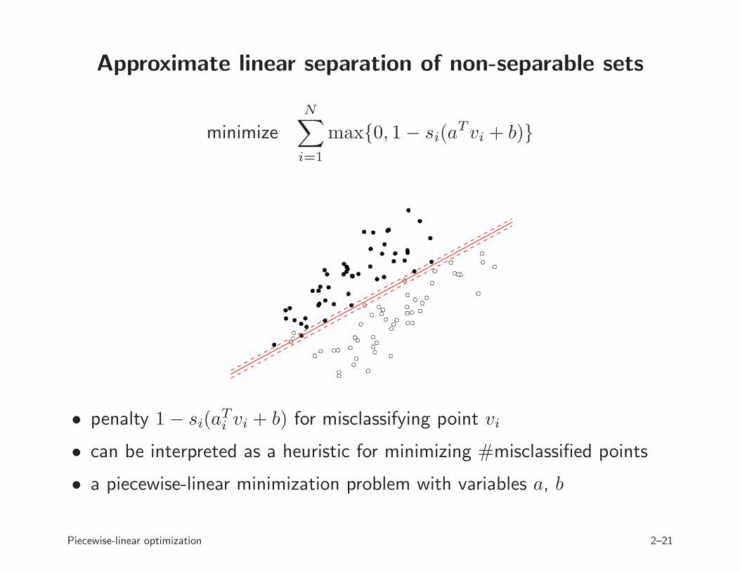
Approximate linear separation of non-separable sets

minimize

N∑

i=1

max{0, 1− si(aTvi + b)}

• penalty 1− si(aTi vi + b) for misclassifying point vi

• can be interpreted as a heuristic for minimizing #misclassified points

• a piecewise-linear minimization problem with variables a, b

Piecewise-linear optimization 2–21

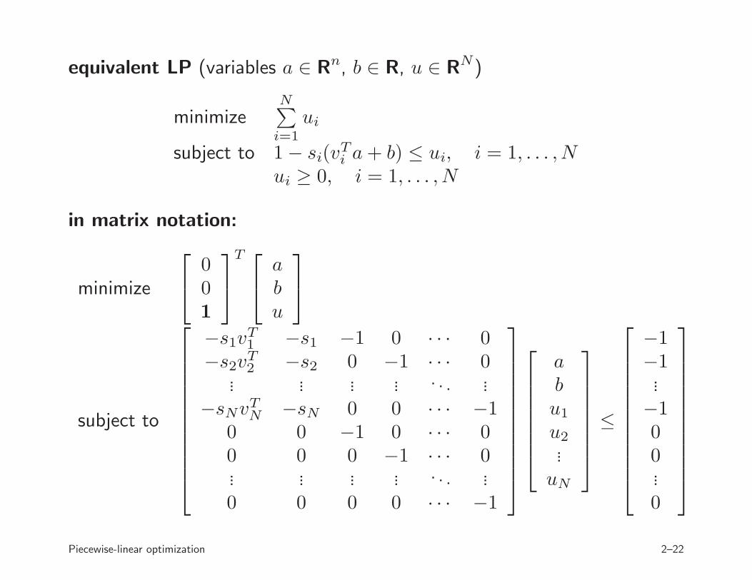
equivalent LP (variables a ∈ Rn, b ∈ R, u ∈ RN)

minimizeN∑

i=1

ui

subject to 1− si(vTi a+ b) ≤ ui, i = 1, . . . , N

ui ≥ 0, i = 1, . . . , N

in matrix notation:

minimize

001

T

abu

subject to

−s1vT1 −s1 −1 0 · · · 0

−s2vT2 −s2 0 −1 · · · 0

... ... ... ... . . . ...−sNvTN −sN 0 0 · · · −1

0 0 −1 0 · · · 00 0 0 −1 · · · 0... ... ... ... . . . ...0 0 0 0 · · · −1

abu1

u2...

uN

≤

−1−1...

−100...0

Piecewise-linear optimization 2–22

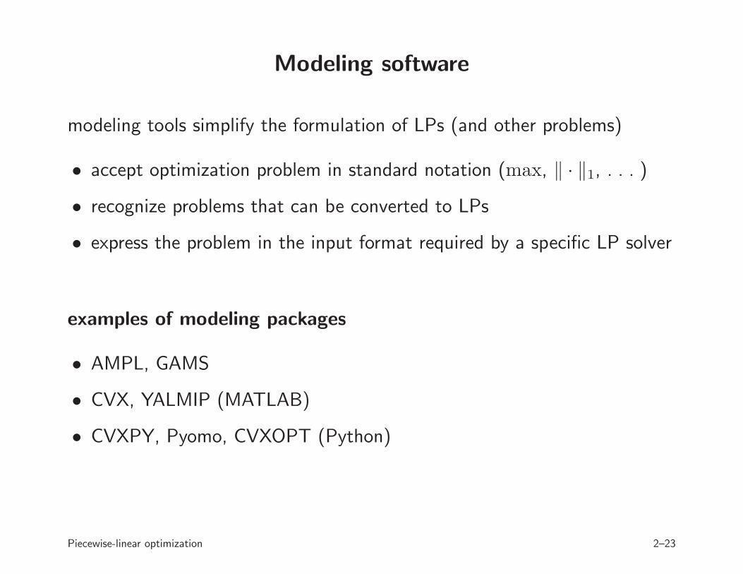
Modeling software

modeling tools simplify the formulation of LPs (and other problems)

• accept optimization problem in standard notation (max, ‖ · ‖1, . . . )

• recognize problems that can be converted to LPs

• express the problem in the input format required by a specific LP solver

examples of modeling packages

• AMPL, GAMS

• CVX, YALMIP (MATLAB)

• CVXPY, Pyomo, CVXOPT (Python)

Piecewise-linear optimization 2–23

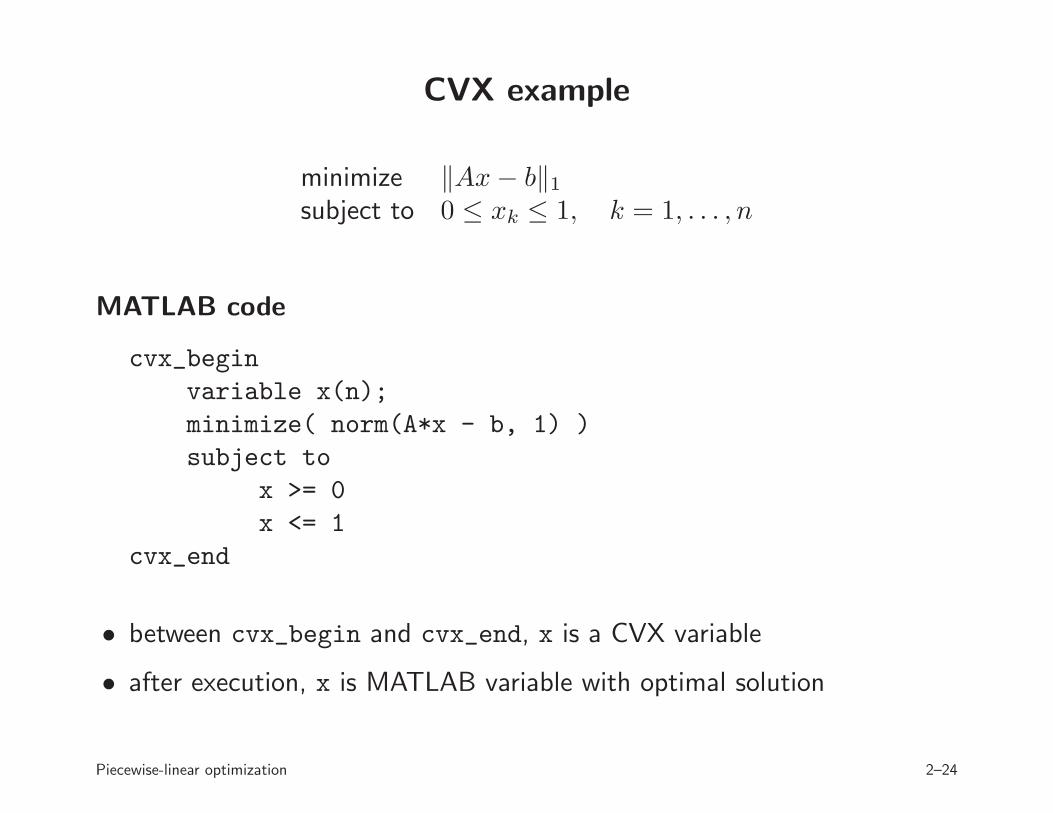
CVX example

minimize ‖Ax− b‖1subject to 0 ≤ xk ≤ 1, k = 1, . . . , n

MATLAB code

cvx_begin

variable x(n);

minimize( norm(A*x - b, 1) )

subject to

x >= 0

x <= 1

cvx_end

• between cvx_begin and cvx_end, x is a CVX variable

• after execution, x is MATLAB variable with optimal solution

Piecewise-linear optimization 2–24