Lecture 2. Linear Systems

Ivan Papusha

CDS270–2: Mathematical Methods in Control and System Engineering

April 6, 2015

1 / 31

Logistics

• hw1 due this Wed, Apr 8

• hw due every Wed

• in class, or• my mailbox on 3rd floor of Annenberg

• reading: BV Appendix A, pay attention to

• linear algebra, notation• Schur complements (also in hw1)• ≥ vs

• hw2+ will be “choose your own adventure”:

do an assigned problem

or

pick and do a problem from the catalog

2 / 31

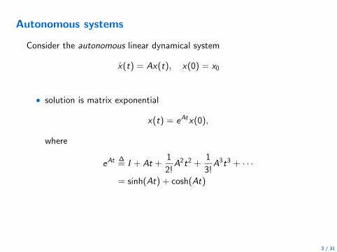
Autonomous systems

Consider the autonomous linear dynamical system

x(t) = Ax(t), x(0) = x0

• solution is matrix exponential

x(t) = eAtx(0),

where

eAt∆= I + At +

1

2!A2t2 +

1

3!A3t3 + · · ·

= sinh(At) + cosh(At)

3 / 31

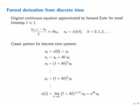
Formal derivation from discrete time

Original continuous equation approximated by forward Euler for smalltimestep δ ≪ 1

xk+1 − xk

δ≈ Axk , xk = x(kδ), k = 0, 1, 2, . . .

Classic pattern for discrete time systems:

x0 = x(0) = x0

x1 = x0 + Aδ x0

x2 = (I + Aδ)2x0

...

xk = (I + Aδ)kx0

...

x(t) = limδ→0+

(I + Aδ)⌊t/δ⌋x0 = eAtx0

4 / 31

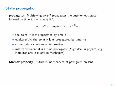
State propagation

propagator. Multiplying by eAt propagates the autonomous stateforward by time t. For v ,w ∈ Rn,

w = eAtv implies v = e−Atw .

• the point w is v propagated by time t

• equivalently: the point v is w propagated by time −t

• current state contains all information

• matrix exponential is a time propagator (huge deal in physics, e.g.,Hamiltonians in quantum mechanics)

Markov property. future is independent of past given present

5 / 31

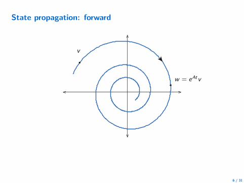
State propagation: forward

v

w = eAtv

6 / 31

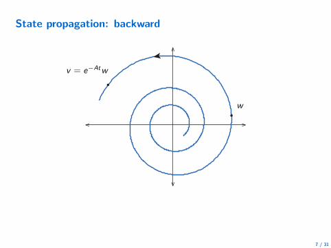
State propagation: backward

v = e−Atw

w

7 / 31

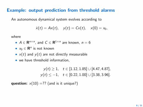
Example: output prediction from threshold alarms

An autonomous dynamical system evolves according to

x(t) = Ax(t), y(t) = Cx(t), x(0) = x0,

where

• A ∈ Rn×n, and C ∈ R1×n are known, n = 6

• x0 ∈ Rn is not known

• x(t) and y(t) are not directly measurable

• we have threshold information,

y(t) ≥ 1, t ∈ [1.12, 1.85] ∪ [4.47, 4.87],

y(t) ≤ −1, t ∈ [0.22, 1.00] ∪ [3.38, 3.96].

question: x(10) =?? (and is it unique?)

8 / 31

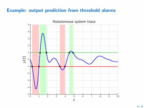
Example: output prediction from threshold alarms

0 1 2 3 4 5 6 7 8 9 10-5

-4

-3

-2

-1

0

1

2

3

4

5

t

y(t)Autonomous system trace

9 / 31

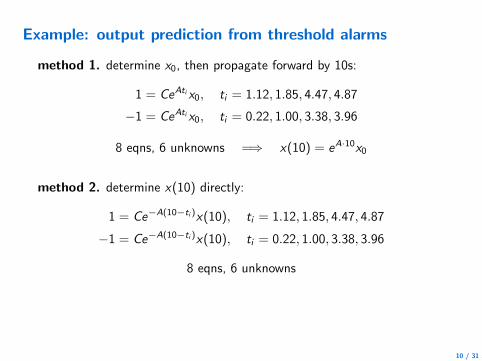
Example: output prediction from threshold alarms

method 1. determine x0, then propagate forward by 10s:

1 = CeAti x0, ti = 1.12, 1.85, 4.47, 4.87

−1 = CeAti x0, ti = 0.22, 1.00, 3.38, 3.96

8 eqns, 6 unknowns =⇒ x(10) = eA·10x0

method 2. determine x(10) directly:

1 = Ce−A(10−ti )x(10), ti = 1.12, 1.85, 4.47, 4.87

−1 = Ce−A(10−ti )x(10), ti = 0.22, 1.00, 3.38, 3.96

8 eqns, 6 unknowns

10 / 31

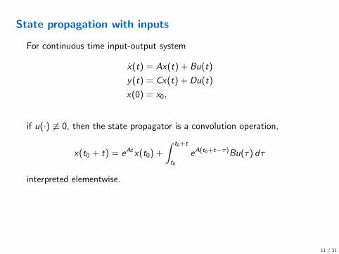
State propagation with inputs

For continuous time input-output system

x(t) = Ax(t) + Bu(t)

y(t) = Cx(t) + Du(t)

x(0) = x0,

if u(·) 6≡ 0, then the state propagator is a convolution operation,

x(t0 + t) = eAtx(t0) +

∫ t0+t

t0

eA(t0+t−τ)Bu(τ) dτ

interpreted elementwise.

11 / 31

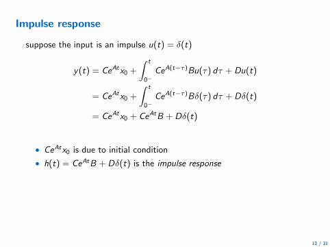
Impulse response

suppose the input is an impulse u(t) = δ(t)

y(t) = CeAtx0 +

∫ t

0−CeA(t−τ)Bu(τ) dτ + Du(t)

= CeAtx0 +

∫ t

0−CeA(t−τ)Bδ(τ) dτ + Dδ(t)

= CeAtx0 + CeAtB + Dδ(t)

• CeAtx0 is due to initial condition

• h(t) = CeAtB + Dδ(t) is the impulse response

12 / 31

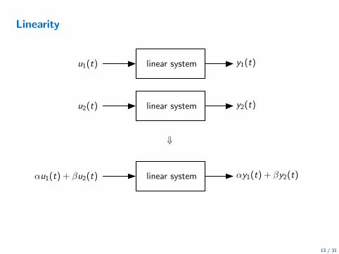
Linearity

linear systemu1(t) y1(t)

linear systemu2(t) y2(t)

⇓

linear systemαu1(t) + βu2(t) αy1(t) + βy2(t)

13 / 31

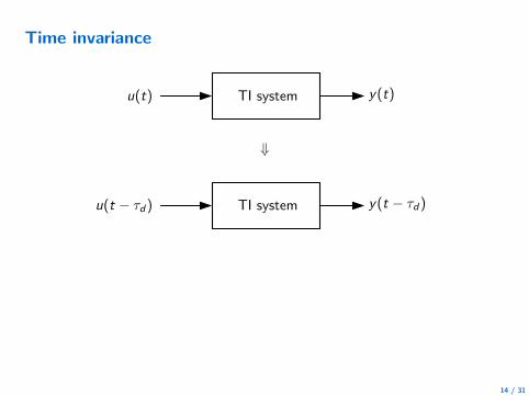
Time invariance

TI systemu(t) y(t)

⇓

TI systemu(t − τd) y(t − τd)

14 / 31

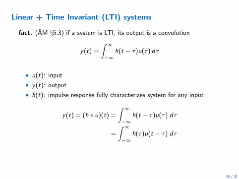
Linear + Time Invariant (LTI) systems

fact. (AM §5.3) if a system is LTI, its output is a convolution

y(t) =

∫ ∞

−∞

h(t − τ)u(τ) dτ

• u(t): input

• y(t): output

• h(t): impulse response fully characterizes system for any input

y(t) = (h ∗ u)(t) =∫ ∞

−∞

h(t − τ)u(τ) dτ

=

∫ ∞

−∞

h(τ)u(t − τ) dτ

15 / 31

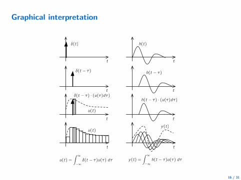
Graphical interpretation

δ(t) h(t)

δ(t − τ)h(t − τ)

t

t

t

t

t

t

δ(t − τ) · (u(τ)dτ)h(t − τ) · (u(τ)dτ)

t t

u(t) =

∫∞

−∞

δ(t − τ)u(τ) dτ y(t) =

∫∞

−∞

h(t − τ)u(τ) dτ

u(t)

u(t)y(t)

16 / 31

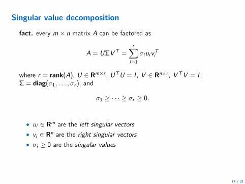
Singular value decomposition

fact. every m × n matrix A can be factored as

A = UΣV T =

r∑

i=1

σiuivTi

where r = rank(A), U ∈ Rm×r , UTU = I , V ∈ Rn×r , V TV = I ,Σ = diag(σ1, . . . , σr ), and

σ1 ≥ · · · ≥ σr ≥ 0.

• ui ∈ Rm are the left singular vectors

• vi ∈ Rn are the right singular vectors

• σi ≥ 0 are the singular values

17 / 31

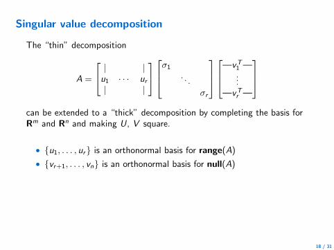
Singular value decomposition

The “thin” decomposition

A =

| |u1 · · · ur| |

σ1

. . .

σr

—vT1 —...

—vTr —

can be extended to a “thick” decomposition by completing the basis forRm and Rn and making U, V square.

• u1, . . . , ur is an orthonormal basis for range(A)

• vr+1, . . . , vn is an orthonormal basis for null(A)

18 / 31

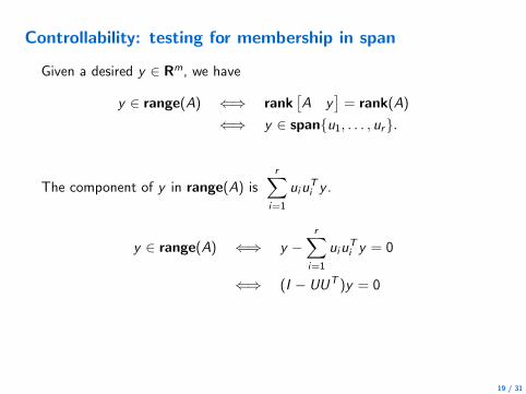
Controllability: testing for membership in span

Given a desired y ∈ Rm, we have

y ∈ range(A) ⇐⇒ rank[A y

]= rank(A)

⇐⇒ y ∈ spanu1, . . . , ur.

The component of y in range(A) is

r∑

i=1

uiuTi y .

y ∈ range(A) ⇐⇒ y −r∑

i=1

uiuTi y = 0

⇐⇒ (I − UUT )y = 0

19 / 31

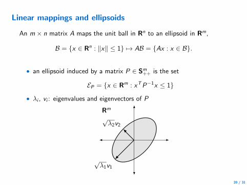
Linear mappings and ellipsoids

An m × n matrix A maps the unit ball in Rn to an ellipsoid in Rm,

B = x ∈ Rn : ‖x‖ ≤ 1 7→ AB = Ax : x ∈ B.

• an ellipsoid induced by a matrix P ∈ Sm++ is the set

EP = x ∈ Rm : xTP−1x ≤ 1

• λi , vi : eigenvalues and eigenvectors of P

√λ1v1

√λ2v2

Rm

20 / 31

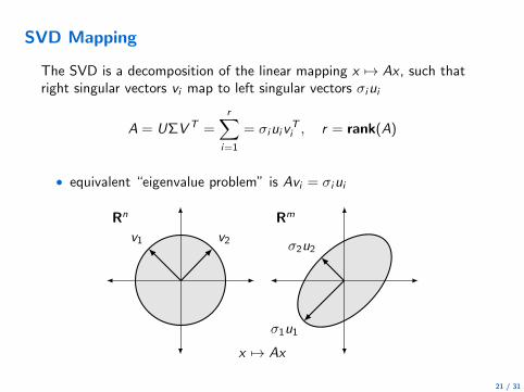
SVD Mapping

The SVD is a decomposition of the linear mapping x 7→ Ax , such thatright singular vectors vi map to left singular vectors σiui

A = UΣV T =

r∑

i=1

= σiuivTi , r = rank(A)

• equivalent “eigenvalue problem” is Avi = σiui

v1 v2

σ1u1

σ2u2

Rn Rm

x 7→ Ax

21 / 31

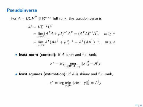
Pseudoinverse

For A = UΣV T ∈ Rm×n full rank, the pseudoinverse is

A† = VΣ−1UT

= limµ→0

(ATA+ µI )−1AT = (ATA)−1AT , m ≥ n

= limµ→0

AT (AAT + µI )−1 = AT (AAT )−1, m ≤ n

• least norm (control): if A is fat and full rank,

x⋆ = arg minx∈Rn,Ax=y

‖x‖22 = A†y

• least squares (estimation): if A is skinny and full rank,

x⋆ = arg minx∈Rn

‖Ax − y‖22 = A†y

22 / 31

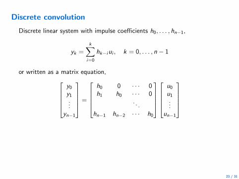
Discrete convolution

Discrete linear system with impulse coefficients h0, . . . , hn−1,

yk =

k∑

i=0

hk−iui , k = 0, . . . , n − 1

or written as a matrix equation,

y0y1...

yn−1

=

h0 0 · · · 0h1 h0 · · · 0

. . .

hn−1 hn−2 · · · h0

u0u1...

un−1

23 / 31

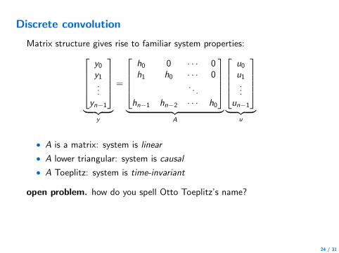
Discrete convolution

Matrix structure gives rise to familiar system properties:

y0y1...

yn−1

︸ ︷︷ ︸

y

=

h0 0 · · · 0h1 h0 · · · 0

. . .

hn−1 hn−2 · · · h0

︸ ︷︷ ︸

A

u0u1...

un−1

︸ ︷︷ ︸

u

• A is a matrix: system is linear

• A lower triangular: system is causal

• A Toeplitz: system is time-invariant

open problem. how do you spell Otto Toeplitz’s name?

24 / 31

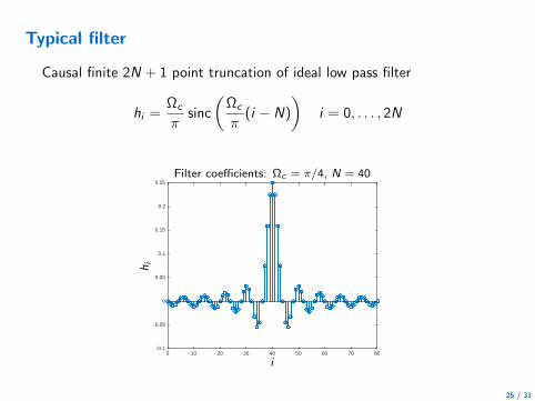
Typical filter

Causal finite 2N + 1 point truncation of ideal low pass filter

hi =Ωc

πsinc

(Ωc

π(i − N)

)

i = 0, . . . , 2N

0 10 20 30 40 50 60 70 80-0.1

-0.05

0

0.05

0.1

0.15

0.2

0.25

i

hi

Filter coefficients: Ωc = π/4, N = 40

25 / 31

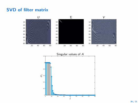
SVD of filter matrix

20 40 60 80

10

20

30

40

50

60

70

8020 40 60 80

10

20

30

40

50

60

70

8020 40 60 80

10

20

30

40

50

60

70

80

U Σ V

0 10 20 30 40 50 60 70 800

0.2

0.4

0.6

0.8

1

1.2

i

σi

Singular values of A

26 / 31

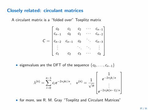
Closely related: circulant matrices

A circulant matrix is a “folded over” Toeplitz matrix

C =

c0 c1 c2 · · · cn−1

cn−1 c0 c1 · · · cn−2

cn−2 cn−1 c0. . . cn−3

.... . .

. . ....

c1 c2 c3 · · · c0

• eigenvalues are the DFT of the sequence c0, . . . , cn−1

λ(k) =

n−1∑

i=0

cie−2πjki/n, v (k) =

1√n

1e−2πjk/n

...e−2πjk(n−1)/n

• for more, see R. M. Gray “Toeplitz and Circulant Matrices”

27 / 31

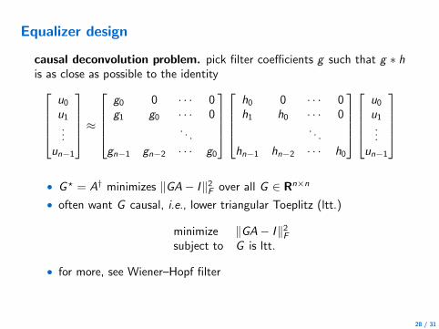
Equalizer design

causal deconvolution problem. pick filter coefficients g such that g ∗ his as close as possible to the identity

u0u1...

un−1

≈

g0 0 · · · 0g1 g0 · · · 0

. . .

gn−1 gn−2 · · · g0

h0 0 · · · 0h1 h0 · · · 0

. . .

hn−1 hn−2 · · · h0

u0u1...

un−1

• G⋆ = A† minimizes ‖GA− I‖2F over all G ∈ Rn×n

• often want G causal, i.e., lower triangular Toeplitz (ltt.)

minimize ‖GA− I‖2Fsubject to G is ltt.

• for more, see Wiener–Hopf filter

28 / 31

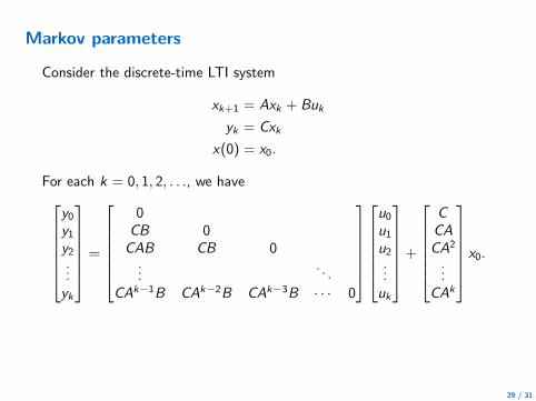
Markov parameters

Consider the discrete-time LTI system

xk+1 = Axk + Buk

yk = Cxk

x(0) = x0.

For each k = 0, 1, 2, . . ., we have

y0y1y2...yk

=

0CB 0CAB CB 0...

. . .

CAk−1B CAk−2B CAk−3B · · · 0

u0u1u2...uk

+

C

CA

CA2

...CAk

x0.

29 / 31

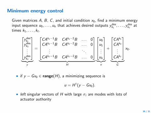
Minimum energy control

Given matrices A, B , C , and initial condition x0, find a minimum energyinput sequence u0, . . . , uk that achieves desired outputs ydes

k1, . . . , ydes

kℓat

times k1, . . . , kℓ.

ydesk1

ydesk2...

ydeskℓ

︸ ︷︷ ︸

y

=

CAk1−1B CAk1−2B . . . 0CAk2−1B CAk2−2B . . . 0

.... . .

CAkℓ−1B CAkℓ−2B . . . 0

︸ ︷︷ ︸

H

u0u1...uk

︸ ︷︷ ︸

u

+

CAk1

CAk2

...CAkℓ

︸ ︷︷ ︸

G

x0.

• if y − Gx0 ∈ range(H), a minimizing sequence is

u = H†(y − Gx0).

• left singular vectors of H with large σi are modes with lots ofactuator authority

30 / 31

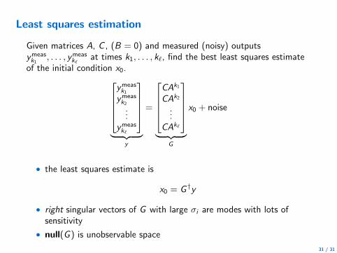
Least squares estimation

Given matrices A, C , (B = 0) and measured (noisy) outputsymeask1

, . . . , ymeaskℓ

at times k1, . . . , kℓ, find the best least squares estimateof the initial condition x0.

ymeask1

ymeask2...

ymeaskℓ

︸ ︷︷ ︸

y

=

CAk1

CAk2

...CAkℓ

︸ ︷︷ ︸

G

x0 + noise

• the least squares estimate is

x0 = G †y

• right singular vectors of G with large σi are modes with lots ofsensitivity

• null(G ) is unobservable space

31 / 31