Lecture 18, p 1

Lecture 18:Orbitals and Spin

1

0

1

θ

y

z

x

Lecture 18, p 2

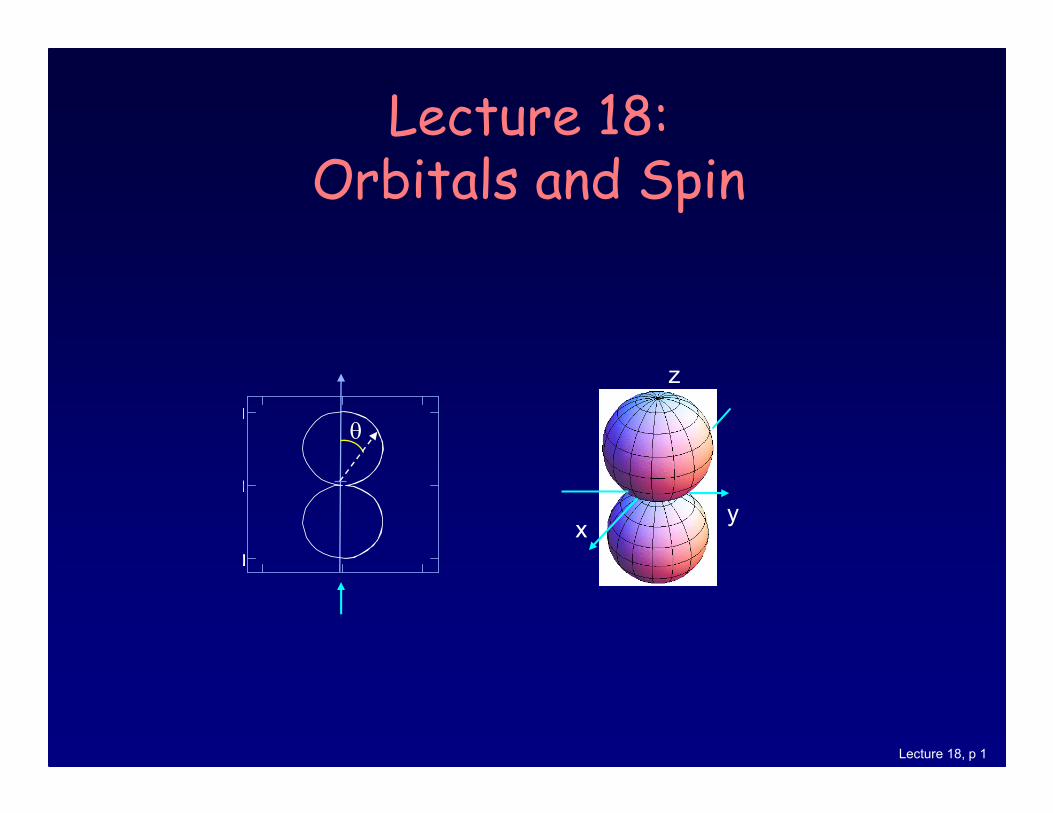
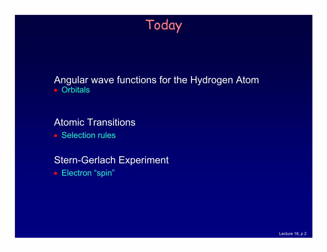
Today

Angular wave functions for the Hydrogen Atom • Orbitals

Atomic Transitions

• Selection rules

Stern-Gerlach Experiment

• Electron “spin”

Lecture 18, p 3

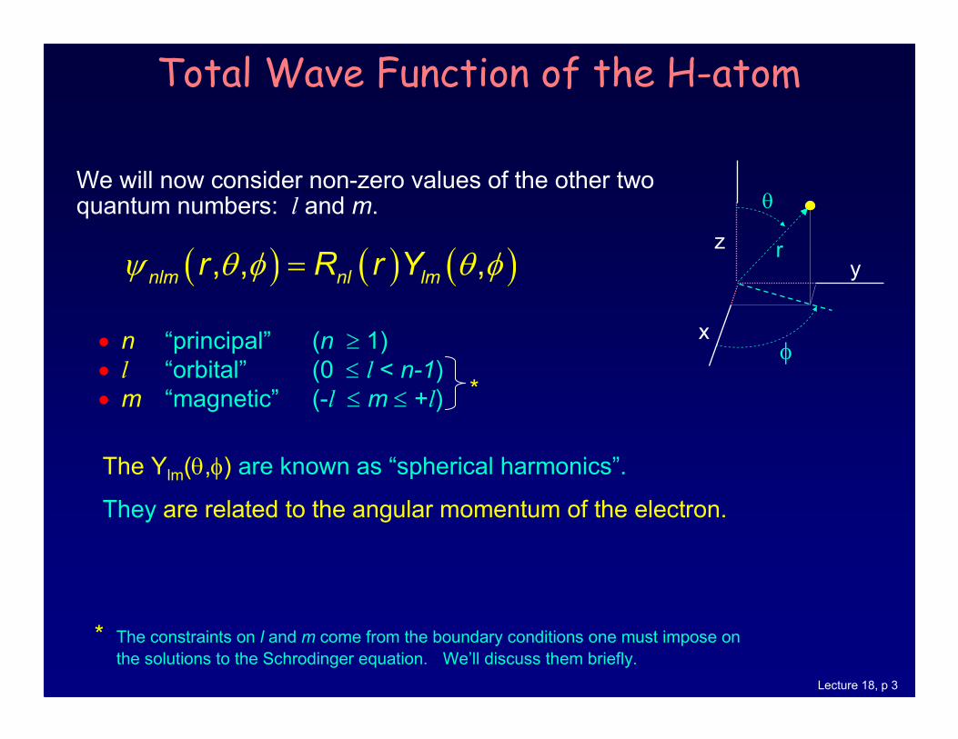
The Ylm(θ,φ) are known as “spherical harmonics”.

They are related to the angular momentum of the electron.

Total Wave Function of the H-atom

We will now consider non-zero values of the other two quantum numbers: l and m.

• n “principal” (n ≥ 1)

• l “orbital” (0 ≤ l < n-1)

• m “magnetic” (-l ≤ m ≤ +l)

( ) ( ) ( ), , ,nlm nl lmr R r Yψ θ φ θ φ=

x

y

z r

θ

φ

* The constraints on l and m come from the boundary conditions one must impose on

the solutions to the Schrodinger equation. We’ll discuss them briefly.

*

Lecture 18, p 4

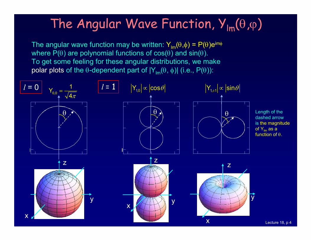
The Angular Wave Function, Ylm(θ,ϕ)

The angular wave function may be written: Ylm(θ,φ) = P(θ)eimφ

where P(θ) are polynomial functions of cos(θ) and sin(θ).

To get some feeling for these angular distributions, we make

polar plots of the θ-dependent part of |Ylm(θ, φ)| (i.e., P(θ)):

1

θ

l = 00,0

1Y

4π=

z

x

y

l = 1

1

0

1

θ

1,0Y cosθ∝

y

z

x

z

x

y

1, 1Y sinθ± ∝

θ Length of the

dashed arrow

is the magnitude

of Ylm as a

function of θ.

Lecture 18, p 5

2

Parametric Curve

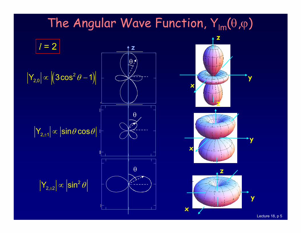
The Angular Wave Function, Ylm(θ,ϕ)

l = 2

1

0

1

Parametric Curve

1

z

( )2

2,0Y 3cos 1θ∝ −

2, 1Y sin cosθ θ± ∝

2

2, 2Y sin θ± ∝

θ

θ

z

xy

z

xy

z

-

+

y

x

θ

Lecture 18, p 6

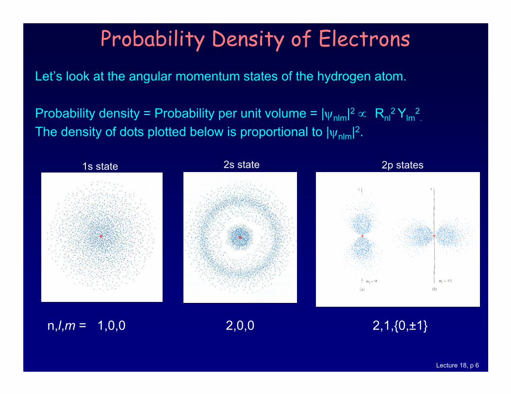
Probability Density of Electrons

Let’s look at the angular momentum states of the hydrogen atom.

Probability density = Probability per unit volume = |ψnlm|2 ∝ Rnl2 Ylm

2.

The density of dots plotted below is proportional to |ψnlm|2.

1s state 2s state 2p states

n,l,m = 1,0,0 2,0,0 2,1,{0,±1}

Lecture 18, p 7

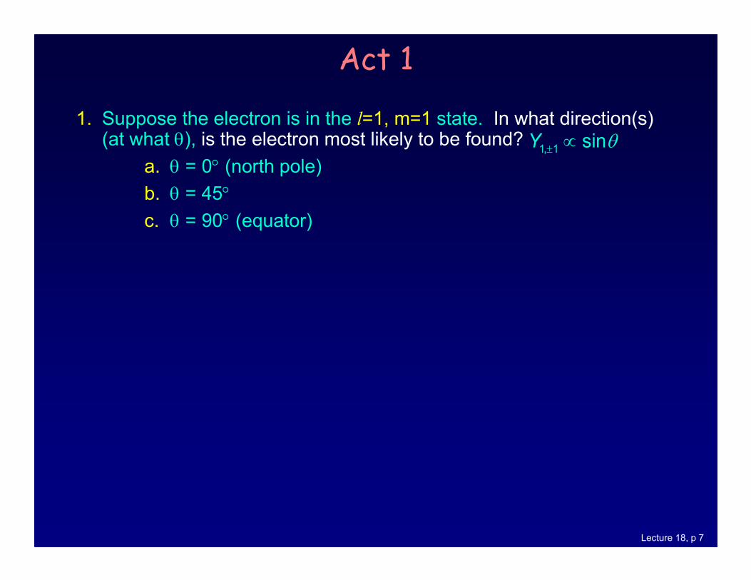
1. Suppose the electron is in the l=1, m=1 state. In what direction(s) (at what θ), is the electron most likely to be found?

a. θ = 0° (north pole)

b. θ = 45°

c. θ = 90° (equator)

Act 1

1, 1 sinY θ± ∝

Lecture 18, p 8

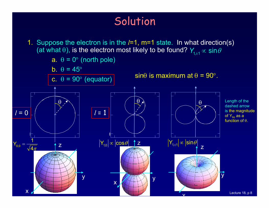
1. Suppose the electron is in the l=1, m=1 state. In what direction(s) (at what θ), is the electron most likely to be found?

a. θ = 0° (north pole)

b. θ = 45°

c. θ = 90° (equator)

Solution

sinθ is maximum at θ = 90°.

1, 1 sinY θ± ∝

1

θ

l = 0

0,0

1Y

4π= z

x

y

l = 1

1

0

1

θ

1,0Y cosθ∝

y

z

x

z

x

y

1, 1Y sinθ± ∝

θ Length of the

dashed arrow

is the magnitude

of Ylm as a

function of θ.

Lecture 18, p 9

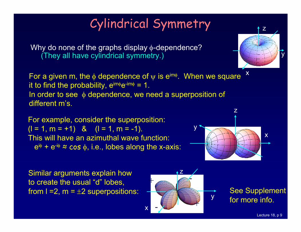
Cylindrical Symmetry

Why do none of the graphs display φ-dependence?(They all have cylindrical symmetry.)

For a given m, the φ dependence of ψ is eimφ. When we square

it to find the probability, eimφe-imφ = 1.

In order to see φ dependence, we need a superposition of

different m’s.

y

z

x

Similar arguments explain how

to create the usual “d” lobes,

from l =2, m = ±2 superpositions:

z

-

+ -

+y

x

For example, consider the superposition:

(l = 1, m = +1) & (l = 1, m = -1).

This will have an azimuthal wave function:

eiφ + e-iφ ≈ cos φ, i.e., lobes along the x-axis:

See Supplement

for more info.

z

x

y

Lecture 18, p 10

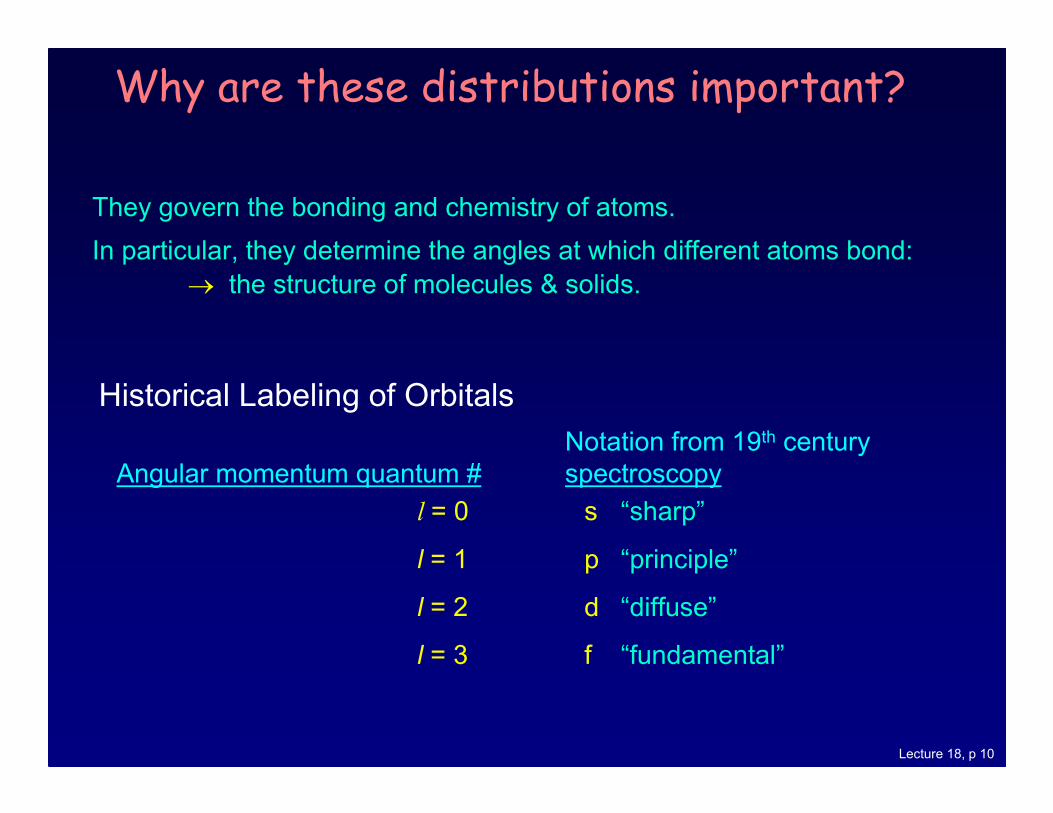
They govern the bonding and chemistry of atoms.

In particular, they determine the angles at which different atoms bond:

→ the structure of molecules & solids.

Why are these distributions important?

Historical Labeling of Orbitals

Notation from 19th century

Angular momentum quantum # spectroscopy

l = 0 s “sharp”

l = 1 p “principle”

l = 2 d “diffuse”

l = 3 f “fundamental”

Lecture 18, p 11

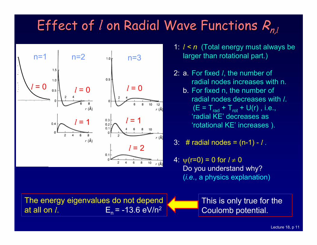
Effect of Effect of l on Radial Wave Functions on Radial Wave Functions RRn,n,ll

1: l < n (Total energy must always be

larger than rotational part.)

2: a. For fixed l, the number of

radial nodes increases with n.

b. For fixed n, the number of

radial nodes decreases with l.

(E = Trad + Trot + U(r) , i.e.,

‘radial KE’ decreases as

‘rotational KE’ increases ).

3: # radial nodes = (n-1) - l .

4: ψ(r=0) = 0 for l ≠ 0

Do you understand why?

(i.e., a physics explanation)

The energy eigenvalues do not depend

at all on l. En = -13.6 eV/n2

This is only true for the

Coulomb potential.

l = 2

l = 1

l = 0

l = 1

l = 0

n=2 n=3

l = 0

n=1

Lecture 18, p 12

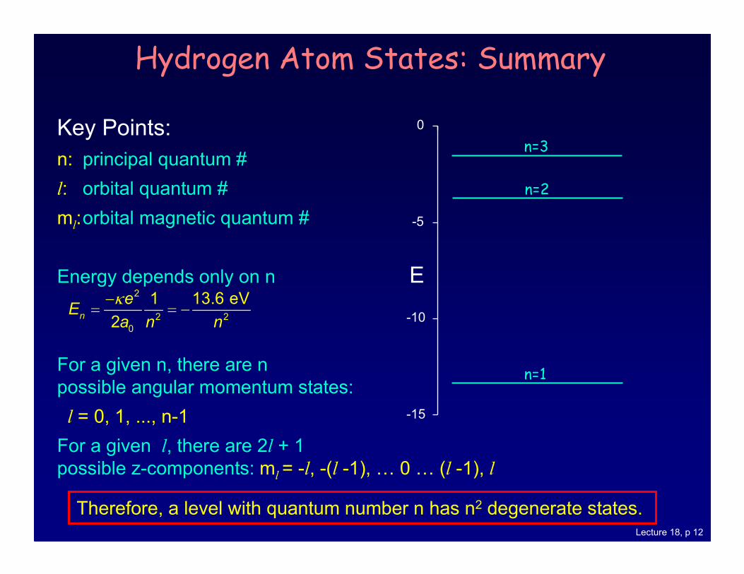
Hydrogen Atom States: Summary

Key Points:

n: principal quantum #

l: orbital quantum #

ml:orbital magnetic quantum #

Energy depends only on n

For a given n, there are n

possible angular momentum states:

l = 0, 1, ..., n-1

For a given l, there are 2l + 1

possible z-components: ml = -l, -(l -1), O 0 O (l -1), l

Therefore, a level with quantum number n has n2 degenerate states.

2

2 2

0

1 13.6 eV

2n

eE

a n n

κ−= = −

n=1

n=3

n=2

E

-15

-10

-5

0

Lecture 18, p 13

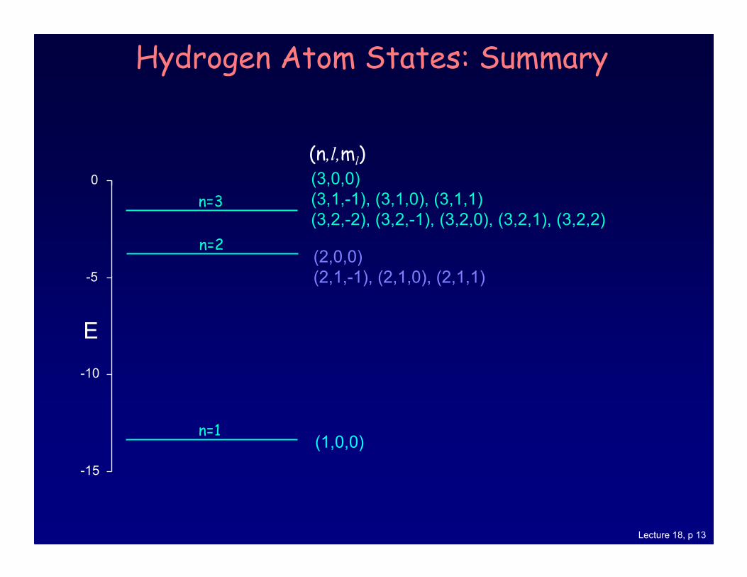
Hydrogen Atom States: Summary

(1,0,0)

(2,0,0)

(2,1,-1), (2,1,0), (2,1,1)

(3,0,0)

(3,1,-1), (3,1,0), (3,1,1)

(3,2,-2), (3,2,-1), (3,2,0), (3,2,1), (3,2,2)

(n,l,ml)

n=1

n=3

n=2

E

-15

-10

-5

0

Lecture 18, p 14

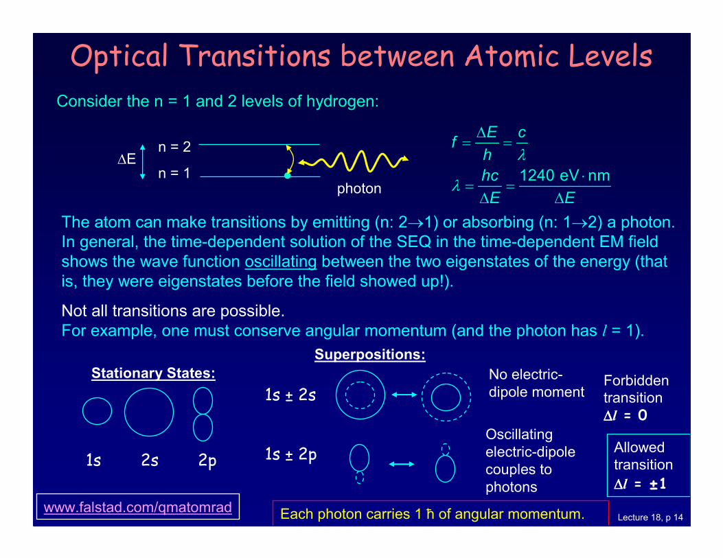
Optical Transitions between Atomic Levels

Consider the n = 1 and 2 levels of hydrogen:

The atom can make transitions by emitting (n: 2→1) or absorbing (n: 1→2) a photon.

In general, the time-dependent solution of the SEQ in the time-dependent EM field

shows the wave function oscillating between the two eigenstates of the energy (that

is, they were eigenstates before the field showed up!).

Not all transitions are possible.

For example, one must conserve angular momentum (and the photon has l = 1).

1240 eV nm

E cf

h

hc

E E

λ

λ

∆= =

⋅= =

∆ ∆

n = 2

n = 1∆E

photon

Each photon carries 1 ћ of angular momentum.

1s 2s 2p

Stationary States:

Superpositions:

1s ± 2s

1s ± 2pOscillating

electric-dipole

couples to

photons

No electric-

dipole momentForbidden

transition

∆∆∆∆l = 0

Allowed

transition

∆∆∆∆l = ±1

www.falstad.com/qmatomrad

Lecture 18, p 15

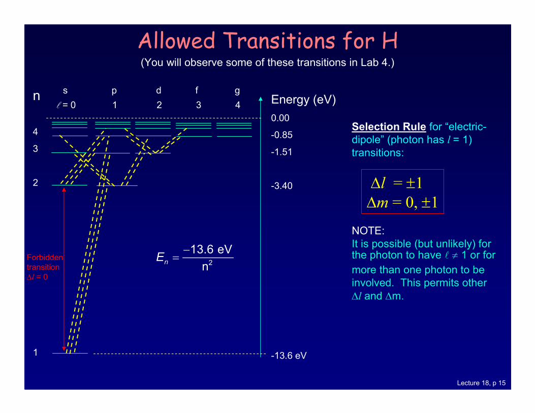
Allowed Transitions for H

Selection Rule for “electric-

dipole” (photon has l = 1)

transitions:

NOTE:

It is possible (but unlikely) for the photon to have ℓ ≠ 1 or for

more than one photon to be

involved. This permits other

∆l and ∆m.

(You will observe some of these transitions in Lab 4.)

∆l = ±1∆m = 0, ±1

Energy (eV)

0.00

-0.85

-1.51

-3.40

-13.6 eV

n

4

3

2

1

ℓ = 0 1 2 3 4

s p d f g

2

13.6 eV

nnE

−=Forbidden

transition

∆l = 0

Lecture 18, p 16

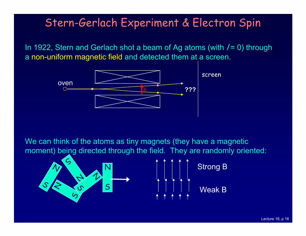
In 1922, Stern and Gerlach shot a beam of Ag atoms (with l = 0) through

a non-uniform magnetic field and detected them at a screen.

We can think of the atoms as tiny magnets (they have a magnetic

moment) being directed through the field. They are randomly oriented:

Stern-Gerlach Experiment & Electron Spin

screen

???

Strong B

Weak B

N

SN

S

N

S

N

S

N

S

B

oven

Lecture 18, p 17

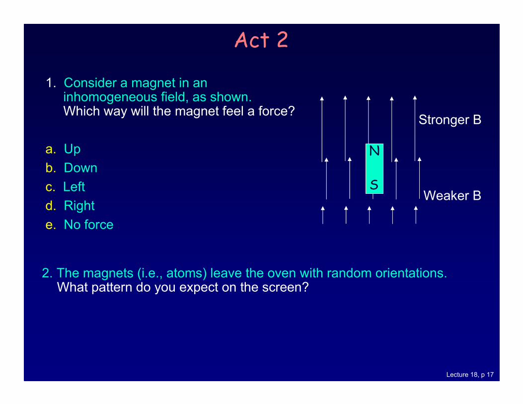
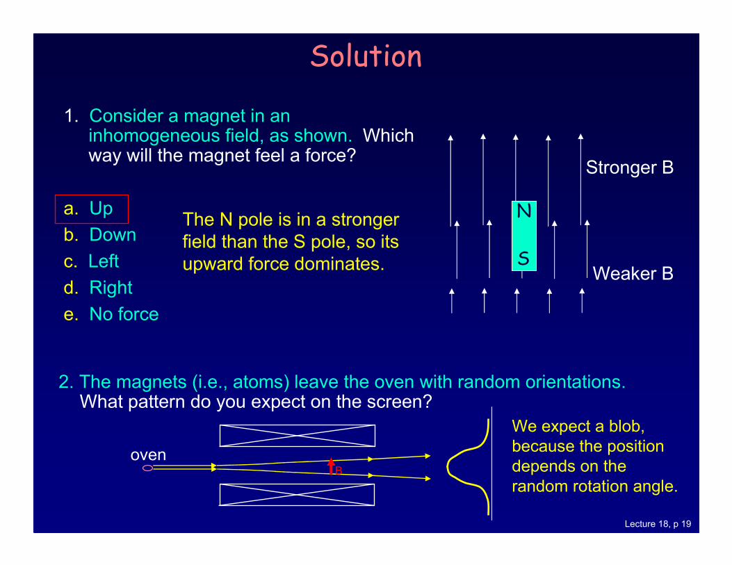
2. The magnets (i.e., atoms) leave the oven with random orientations.What pattern do you expect on the screen?

Act 2

1. Consider a magnet in an inhomogeneous field, as shown. Which way will the magnet feel a force?

a. Up

b. Down

c. Left

d. Right

e. No force

Stronger B

Weaker B

N

S

Lecture 18, p 18

2. The magnets (i.e., atoms) leave the oven with random orientations.What pattern do you expect on the screen?

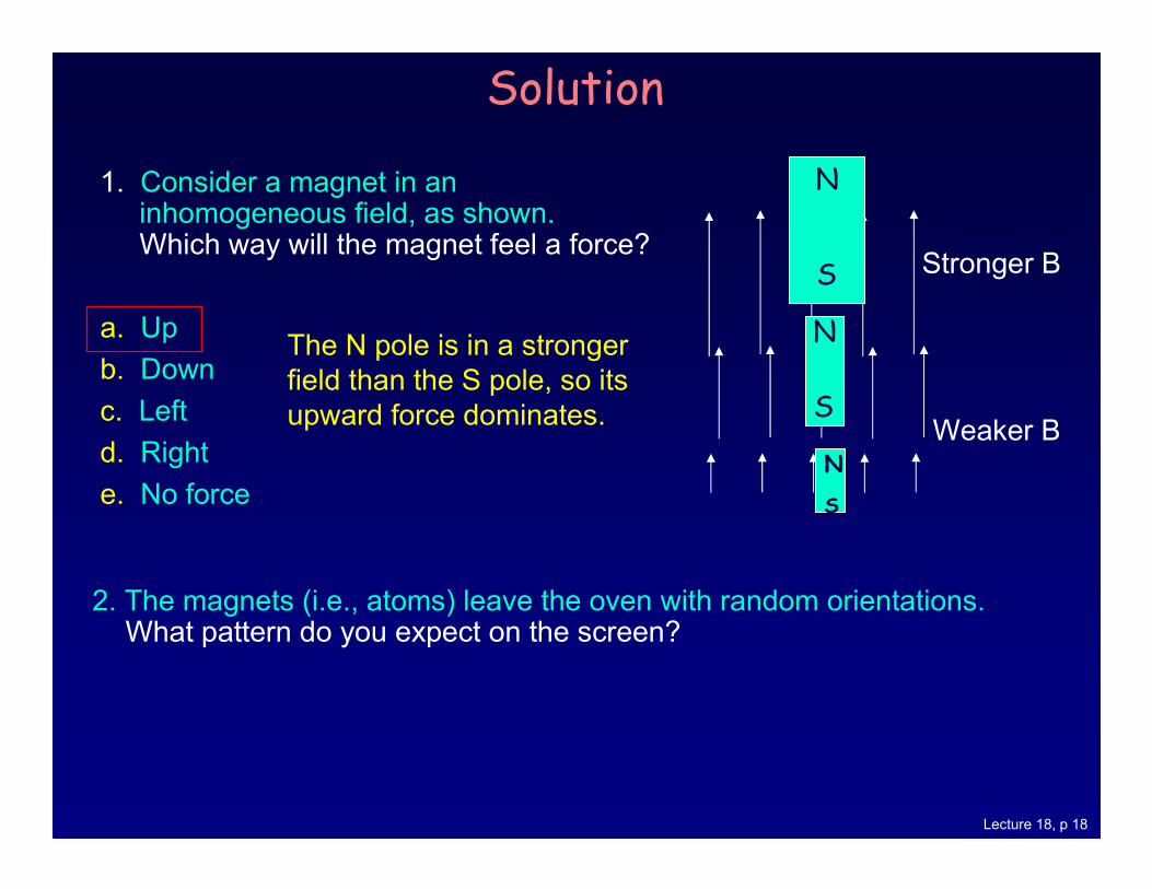
Solution

1. Consider a magnet in an inhomogeneous field, as shown. Which way will the magnet feel a force?

a. Up

b. Down

c. Left

d. Right

e. No force

Stronger B

Weaker B

N

S

The N pole is in a stronger

field than the S pole, so its

upward force dominates.

N

S

N

S

Lecture 18, p 19

2. The magnets (i.e., atoms) leave the oven with random orientations.What pattern do you expect on the screen?

Solution

1. Consider a magnet in an inhomogeneous field, as shown. Which way will the magnet feel a force?

a. Up

b. Down

c. Left

d. Right

e. No force

Stronger B

Weaker B

N

S

The N pole is in a stronger

field than the S pole, so its

upward force dominates.

B

oven

We expect a blob,

because the position

depends on the

random rotation angle.

Lecture 18, p 20

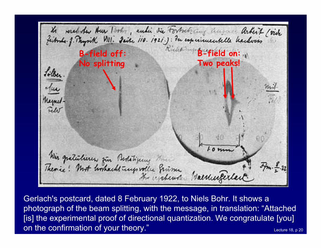
Gerlach's postcard, dated 8 February 1922, to Niels Bohr. It shows a

photograph of the beam splitting, with the message, in translation: “Attached

[is] the experimental proof of directional quantization. We congratulate [you]

on the confirmation of your theory.”

B-field off: No splitting

B-field on: Two peaks!

Lecture 18, p 21

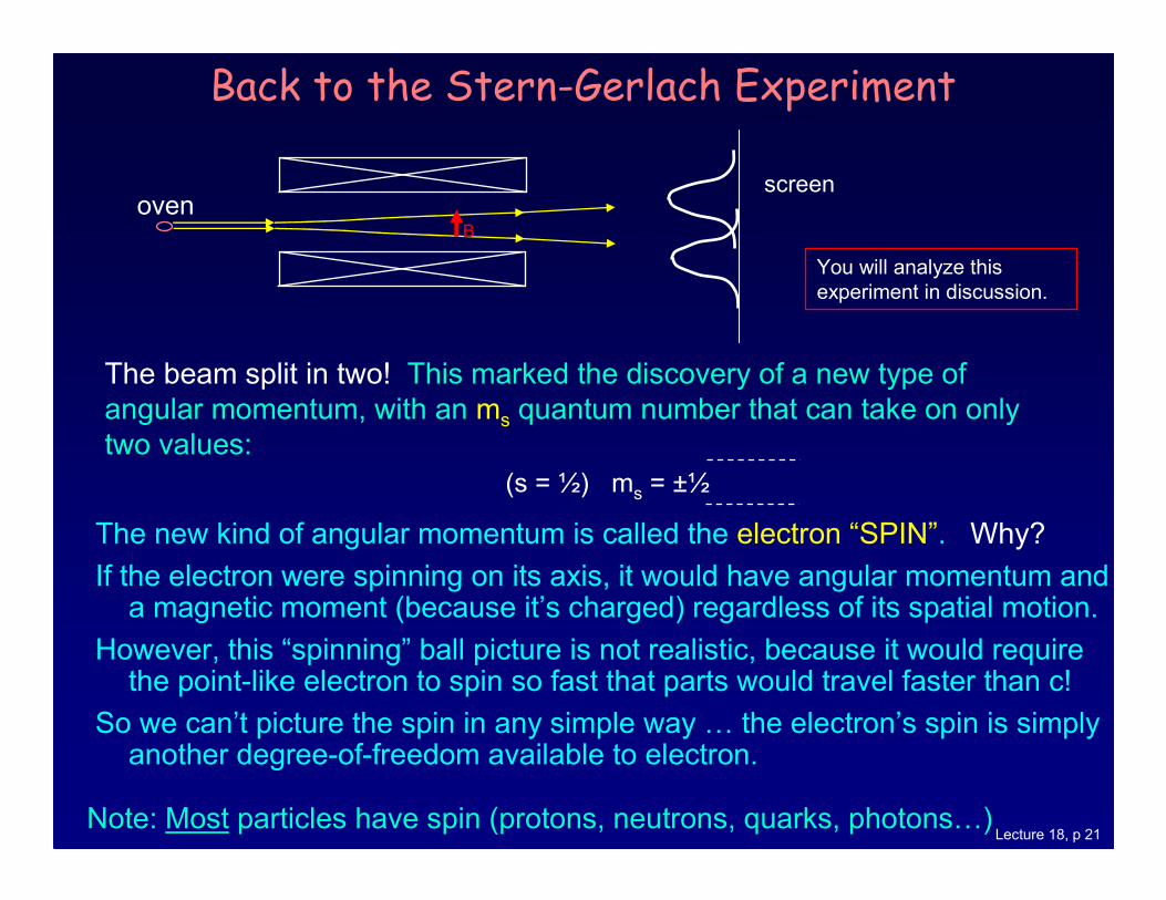
Back to the Stern-Gerlach Experiment

You will analyze this

experiment in discussion.

The beam split in two! This marked the discovery of a new type of

angular momentum, with an ms quantum number that can take on only

two values:

(s = ½) ms = ±½

screen

B

oven

Note: Most particles have spin (protons, neutrons, quarks, photonsO)

The new kind of angular momentum is called the electron “SPIN”. Why?

If the electron were spinning on its axis, it would have angular momentum and a magnetic moment (because it’s charged) regardless of its spatial motion.

However, this “spinning” ball picture is not realistic, because it would require the point-like electron to spin so fast that parts would travel faster than c!

So we can’t picture the spin in any simple way O the electron’s spin is simply another degree-of-freedom available to electron.

Lecture 18, p 22

Electron Spin

We need FOUR quantum numbers to specify the electronic state of a hydrogen atom.

n, l, ml, ms (where ms = -½ and +½)

Actually, the nucleus (a proton) also has spin, so we must specify its ms as well O

We’ll work some example problems next time.

Lecture 18, p 23

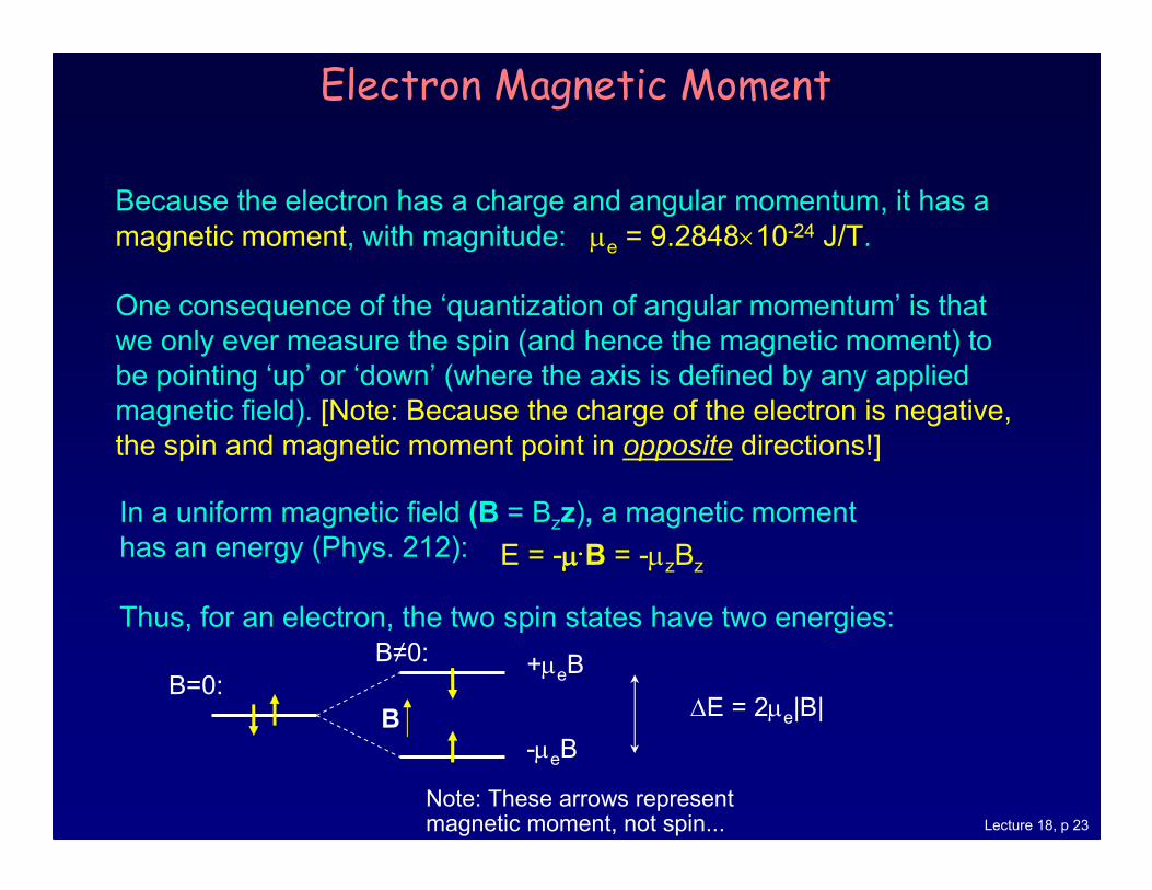
Electron Magnetic Moment

Because the electron has a charge and angular momentum, it has a

magnetic moment, with magnitude: µe = 9.2848×10-24 J/T.

One consequence of the ‘quantization of angular momentum’ is that

we only ever measure the spin (and hence the magnetic moment) to

be pointing ‘up’ or ‘down’ (where the axis is defined by any applied

magnetic field). [Note: Because the charge of the electron is negative,

the spin and magnetic moment point in opposite directions!]

E = -µµµµ....B = -µzBz

Note: These arrows represent magnetic moment, not spin...

∆E = 2µe|B|B=0:

B≠0: +µeB

-µeBB

In a uniform magnetic field (B = Bzz), a magnetic moment

has an energy (Phys. 212):

Thus, for an electron, the two spin states have two energies:

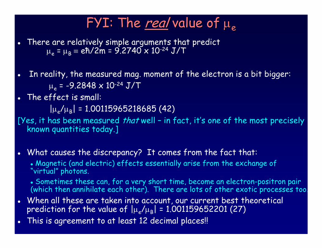
FYI: The FYI: The realreal value of value of µµee

� There are relatively simple arguments that predict µe = µB ≡ eћ/2m = 9.2740 x 10-24 J/T

� In reality, the measured mag. moment of the electron is a bit bigger:

µe = -9.2848 x 10-24 J/T

� The effect is small:

|µe/µB| = 1.00115965218685 (42)

[Yes, it has been measured that well – in fact, it’s one of the most precisely known quantities today.]

� What causes the discrepancy? It comes from the fact that:� Magnetic (and electric) effects essentially arise from the exchange of “virtual” photons.

� Sometimes these can, for a very short time, become an electron-positron pair (which then annihilate each other). There are lots of other exotic processes too.

� When all these are taken into account, our current best theoretical prediction for the value of |µe/µB| = 1.001159652201 (27)

� This is agreement to at least 12 decimal places!!

Lecture 18, p 25

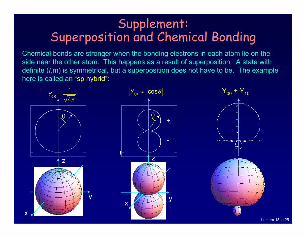
Supplement: Superposition and Chemical Bonding

z

x

y y

z

x

1

θ

0,0

1

4Y

π=

1

0

1

θ

1,0 cosY θ∝

+

-

Chemical bonds are stronger when the bonding electrons in each atom lie on the

side near the other atom. This happens as a result of superposition. A state with

definite (l,m) is symmetrical, but a superposition does not have to be. The example

here is called an “sp hybrid”:

Y00 + Y10

Lecture 18, p 26

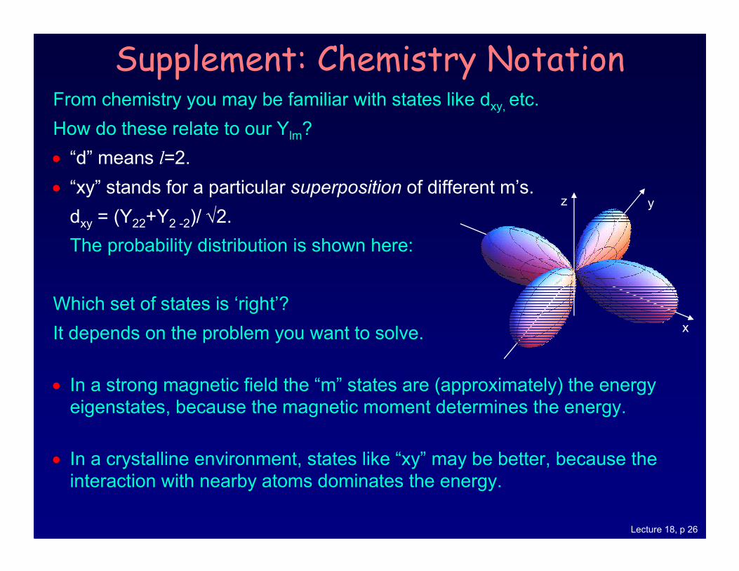
From chemistry you may be familiar with states like dxy, etc.

How do these relate to our Ylm?

• “d” means l=2.

• “xy” stands for a particular superposition of different m’s.

dxy = (Y22+Y2 -2)/ √2.

The probability distribution is shown here:

Which set of states is ‘right’?

It depends on the problem you want to solve.

• In a strong magnetic field the “m” states are (approximately) the energy

eigenstates, because the magnetic moment determines the energy.

• In a crystalline environment, states like “xy” may be better, because the

interaction with nearby atoms dominates the energy.

Supplement: Chemistry Notation

x

yz