Lecture 18. Autocorrelation & Dynamic Models Saw that may ...
171
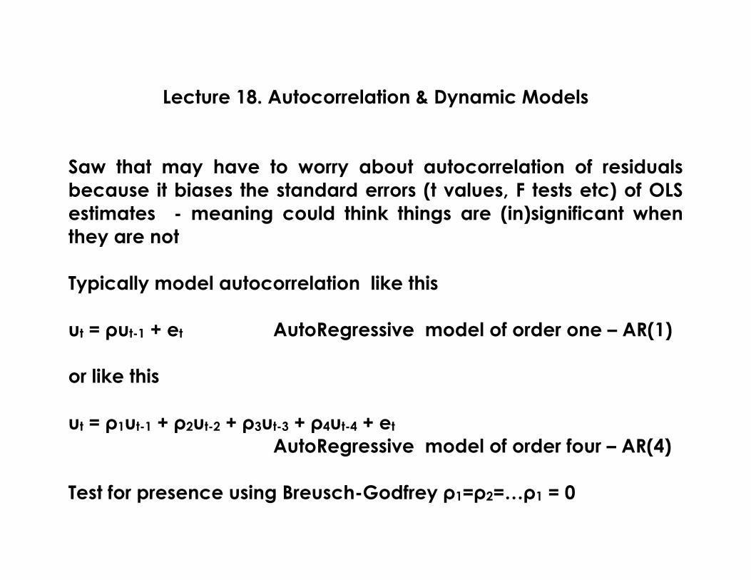
Lecture 18. Autocorrelation & Dynamic Models Saw that may have to worry about autocorrelation of residuals because it biases the standard errors (t values, F tests etc) of OLS estimates - meaning could think things are (in)significant when they are not Typically model autocorrelation like this u t = ρu t-1 + e t AutoRegressive model of order one – AR(1) or like this u t = ρ 1 u t-1 + ρ 2 u t-2 + ρ 3 u t-3 + ρ 4 u t-4 + e t AutoRegressive model of order four – AR(4) Test for presence using Breusch-Godfrey ρ 1 =ρ 2 =…ρ 1 = 0
Transcript of Lecture 18. Autocorrelation & Dynamic Models Saw that may ...
Lecture 18. Autocorrelation & Dynamic Models
Saw that may have to worry about autocorrelation of residuals because it biases the standard errors (t values, F tests etc) of OLS estimates - meaning could think things are (in)significant when they are not Typically model autocorrelation like this ut = ρut-1 + et AutoRegressive model of order one – AR(1) or like this ut = ρ1ut-1 + ρ2ut-2 + ρ3ut-3 + ρ4ut-4 + et
AutoRegressive model of order four – AR(4) Test for presence using Breusch-Godfrey ρ1=ρ2=…ρ1 = 0
Today: What to do about autocorrelation (change model, adjust standard errors) Estimating short and long run effects in dynamic models More problems when using time series data – stationarity What to do about stationarity

What to do about autocorrelation? If tests show it exists then

What to do about autocorrelation? If tests show it exists then
- try a different functional form,

What to do about autocorrelation? If tests show it exists then
- try a different functional form, - add/delete variables
What to do about autocorrelation? If tests show it exists then
- try a different functional form, - add/delete variables - increase the interval between observations (eg monthly to quarterly)
What to do about autocorrelation? If tests show it exists then
- try a different functional form, - add/delete variables - increase the interval between observations (eg monthly to quarterly)
- fix up the standard errors
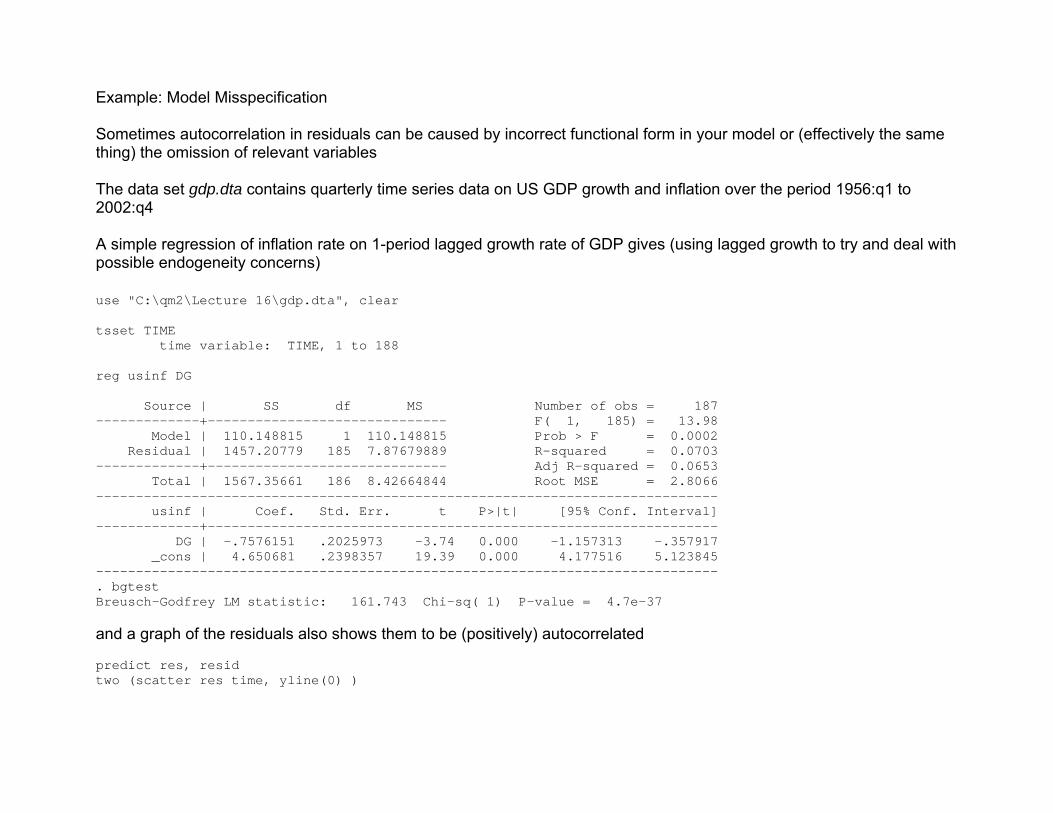
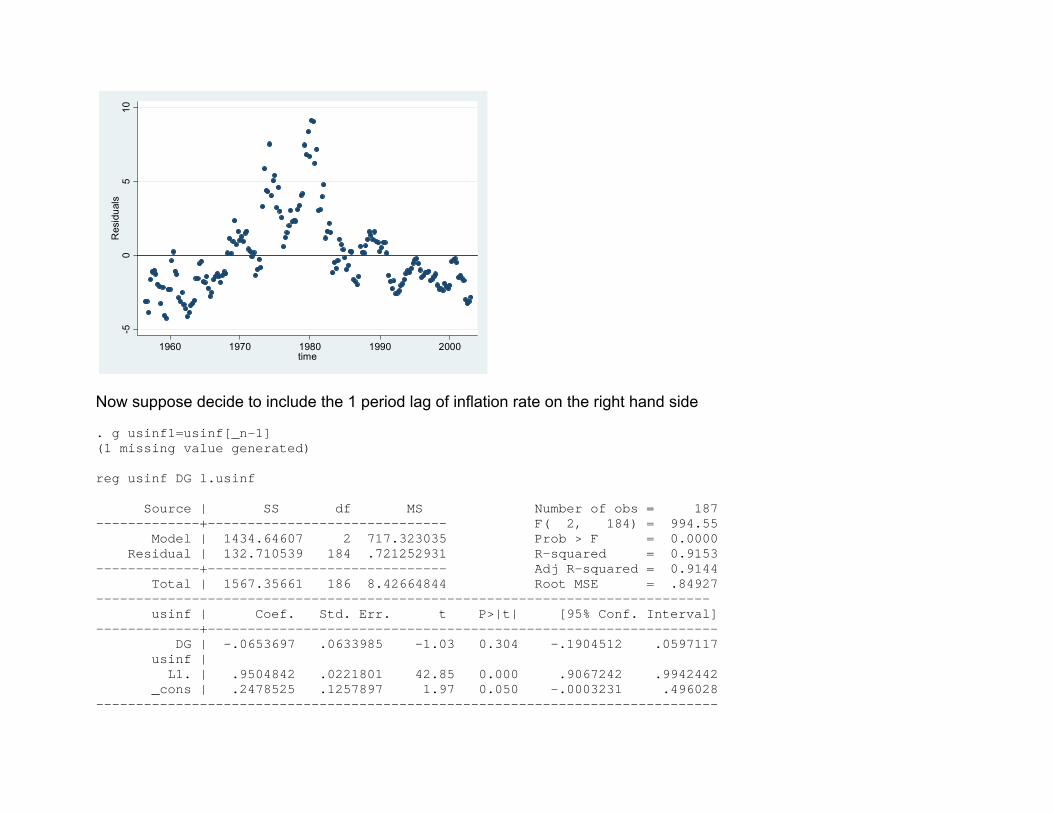
Example: Model Misspecification Sometimes autocorrelation in residuals can be caused by incorrect functional form in your model or (effectively the same thing) the omission of relevant variables The data set gdp.dta contains quarterly time series data on US GDP growth and inflation over the period 1956:q1 to 2002:q4 A simple regression of inflation rate on 1-period lagged growth rate of GDP gives (using lagged growth to try and deal with possible endogeneity concerns) use "C:\qm2\Lecture 16\gdp.dta", clear tsset TIME time variable: TIME, 1 to 188 reg usinf DG Source | SS df MS Number of obs = 187 -------------+------------------------------ F( 1, 185) = 13.98 Model | 110.148815 1 110.148815 Prob > F = 0.0002 Residual | 1457.20779 185 7.87679889 R-squared = 0.0703 -------------+------------------------------ Adj R-squared = 0.0653 Total | 1567.35661 186 8.42664844 Root MSE = 2.8066 ------------------------------------------------------------------------------ usinf | Coef. Std. Err. t P>|t| [95% Conf. Interval] -------------+---------------------------------------------------------------- DG | -.7576151 .2025973 -3.74 0.000 -1.157313 -.357917 _cons | 4.650681 .2398357 19.39 0.000 4.177516 5.123845 ------------------------------------------------------------------------------ . bgtest Breusch-Godfrey LM statistic: 161.743 Chi-sq( 1) P-value = 4.7e-37 and a graph of the residuals also shows them to be (positively) autocorrelated predict res, resid two (scatter res time, yline(0) )
-50
510
Res
idua
ls
1960 1970 1980 1990 2000time
Now suppose decide to include the 1 period lag of inflation rate on the right hand side . g usinf1=usinf[_n-1] (1 missing value generated) reg usinf DG l.usinf Source | SS df MS Number of obs = 187 -------------+------------------------------ F( 2, 184) = 994.55 Model | 1434.64607 2 717.323035 Prob > F = 0.0000 Residual | 132.710539 184 .721252931 R-squared = 0.9153 -------------+------------------------------ Adj R-squared = 0.9144 Total | 1567.35661 186 8.42664844 Root MSE = .84927 ----------------------------------------------------------------------------- usinf | Coef. Std. Err. t P>|t| [95% Conf. Interval] -------------+---------------------------------------------------------------- DG | -.0653697 .0633985 -1.03 0.304 -.1904512 .0597117 usinf | L1. | .9504842 .0221801 42.85 0.000 .9067242 .9942442 _cons | .2478525 .1257897 1.97 0.050 -.0003231 .496028 ------------------------------------------------------------------------------
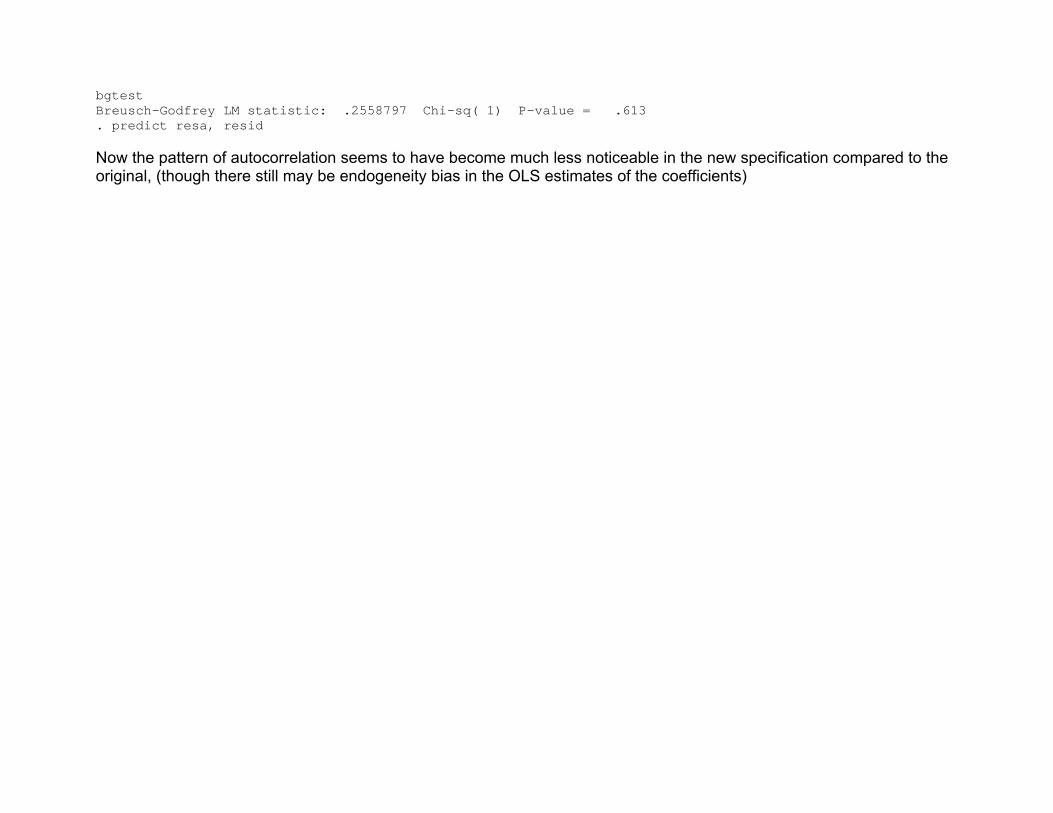
bgtest Breusch-Godfrey LM statistic: .2558797 Chi-sq( 1) P-value = .613 . predict resa, resid Now the pattern of autocorrelation seems to have become much less noticeable in the new specification compared to the original, (though there still may be endogeneity bias in the OLS estimates of the coefficients)
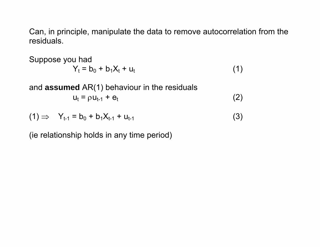
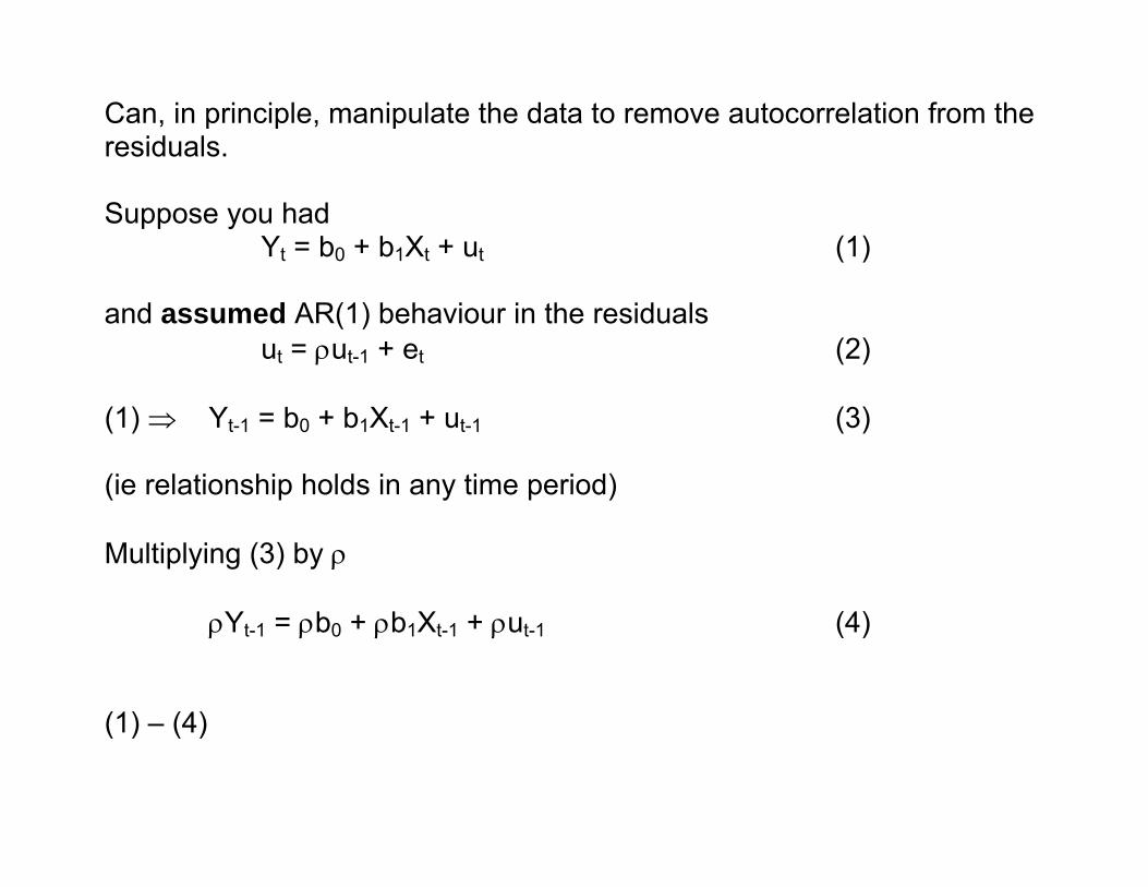
Can, in principle, manipulate the data to remove autocorrelation from the residuals.
Can, in principle, manipulate the data to remove autocorrelation from the residuals. Suppose you had Yt = b0 + b1Xt + ut (1) and assumed AR(1) behaviour in the residuals
ut = ρut-1 + et (2)
Can, in principle, manipulate the data to remove autocorrelation from the residuals. Suppose you had Yt = b0 + b1Xt + ut (1) and assumed AR(1) behaviour in the residuals
ut = ρut-1 + et (2) (1) ⇒ Yt-1 = b0 + b1Xt-1 + ut-1 (3) (ie relationship holds in any time period)
Can, in principle, manipulate the data to remove autocorrelation from the residuals. Suppose you had Yt = b0 + b1Xt + ut (1) and assumed AR(1) behaviour in the residuals
ut = ρut-1 + et (2) (1) ⇒ Yt-1 = b0 + b1Xt-1 + ut-1 (3) (ie relationship holds in any time period) Multiplying (3) by ρ
ρYt-1 = ρb0 + ρb1Xt-1 + ρut-1 (4)
(1) – (4)
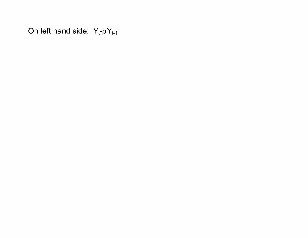
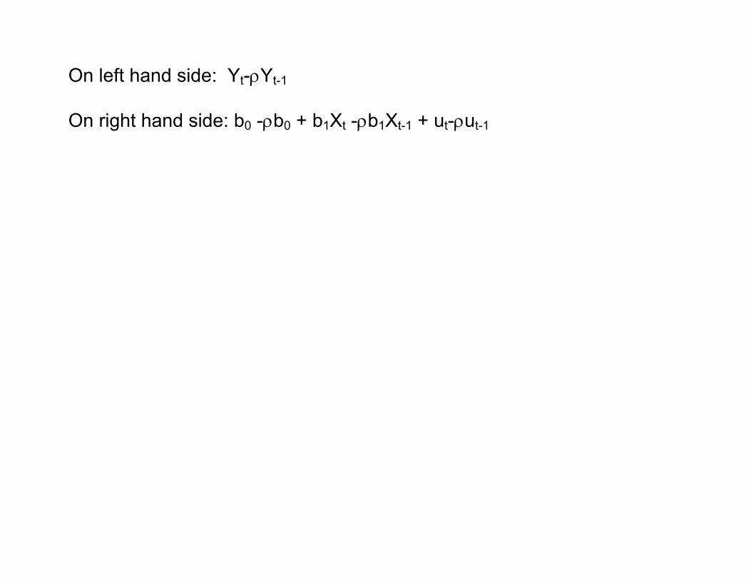
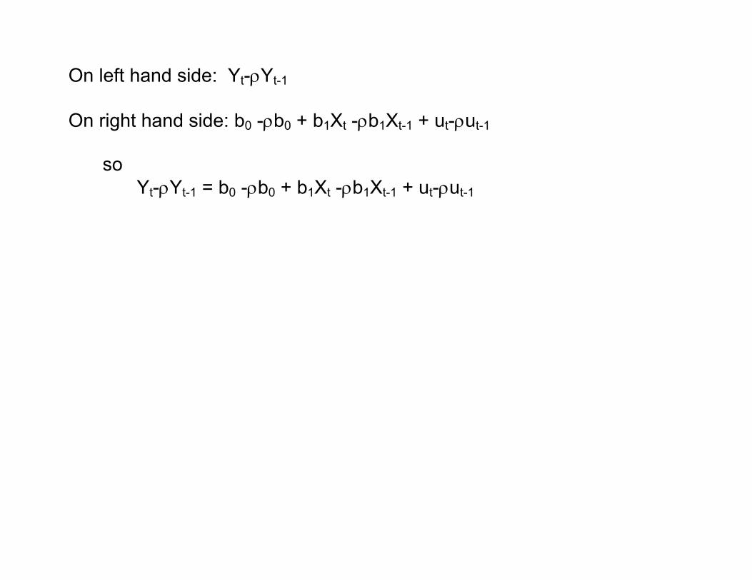
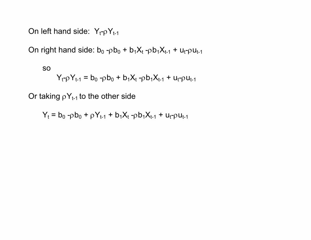
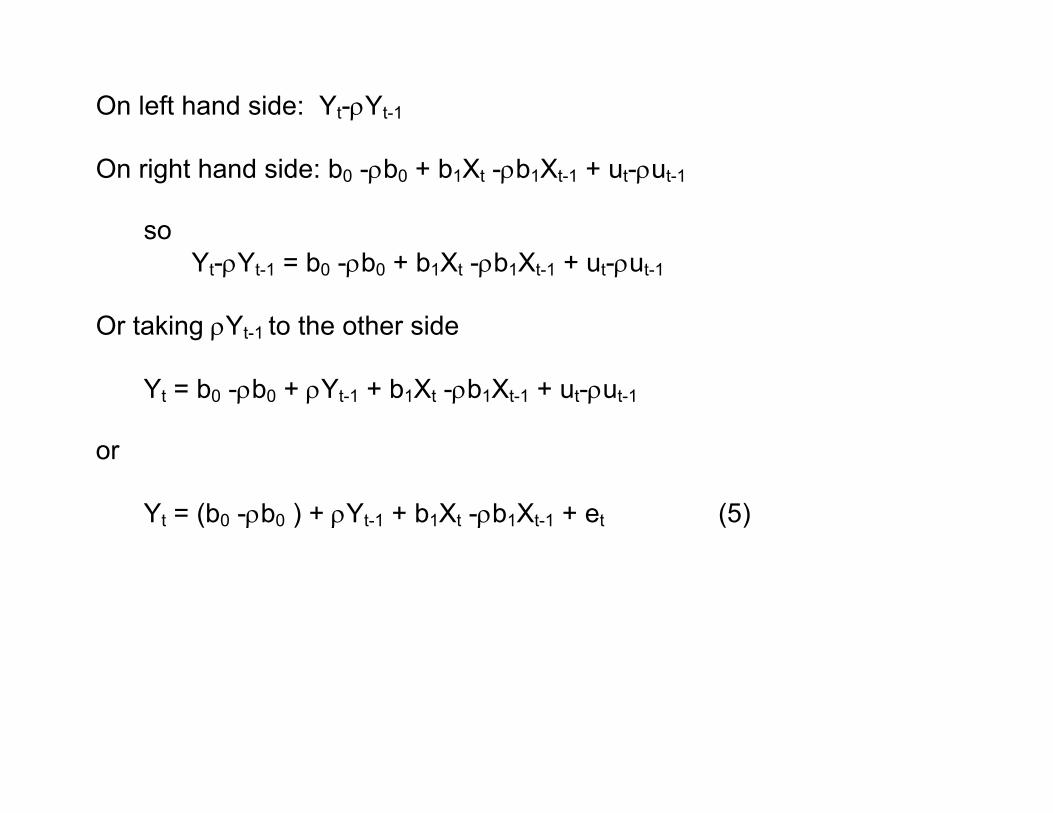
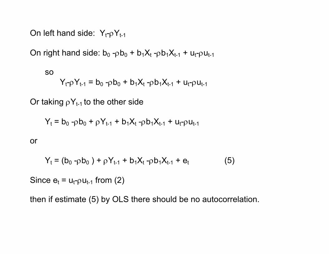
On left hand side: Yt-ρYt-1
On left hand side: Yt-ρYt-1
On right hand side: b0 -ρb0 + b1Xt -ρb1Xt-1 + ut-ρut-1
On left hand side: Yt-ρYt-1
On right hand side: b0 -ρb0 + b1Xt -ρb1Xt-1 + ut-ρut-1 so
Yt-ρYt-1 = b0 -ρb0 + b1Xt -ρb1Xt-1 + ut-ρut-1
On left hand side: Yt-ρYt-1
On right hand side: b0 -ρb0 + b1Xt -ρb1Xt-1 + ut-ρut-1 so
Yt-ρYt-1 = b0 -ρb0 + b1Xt -ρb1Xt-1 + ut-ρut-1
Or taking ρYt-1 to the other side
Yt = b0 -ρb0 + ρYt-1 + b1Xt -ρb1Xt-1 + ut-ρut-1
On left hand side: Yt-ρYt-1
On right hand side: b0 -ρb0 + b1Xt -ρb1Xt-1 + ut-ρut-1 so
Yt-ρYt-1 = b0 -ρb0 + b1Xt -ρb1Xt-1 + ut-ρut-1
Or taking ρYt-1 to the other side
Yt = b0 -ρb0 + ρYt-1 + b1Xt -ρb1Xt-1 + ut-ρut-1 or
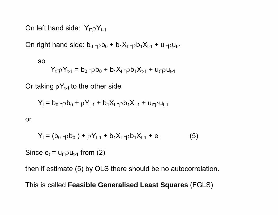
Yt = (b0 -ρb0 ) + ρYt-1 + b1Xt -ρb1Xt-1 + et (5)
On left hand side: Yt-ρYt-1
On right hand side: b0 -ρb0 + b1Xt -ρb1Xt-1 + ut-ρut-1 so
Yt-ρYt-1 = b0 -ρb0 + b1Xt -ρb1Xt-1 + ut-ρut-1
Or taking ρYt-1 to the other side
Yt = b0 -ρb0 + ρYt-1 + b1Xt -ρb1Xt-1 + ut-ρut-1 or
Yt = (b0 -ρb0 ) + ρYt-1 + b1Xt -ρb1Xt-1 + et (5)
Since et = ut-ρut-1 from (2) then if estimate (5) by OLS there should be no autocorrelation.
On left hand side: Yt-ρYt-1
On right hand side: b0 -ρb0 + b1Xt -ρb1Xt-1 + ut-ρut-1 so
Yt-ρYt-1 = b0 -ρb0 + b1Xt -ρb1Xt-1 + ut-ρut-1
Or taking ρYt-1 to the other side
Yt = b0 -ρb0 + ρYt-1 + b1Xt -ρb1Xt-1 + ut-ρut-1 or
Yt = (b0 -ρb0 ) + ρYt-1 + b1Xt -ρb1Xt-1 + et (5)
Since et = ut-ρut-1 from (2) then if estimate (5) by OLS there should be no autocorrelation. This is called Feasible Generalised Least Squares (FGLS)

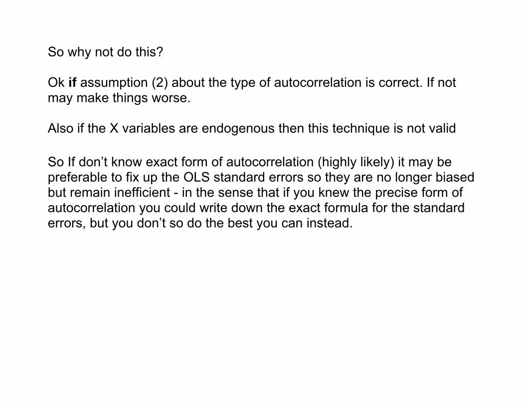
So why not do this?
So why not do this? Ok if assumption (2) about the type of autocorrelation is correct. If not may make things worse.
So why not do this? Ok if assumption (2) about the type of autocorrelation is correct. If not may make things worse. Also if the X variables are endogenous then this technique is not valid
So why not do this? Ok if assumption (2) about the type of autocorrelation is correct. If not may make things worse. Also if the X variables are endogenous then this technique is not valid
So If don’t know exact form of autocorrelation (highly likely) it may be preferable to fix up the OLS standard errors so they are no longer biased but remain inefficient - in the sense that if you knew the precise form of autocorrelation you could write down the exact formula for the standard errors, but you don’t so do the best you can instead.
So why not do this? Ok if assumption (2) about the type of autocorrelation is correct. If not may make things worse. Also if the X variables are endogenous then this technique is not valid
So If don’t know exact form of autocorrelation (highly likely) it may be preferable to fix up the OLS standard errors so they are no longer biased but remain inefficient - in the sense that if you knew the precise form of autocorrelation you could write down the exact formula for the standard errors, but you don’t so do the best you can instead. Newey-West standard errors do this and are valid in presence of lagged dependent variables and endogenous X variables if have large sample (ie fix-up is only valid asymptotically though it has been used on sample sizes of around 50).
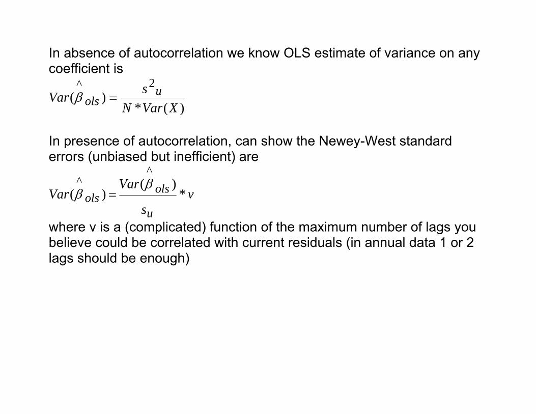
In absence of autocorrelation we know OLS estimate of variance on any coefficient is
)(*)(
2^
XVarNsVar u
ols =β
In presence of autocorrelation, can show the Newey-West standard errors (unbiased but inefficient) are
vs
VarVar
u
olsols *
)()(
^^ ββ =
where v is a (complicated) function of the maximum number of lags you believe could be correlated with current residuals (in annual data 1 or 2 lags should be enough)
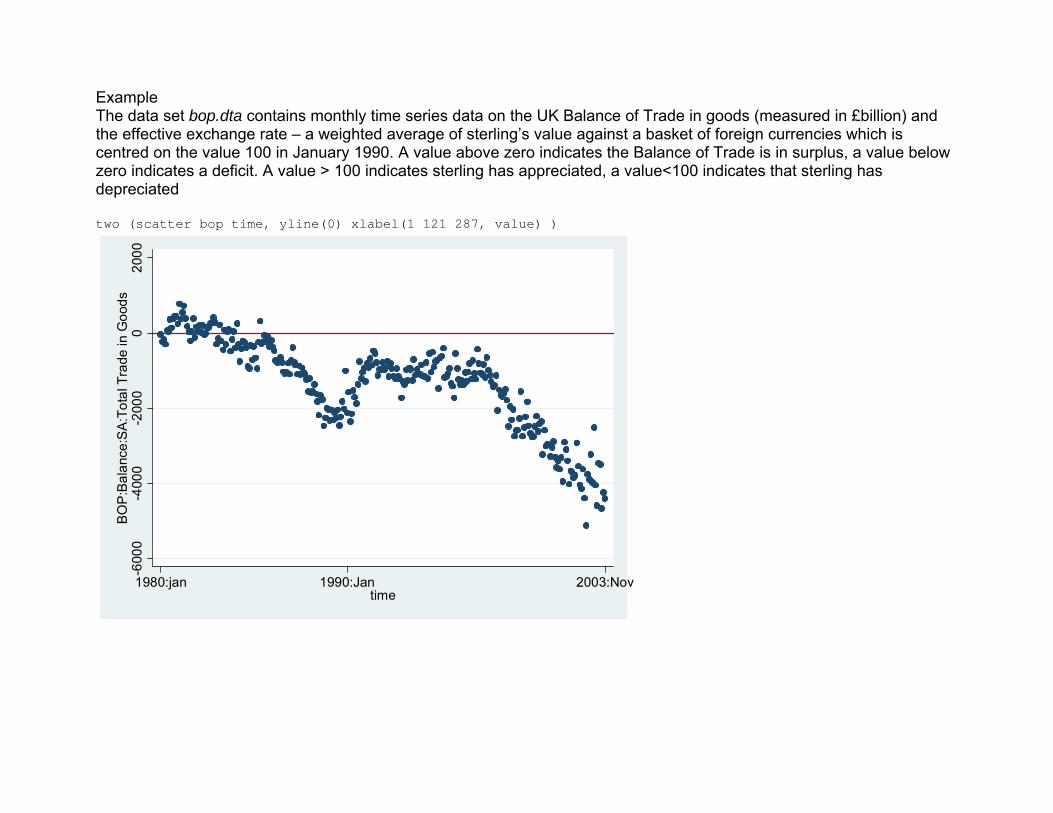
Example The data set bop.dta contains monthly time series data on the UK Balance of Trade in goods (measured in £billion) and the effective exchange rate – a weighted average of sterling’s value against a basket of foreign currencies which is centred on the value 100 in January 1990. A value above zero indicates the Balance of Trade is in surplus, a value below zero indicates a deficit. A value > 100 indicates sterling has appreciated, a value<100 indicates that sterling has depreciated two (scatter bop time, yline(0) xlabel(1 121 287, value) )
-600
0-4
000
-200
00
2000
BO
P:B
alan
ce:S
A:T
otal
Tra
de in
Goo
ds
1980:jan 1990:Jan 2003:Novtime
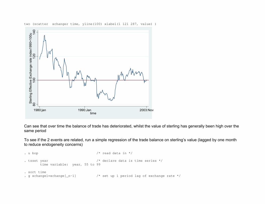
two (scatter xchanger time, yline(100) xlabel(1 121 287, value) )
8010
012
014
0S
terli
ng E
ffect
ive
Exc
hang
e ra
te in
dex1
990=
100u
1980:jan 1990:Jan 2003:Novtime
Can see that over time the balance of trade has deteriorated, whilst the value of sterling has generally been high over the same period To see if the 2 events are related, run a simple regression of the trade balance on sterling’s value (lagged by one month to reduce endogeneity concerns) . u bop /* read data in */ . tsset year /* declare data is time series */ time variable: year, 55 to 99 . sort time . g xchange1=xchange[_n-1] /* set up 1 period lag of exchange rate */
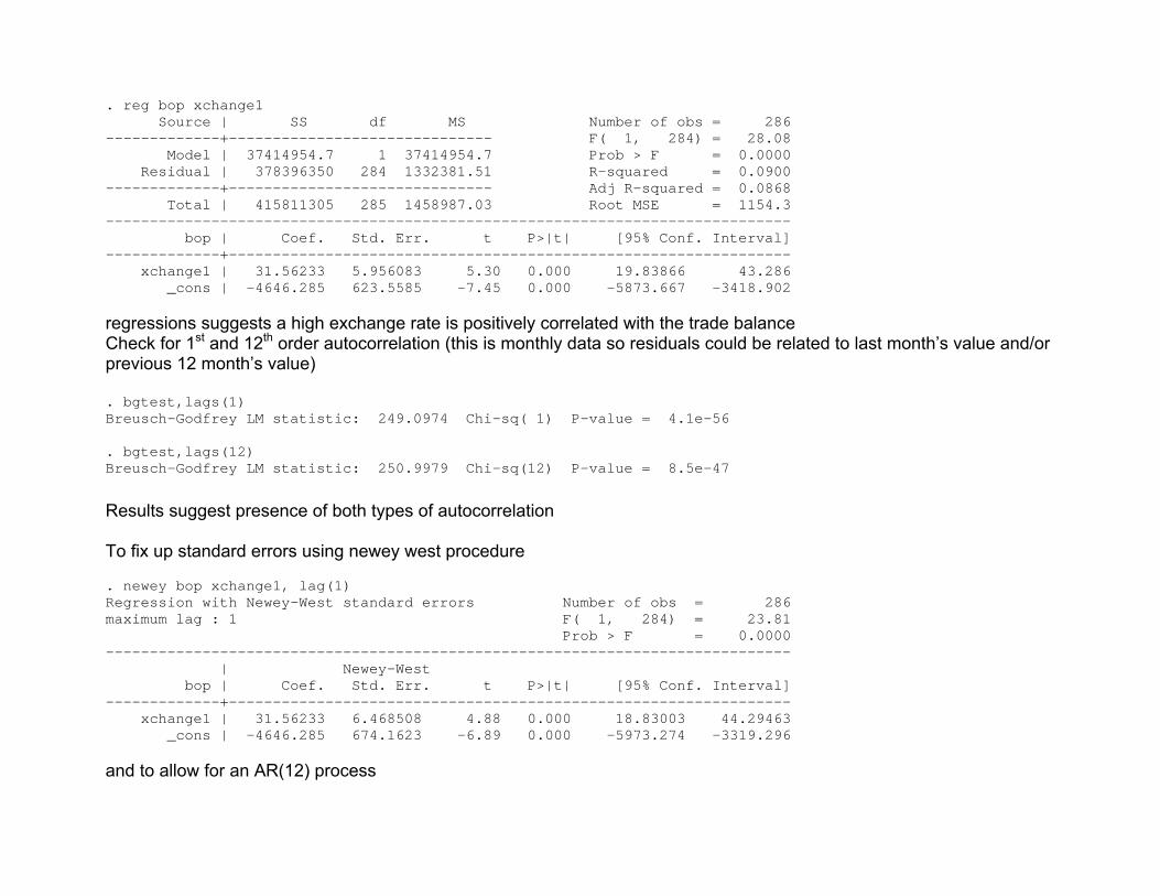
. reg bop xchange1 Source | SS df MS Number of obs = 286 -------------+------------------------------ F( 1, 284) = 28.08 Model | 37414954.7 1 37414954.7 Prob > F = 0.0000 Residual | 378396350 284 1332381.51 R-squared = 0.0900 -------------+------------------------------ Adj R-squared = 0.0868 Total | 415811305 285 1458987.03 Root MSE = 1154.3 ------------------------------------------------------------------------------ bop | Coef. Std. Err. t P>|t| [95% Conf. Interval] -------------+---------------------------------------------------------------- xchange1 | 31.56233 5.956083 5.30 0.000 19.83866 43.286 _cons | -4646.285 623.5585 -7.45 0.000 -5873.667 -3418.902 regressions suggests a high exchange rate is positively correlated with the trade balance Check for 1st and 12th order autocorrelation (this is monthly data so residuals could be related to last month’s value and/or previous 12 month’s value) . bgtest,lags(1) Breusch-Godfrey LM statistic: 249.0974 Chi-sq( 1) P-value = 4.1e-56 . bgtest,lags(12) Breusch-Godfrey LM statistic: 250.9979 Chi-sq(12) P-value = 8.5e-47
Results suggest presence of both types of autocorrelation To fix up standard errors using newey west procedure . newey bop xchange1, lag(1) Regression with Newey-West standard errors Number of obs = 286 maximum lag : 1 F( 1, 284) = 23.81 Prob > F = 0.0000 ------------------------------------------------------------------------------ | Newey-West bop | Coef. Std. Err. t P>|t| [95% Conf. Interval] -------------+---------------------------------------------------------------- xchange1 | 31.56233 6.468508 4.88 0.000 18.83003 44.29463 _cons | -4646.285 674.1623 -6.89 0.000 -5973.274 -3319.296 and to allow for an AR(12) process
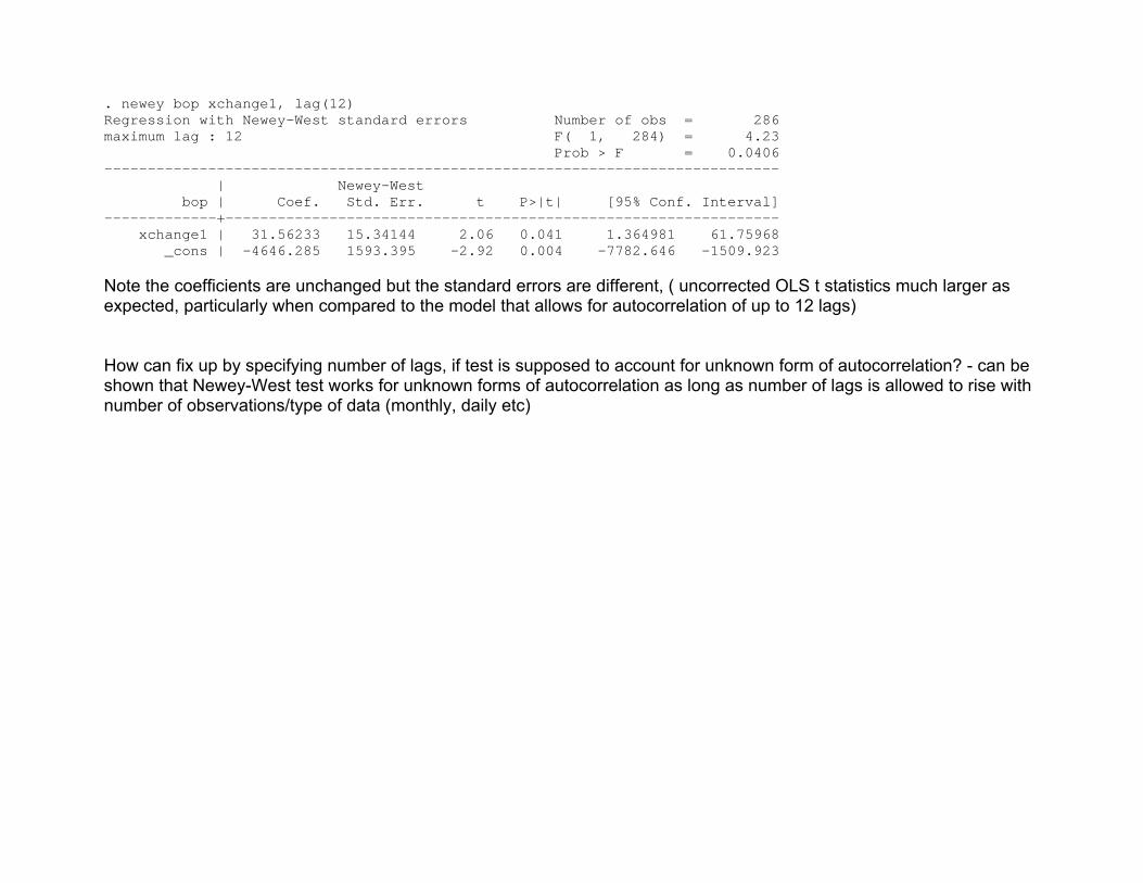
. newey bop xchange1, lag(12) Regression with Newey-West standard errors Number of obs = 286 maximum lag : 12 F( 1, 284) = 4.23 Prob > F = 0.0406 ------------------------------------------------------------------------------ | Newey-West bop | Coef. Std. Err. t P>|t| [95% Conf. Interval] -------------+---------------------------------------------------------------- xchange1 | 31.56233 15.34144 2.06 0.041 1.364981 61.75968 _cons | -4646.285 1593.395 -2.92 0.004 -7782.646 -1509.923 Note the coefficients are unchanged but the standard errors are different, ( uncorrected OLS t statistics much larger as expected, particularly when compared to the model that allows for autocorrelation of up to 12 lags) How can fix up by specifying number of lags, if test is supposed to account for unknown form of autocorrelation? - can be shown that Newey-West test works for unknown forms of autocorrelation as long as number of lags is allowed to rise with number of observations/type of data (monthly, daily etc)
Dynamic Models
Common in time series work to try and include lags of explanatory (and dependent) variables in a regression in order to account for belief that the influence of a variable could extend beyond the period in which any change occurred (“persistence” or “inertia” )
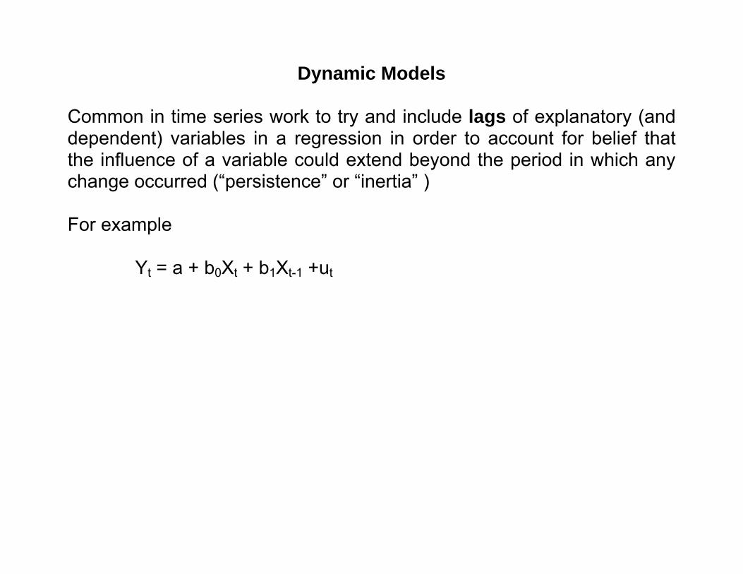
Dynamic Models
Common in time series work to try and include lags of explanatory (and dependent) variables in a regression in order to account for belief that the influence of a variable could extend beyond the period in which any change occurred (“persistence” or “inertia” ) For example
Yt = a + b0Xt + b1Xt-1 +ut
Dynamic Models
Common in time series work to try and include lags of explanatory (and dependent) variables in a regression in order to account for belief that the influence of a variable could extend beyond the period in which any change occurred (“persistence” or “inertia” ) For example
Yt = a + b0Xt + b1Xt-1 +ut is called a “distributed lag model of order 1” – since includes variables lagged at most by one period.
Dynamic Models
Common in time series work to try and include lags of explanatory (and dependent) variables in a regression in order to account for belief that the influence of a variable could extend beyond the period in which any change occurred (“persistence” or “inertia” ) For example
Yt = a + b0Xt + b1Xt-1 +ut is called a “distributed lag model of order 1” – since includes variables lagged at most by one period. The inclusion of lags turns the model from a static one into a dynamic one

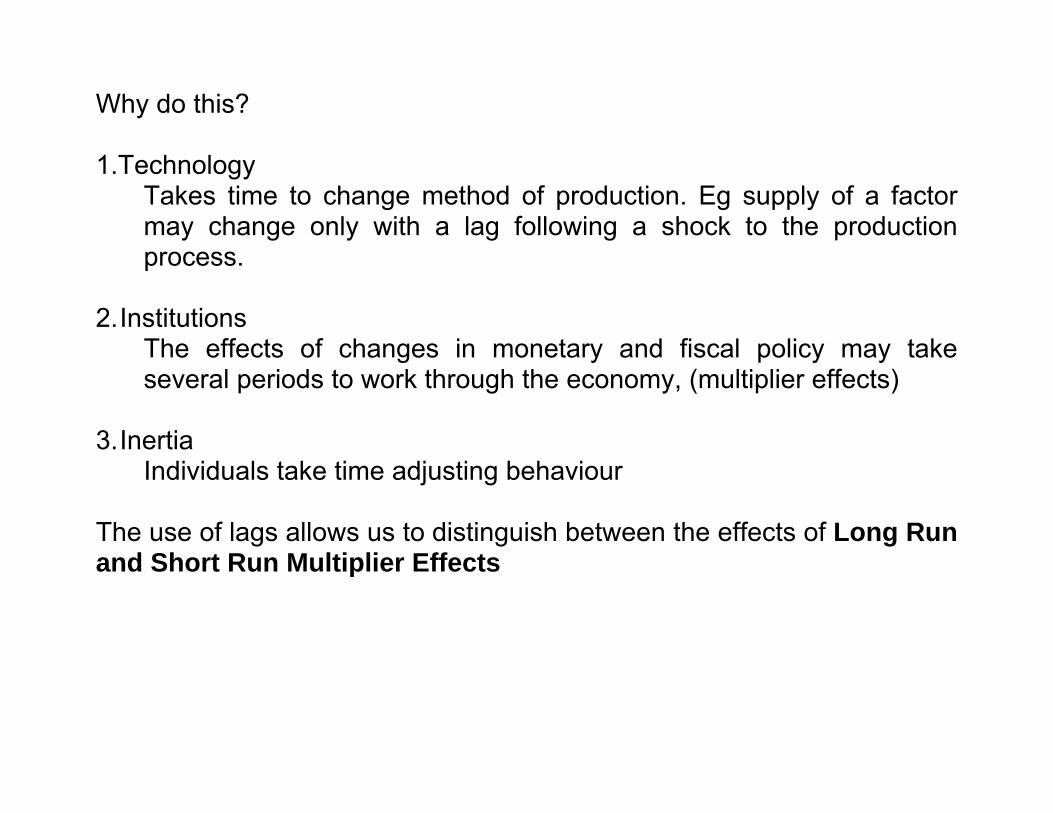
Why do this?
Why do this? 1. Technology
Takes time to change method of production. Eg supply of a factor may change only with a lag following a shock to the production process.
Why do this? 1. Technology
Takes time to change method of production. Eg supply of a factor may change only with a lag following a shock to the production process.
2. Institutions
The effects of changes in monetary and fiscal policy may take several periods to work through the economy, (multiplier effects)
3. Inertia
Individuals take time adjusting behaviour
Why do this? 1.Technology
Takes time to change method of production. Eg supply of a factor may change only with a lag following a shock to the production process.
2. Institutions
The effects of changes in monetary and fiscal policy may take several periods to work through the economy, (multiplier effects)
3. Inertia
Individuals take time adjusting behaviour The use of lags allows us to distinguish between the effects of Long Run and Short Run Multiplier Effects
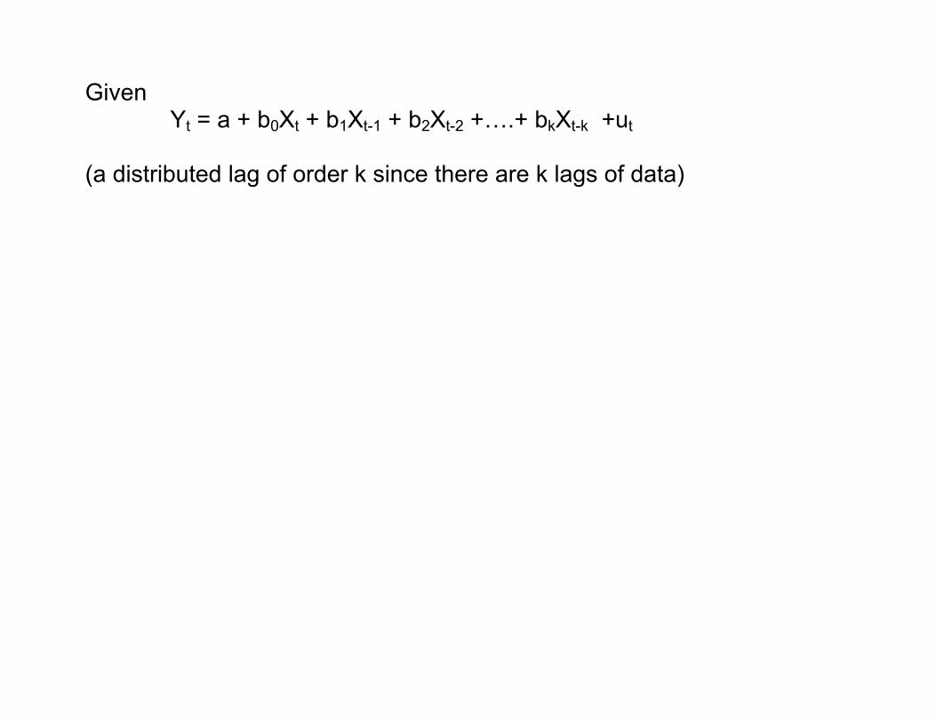
Given Yt = a + b0Xt + b1Xt-1 + b2Xt-2 +….+ bkXt-k +ut
(a distributed lag of order k since there are k lags of data)
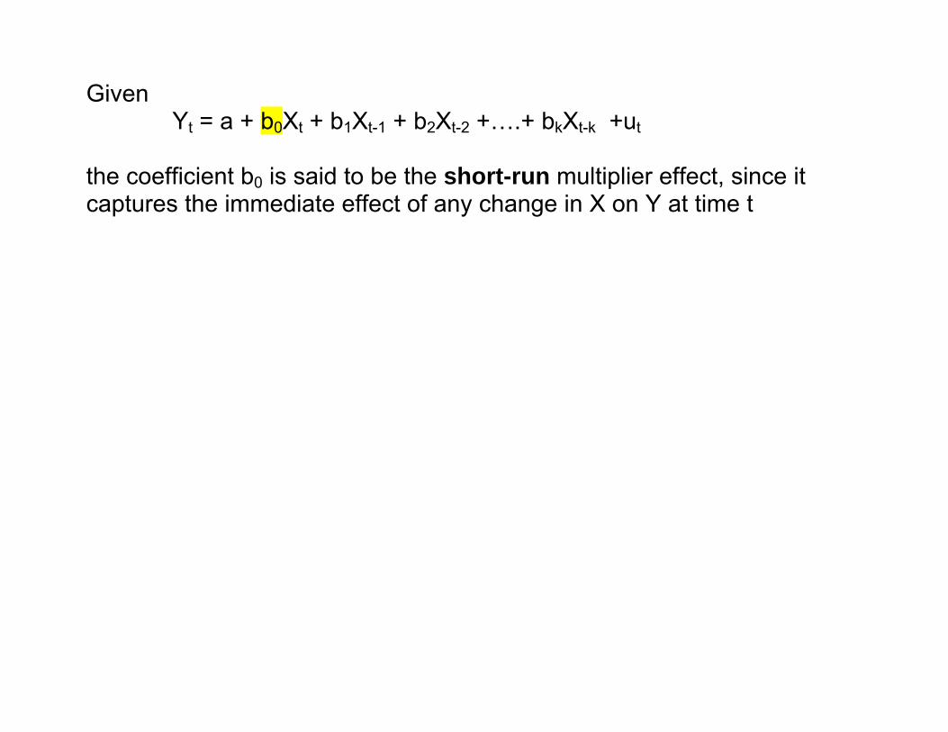
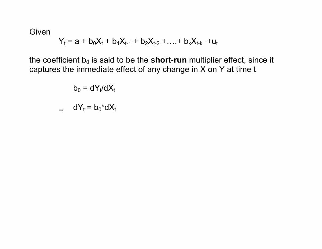
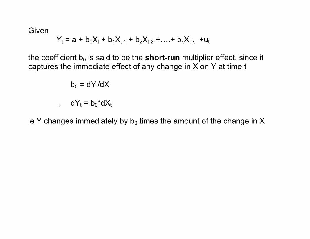
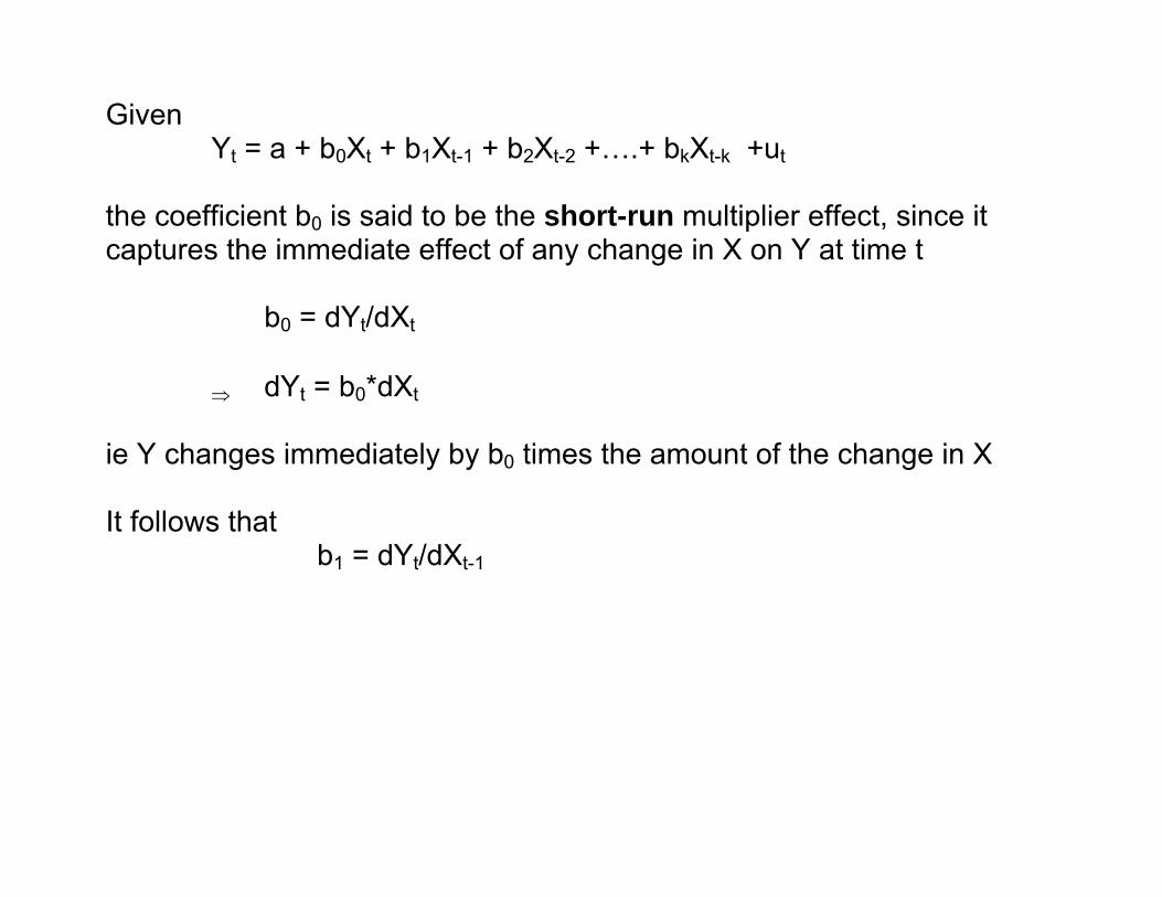
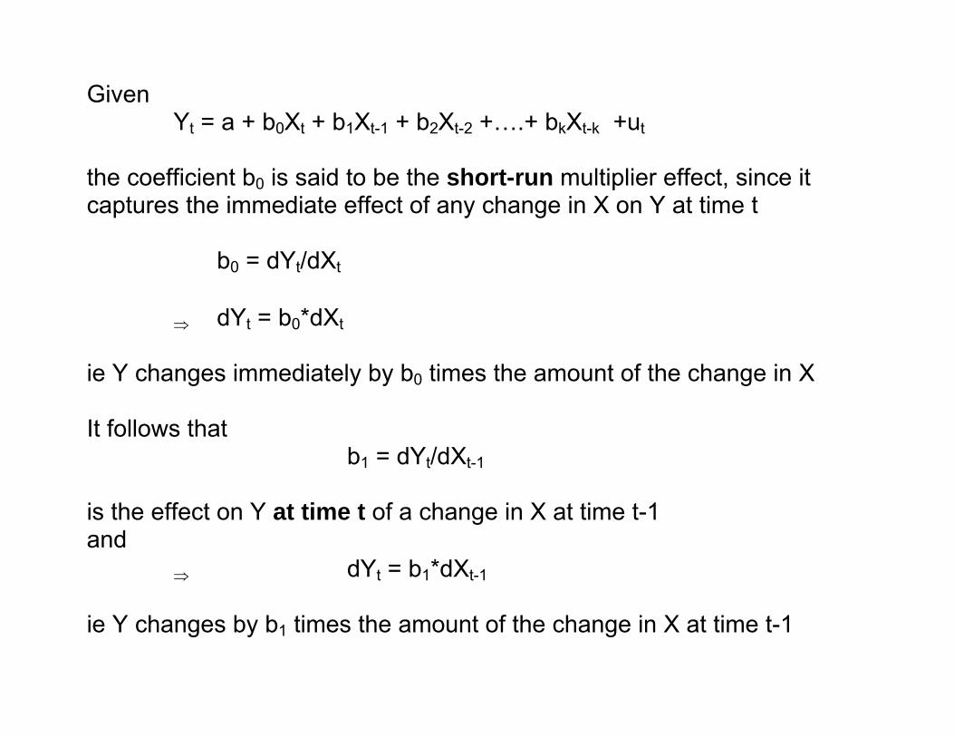
Given Yt = a + b0Xt + b1Xt-1 + b2Xt-2 +….+ bkXt-k +ut
the coefficient b0 is said to be the short-run multiplier effect, since it captures the immediate effect of any change in X on Y at time t
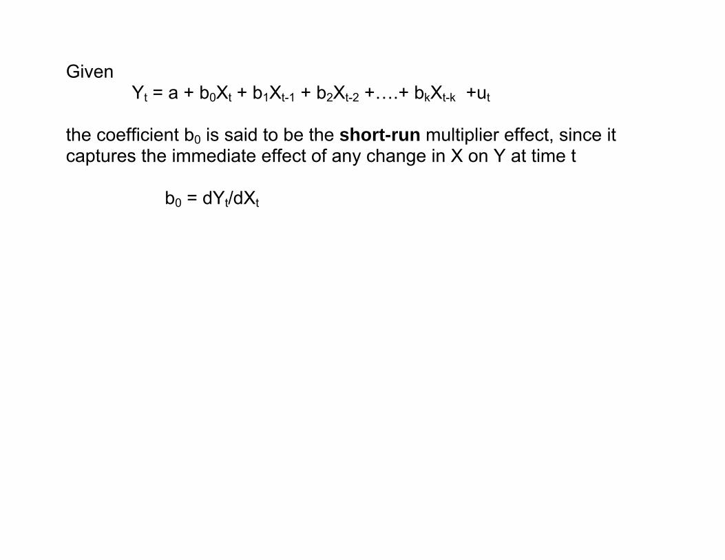
Given Yt = a + b0Xt + b1Xt-1 + b2Xt-2 +….+ bkXt-k +ut
the coefficient b0 is said to be the short-run multiplier effect, since it captures the immediate effect of any change in X on Y at time t b0 = dYt/dXt
Given Yt = a + b0Xt + b1Xt-1 + b2Xt-2 +….+ bkXt-k +ut
the coefficient b0 is said to be the short-run multiplier effect, since it captures the immediate effect of any change in X on Y at time t b0 = dYt/dXt
⇒ dYt = b0*dXt
Given Yt = a + b0Xt + b1Xt-1 + b2Xt-2 +….+ bkXt-k +ut
the coefficient b0 is said to be the short-run multiplier effect, since it captures the immediate effect of any change in X on Y at time t b0 = dYt/dXt
⇒ dYt = b0*dXt
ie Y changes immediately by b0 times the amount of the change in X
Given Yt = a + b0Xt + b1Xt-1 + b2Xt-2 +….+ bkXt-k +ut
the coefficient b0 is said to be the short-run multiplier effect, since it captures the immediate effect of any change in X on Y at time t b0 = dYt/dXt
⇒ dYt = b0*dXt
ie Y changes immediately by b0 times the amount of the change in X It follows that b1 = dYt/dXt-1
Given Yt = a + b0Xt + b1Xt-1 + b2Xt-2 +….+ bkXt-k +ut
the coefficient b0 is said to be the short-run multiplier effect, since it captures the immediate effect of any change in X on Y at time t b0 = dYt/dXt
⇒ dYt = b0*dXt
ie Y changes immediately by b0 times the amount of the change in X It follows that b1 = dYt/dXt-1 is the effect on Y at time t of a change in X at time t-1 and
⇒ dYt = b1*dXt-1
ie Y changes by b1 times the amount of the change in X at time t-1

Given Yt = a + b0Xt + b1Xt-1 + b2Xt-2 +….+ bkXt-k +ut
the coefficient b0 is said to be the short-run multiplier effect, since it captures the immediate effect of any change in X on Y at time t b0 = dYt/dXt
⇒ dYt = b0*dXt
ie Y changes immediately by b0 times the amount of the change in X It follows that b1 = dYt/dXt-1 is the effect on Y at time t of a change in X at time t-1 and
⇒ dYt = b1*dXt-1 ie Y changes by b1 times the amount of the change in X at time t-1 and so on for any other lag
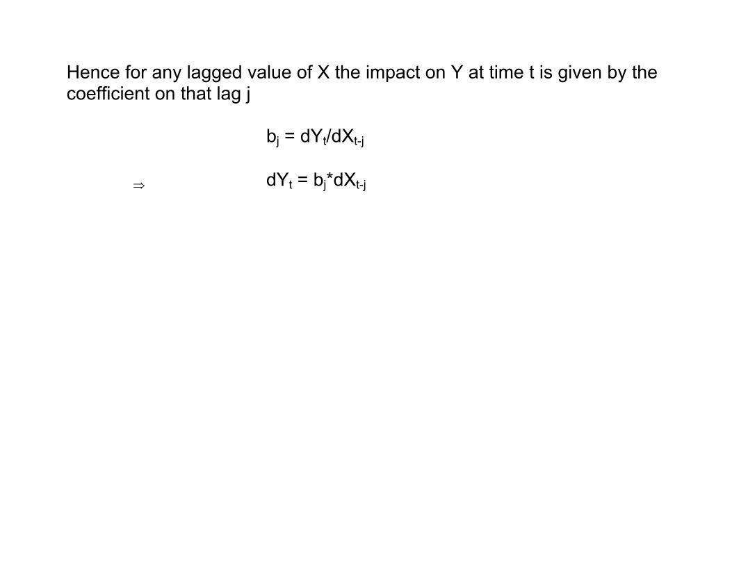
Hence for any lagged value of X the impact on Y at time t is given by the coefficient on that lag j bj = dYt/dXt-j
⇒ dYt = bj*dXt-j
Given this suppose X were increased by ΔX in every period (eg a new higher level of government spending), then in
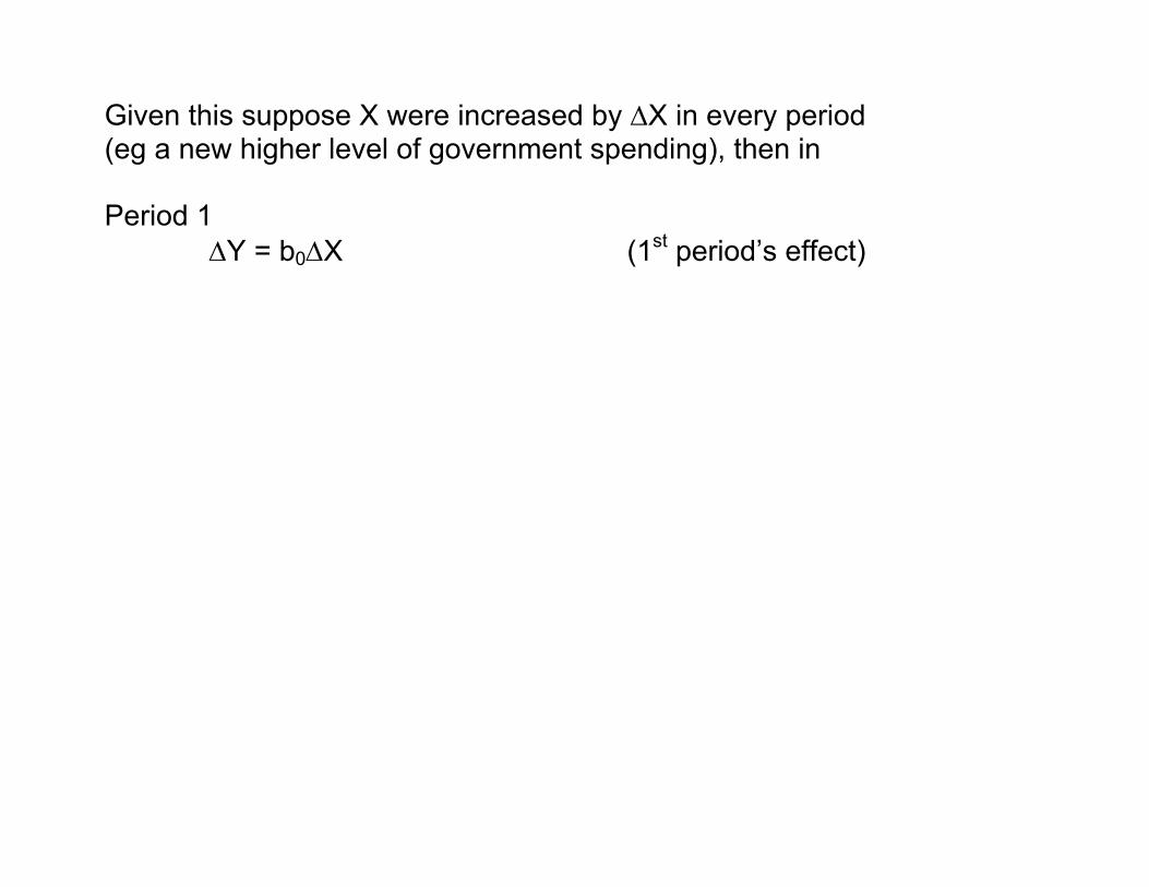
Given this suppose X were increased by ΔX in every period (eg a new higher level of government spending), then in Period 1 ΔY = b0ΔX (1st period’s effect)
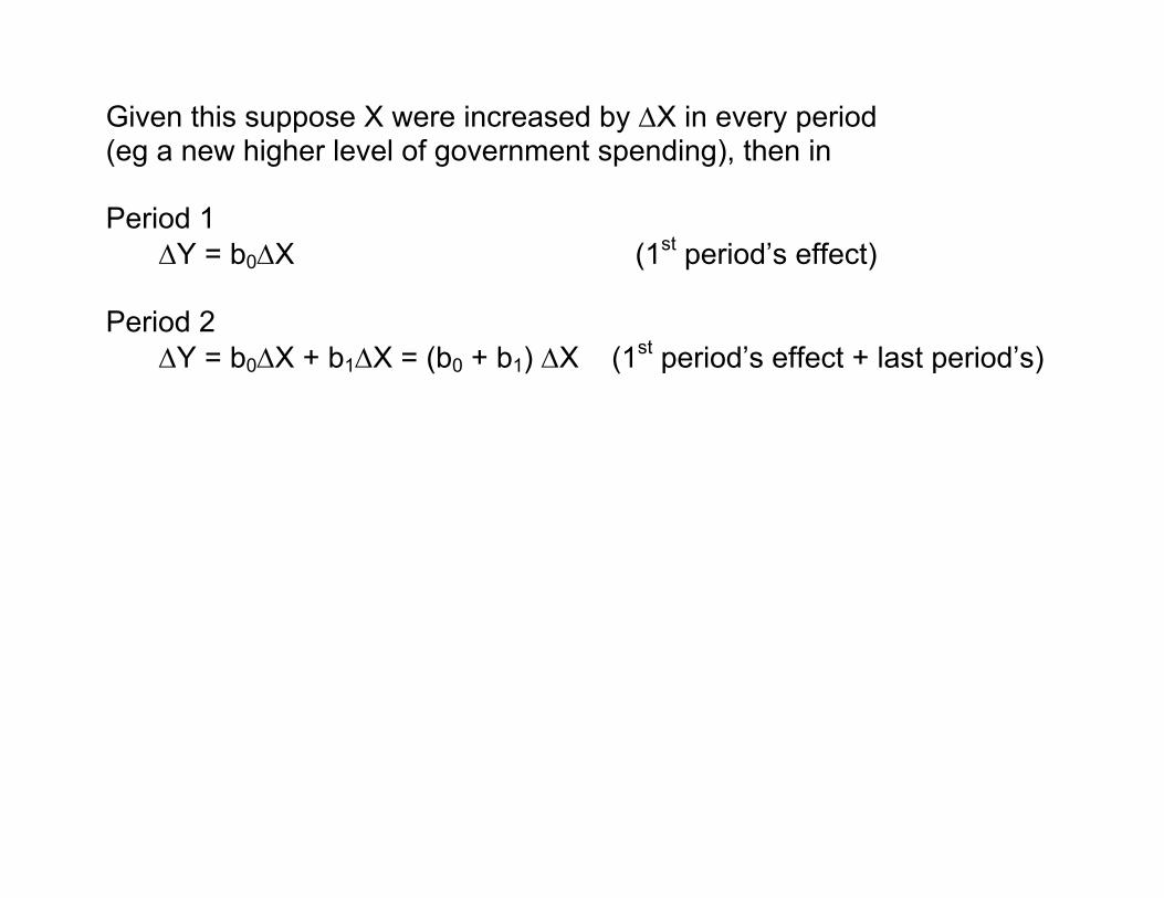
Given this suppose X were increased by ΔX in every period (eg a new higher level of government spending), then in Period 1 ΔY = b0ΔX (1st period’s effect) Period 2 ΔY = b0ΔX + b1ΔX = (b0 + b1) ΔX (1st period’s effect + last period’s)
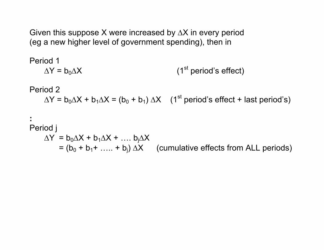
Given this suppose X were increased by ΔX in every period (eg a new higher level of government spending), then in Period 1 ΔY = b0ΔX (1st period’s effect) Period 2 ΔY = b0ΔX + b1ΔX = (b0 + b1) ΔX (1st period’s effect + last period’s) : Period j ΔY = b0ΔX + b1ΔX + …. bjΔX
= (b0 + b1+ ….. + bj) ΔX (cumulative effects from ALL periods)
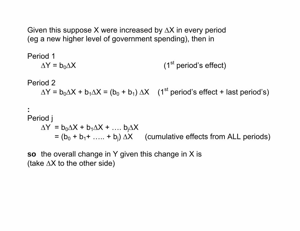
Given this suppose X were increased by ΔX in every period (eg a new higher level of government spending), then in Period 1 ΔY = b0ΔX (1st period’s effect) Period 2 ΔY = b0ΔX + b1ΔX = (b0 + b1) ΔX (1st period’s effect + last period’s) : Period j ΔY = b0ΔX + b1ΔX + …. bjΔX
= (b0 + b1+ ….. + bj) ΔX (cumulative effects from ALL periods) so the overall change in Y given this change in X is (take ΔX to the other side)
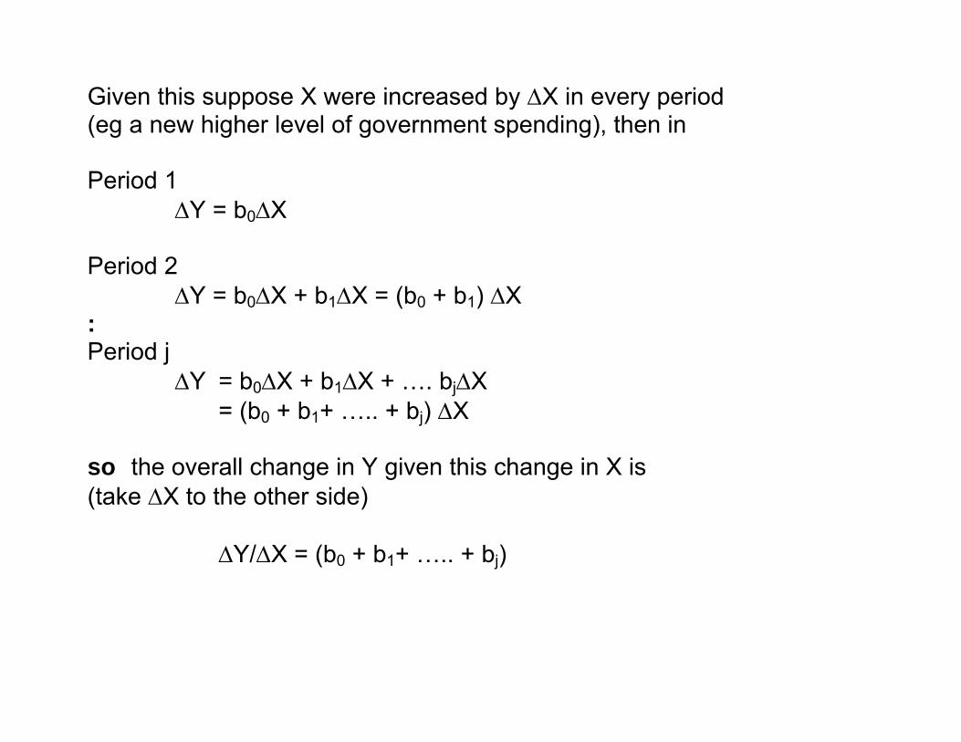
Given this suppose X were increased by ΔX in every period (eg a new higher level of government spending), then in Period 1 ΔY = b0ΔX Period 2 ΔY = b0ΔX + b1ΔX = (b0 + b1) ΔX : Period j ΔY = b0ΔX + b1ΔX + …. bjΔX
= (b0 + b1+ ….. + bj) ΔX so the overall change in Y given this change in X is (take ΔX to the other side) ΔY/ΔX = (b0 + b1+ ….. + bj)
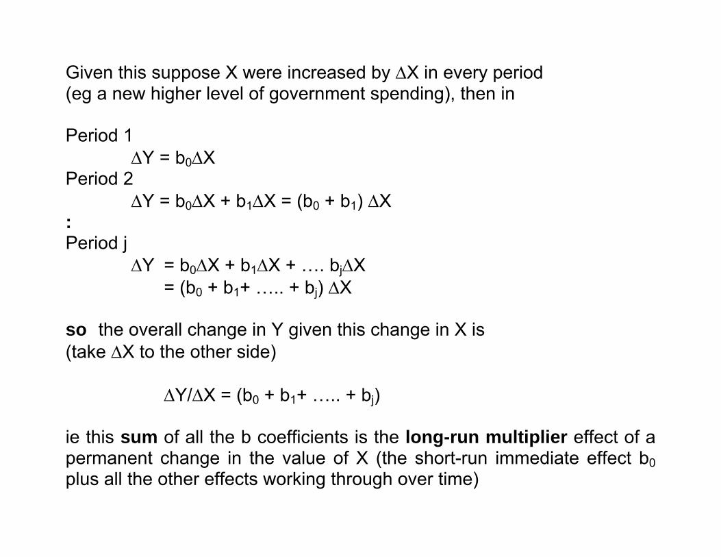
Given this suppose X were increased by ΔX in every period (eg a new higher level of government spending), then in Period 1 ΔY = b0ΔX Period 2 ΔY = b0ΔX + b1ΔX = (b0 + b1) ΔX : Period j ΔY = b0ΔX + b1ΔX + …. bjΔX
= (b0 + b1+ ….. + bj) ΔX so the overall change in Y given this change in X is (take ΔX to the other side) ΔY/ΔX = (b0 + b1+ ….. + bj) ie this sum of all the b coefficients is the long-run multiplier effect of a permanent change in the value of X (the short-run immediate effect b0 plus all the other effects working through over time)
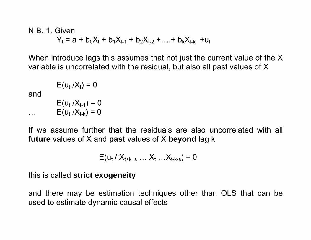
N.B. 1. Given Yt = a + b0Xt + b1Xt-1 + b2Xt-2 +….+ bkXt-k +ut
When introduce lags this assumes that not just the current value of the X variable is uncorrelated with the residual, but also all past values of X E(ut /Xt) = 0 and E(ut /Xt-1) = 0 … E(ut /Xt-k) = 0 If we assume further that the residuals are also uncorrelated with all future values of X and past values of X beyond lag k E(ut / Xt+k+s … Xt …Xt-k-s) = 0 this is called strict exogeneity and there may be estimation techniques other than OLS that can be used to estimate dynamic causal effects
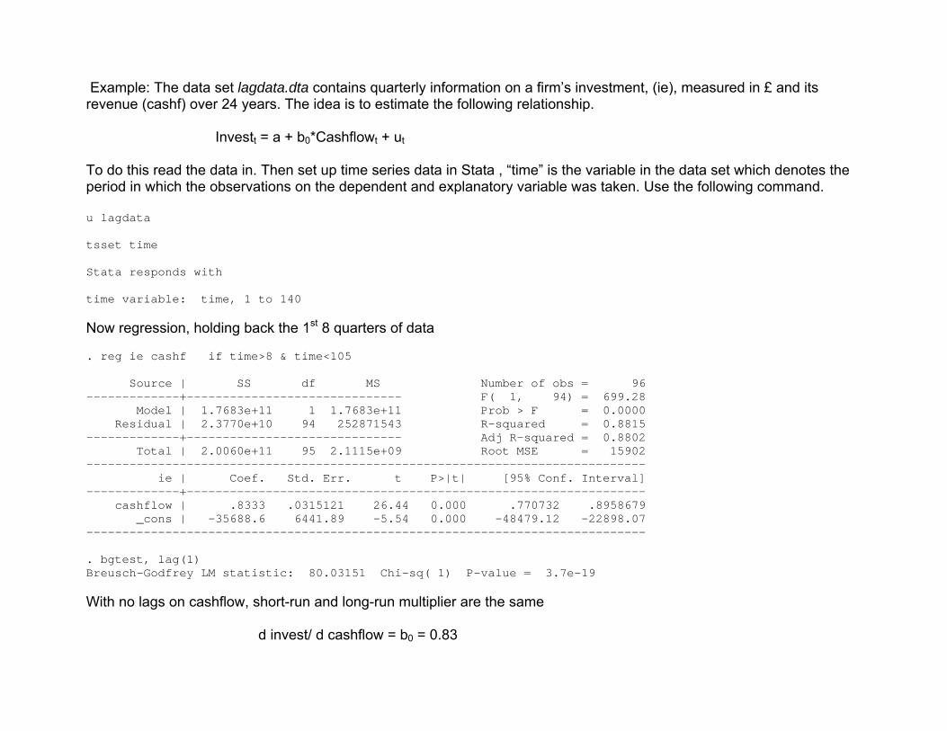
Example: The data set lagdata.dta contains quarterly information on a firm’s investment, (ie), measured in £ and its revenue (cashf) over 24 years. The idea is to estimate the following relationship. Investt = a + b0*Cashflowt + ut To do this read the data in. Then set up time series data in Stata , “time” is the variable in the data set which denotes the period in which the observations on the dependent and explanatory variable was taken. Use the following command. u lagdata tsset time Stata responds with time variable: time, 1 to 140 Now regression, holding back the 1st 8 quarters of data . reg ie cashf if time>8 & time<105 Source | SS df MS Number of obs = 96 -------------+------------------------------ F( 1, 94) = 699.28 Model | 1.7683e+11 1 1.7683e+11 Prob > F = 0.0000 Residual | 2.3770e+10 94 252871543 R-squared = 0.8815 -------------+------------------------------ Adj R-squared = 0.8802 Total | 2.0060e+11 95 2.1115e+09 Root MSE = 15902 ------------------------------------------------------------------------------ ie | Coef. Std. Err. t P>|t| [95% Conf. Interval] -------------+---------------------------------------------------------------- cashflow | .8333 .0315121 26.44 0.000 .770732 .8958679 _cons | -35688.6 6441.89 -5.54 0.000 -48479.12 -22898.07 ------------------------------------------------------------------------------ . bgtest, lag(1) Breusch-Godfrey LM statistic: 80.03151 Chi-sq( 1) P-value = 3.7e-19 With no lags on cashflow, short-run and long-run multiplier are the same d invest/ d cashflow = b0 = 0.83
so a £1 increase in revenue generates an immediate (and permanent) 83 pence increase in investment Note value of Breusch-Godfrey test indicates that there seems to be (1st order) autocorrelation in the data so standard errors are wrongly estimated, (but coefficients are unbiased).
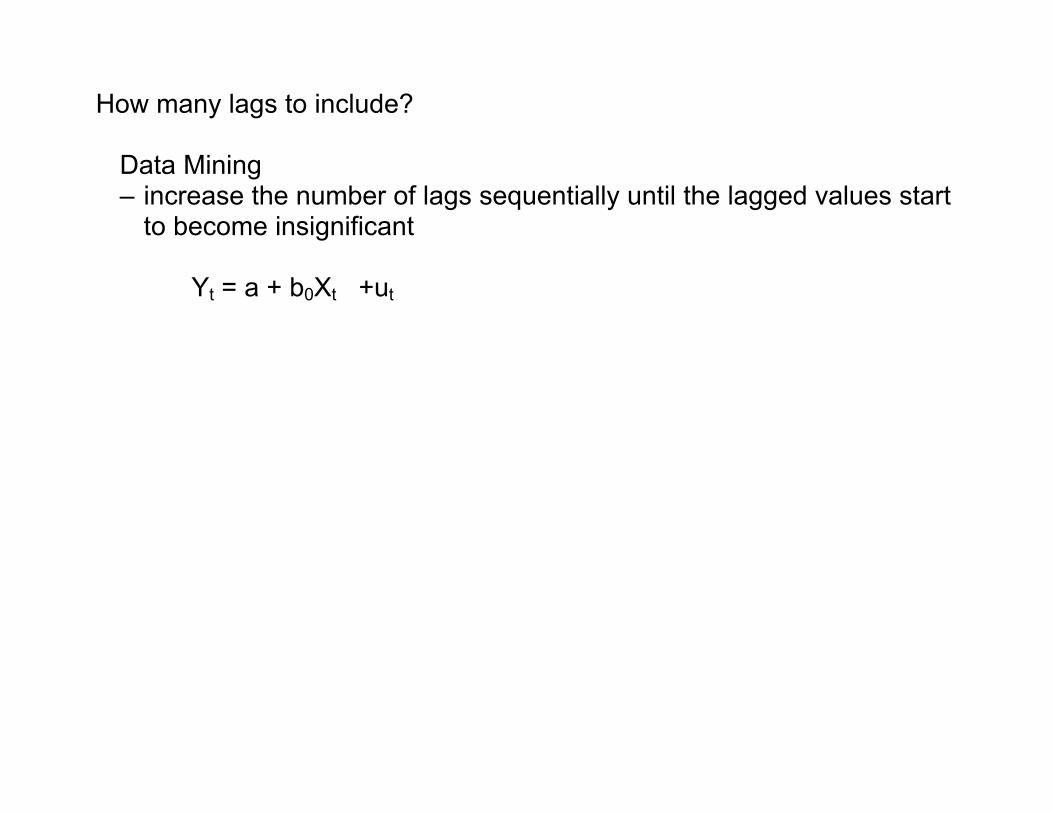
How many lags to include?
Data Mining – increase the number of lags sequentially until the lagged values start
to become insignificant
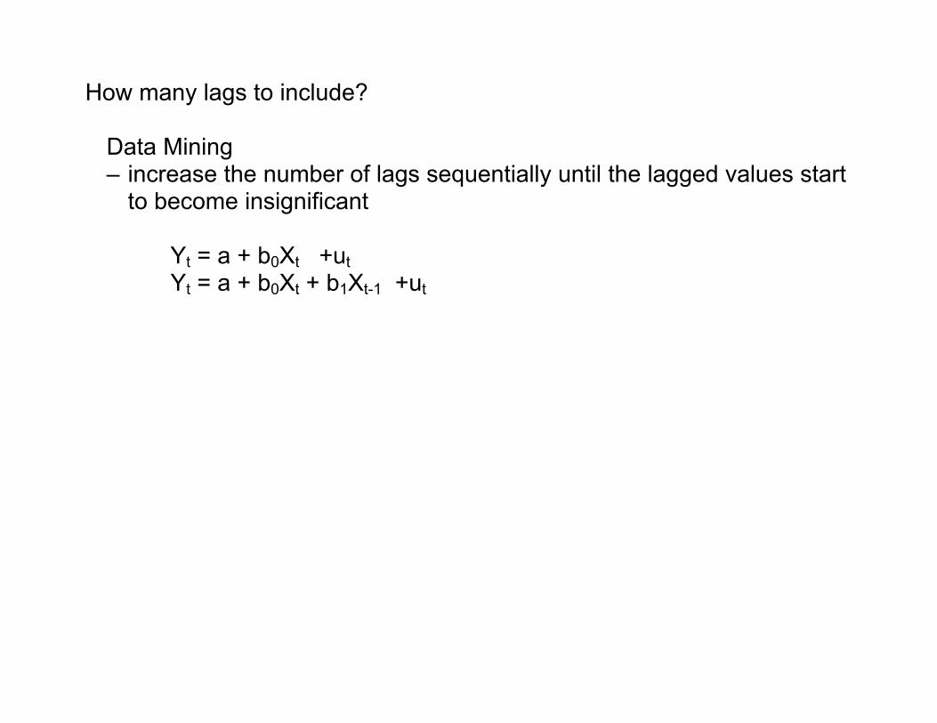
How many lags to include?
Data Mining – increase the number of lags sequentially until the lagged values start
to become insignificant
Yt = a + b0Xt +ut
How many lags to include?
Data Mining – increase the number of lags sequentially until the lagged values start
to become insignificant
Yt = a + b0Xt +ut Yt = a + b0Xt + b1Xt-1 +ut
How many lags to include?
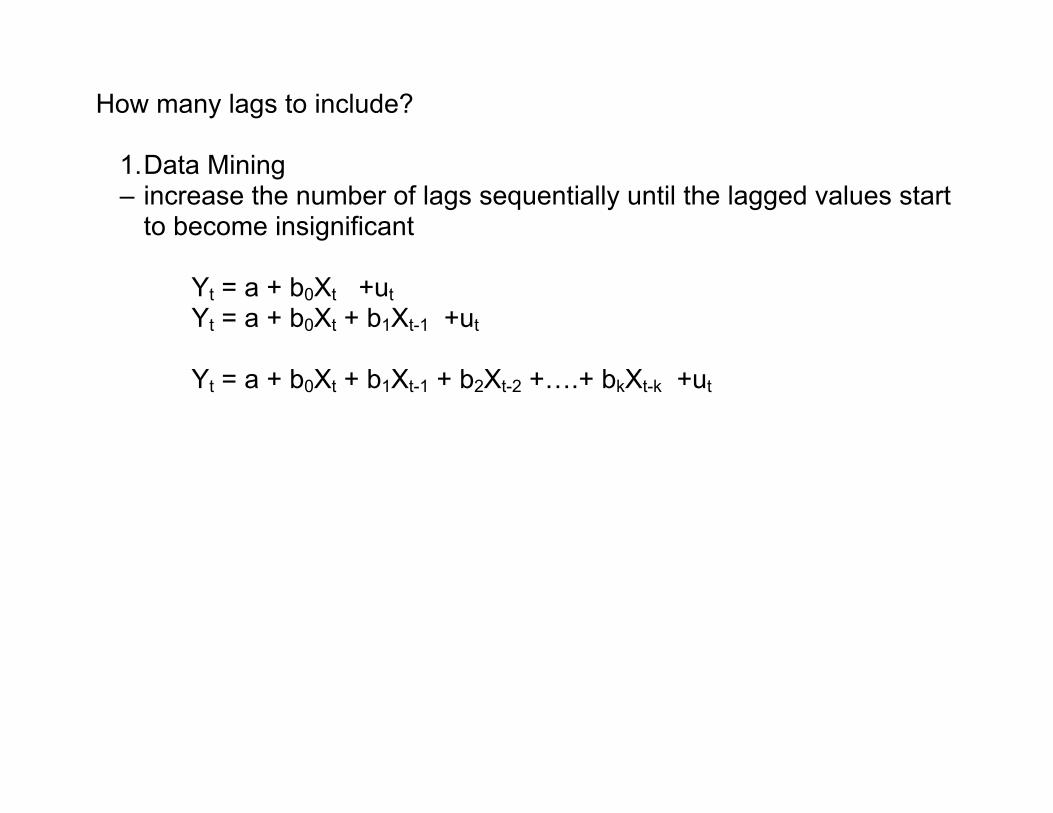
1. Data Mining – increase the number of lags sequentially until the lagged values start
to become insignificant
Yt = a + b0Xt +ut Yt = a + b0Xt + b1Xt-1 +ut
Yt = a + b0Xt + b1Xt-1 + b2Xt-2 +….+ bkXt-k +ut
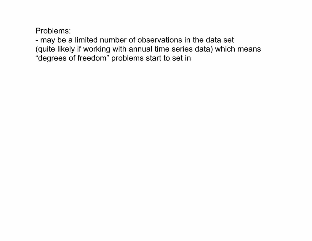
Problems: - may be a limited number of observations in the data set (quite likely if working with annual time series data) which means “degrees of freedom” problems start to set in
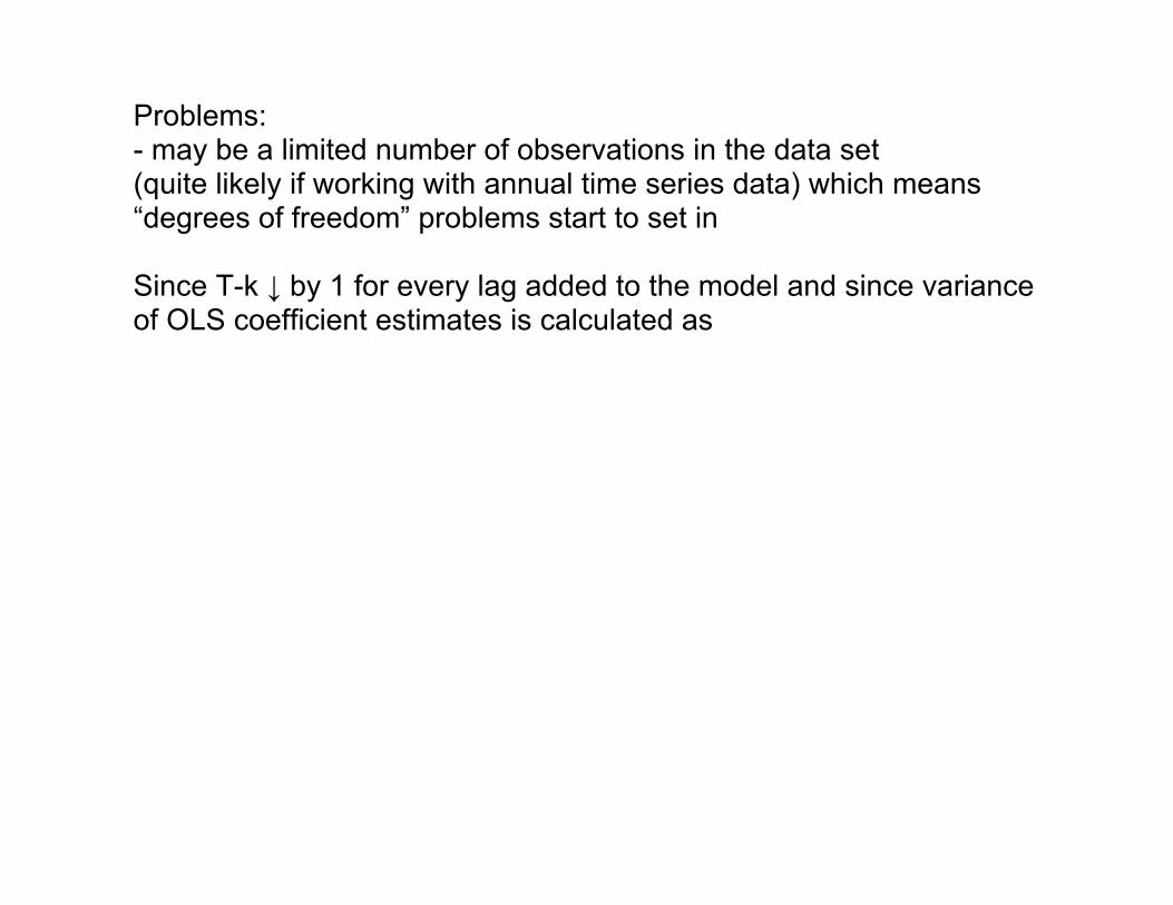
Problems: - may be a limited number of observations in the data set (quite likely if working with annual time series data) which means “degrees of freedom” problems start to set in Since T-k ↓ by 1 for every lag added to the model and since variance of OLS coefficient estimates is calculated as
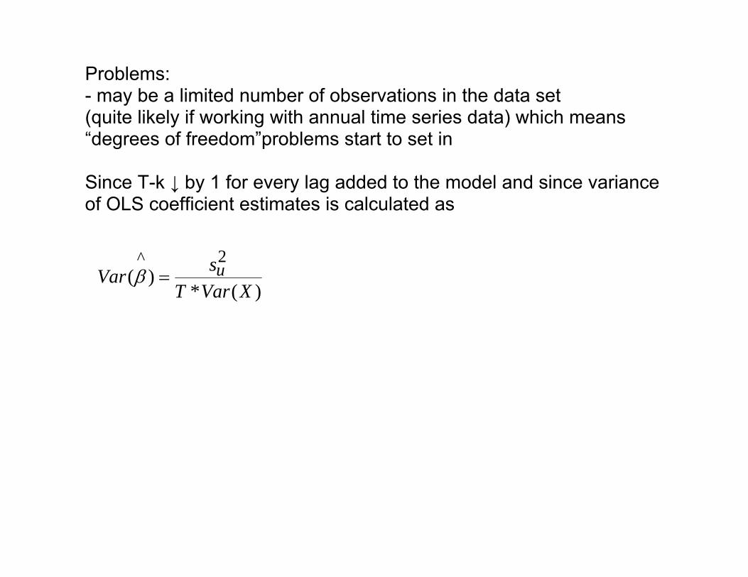
Problems: - may be a limited number of observations in the data set (quite likely if working with annual time series data) which means “degrees of freedom”problems start to set in Since T-k ↓ by 1 for every lag added to the model and since variance of OLS coefficient estimates is calculated as
)(*)(
2^
XVarTsVar u=β
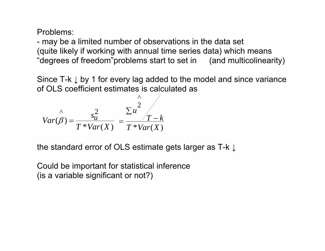
Problems: - may be a limited number of observations in the data set (quite likely if working with annual time series data) which means “degrees of freedom”problems start to set in (and multicolinearity) Since T-k ↓ by 1 for every lag added to the model and since variance of OLS coefficient estimates is calculated as
)(*
^2
XVarTkT
u−
∑=
the standard error of OLS estimate gets larger as T-k ↓ Could be important for statistical inference (is a variable significant or not?)
)(*)(
2^
XVarTsVar u=β
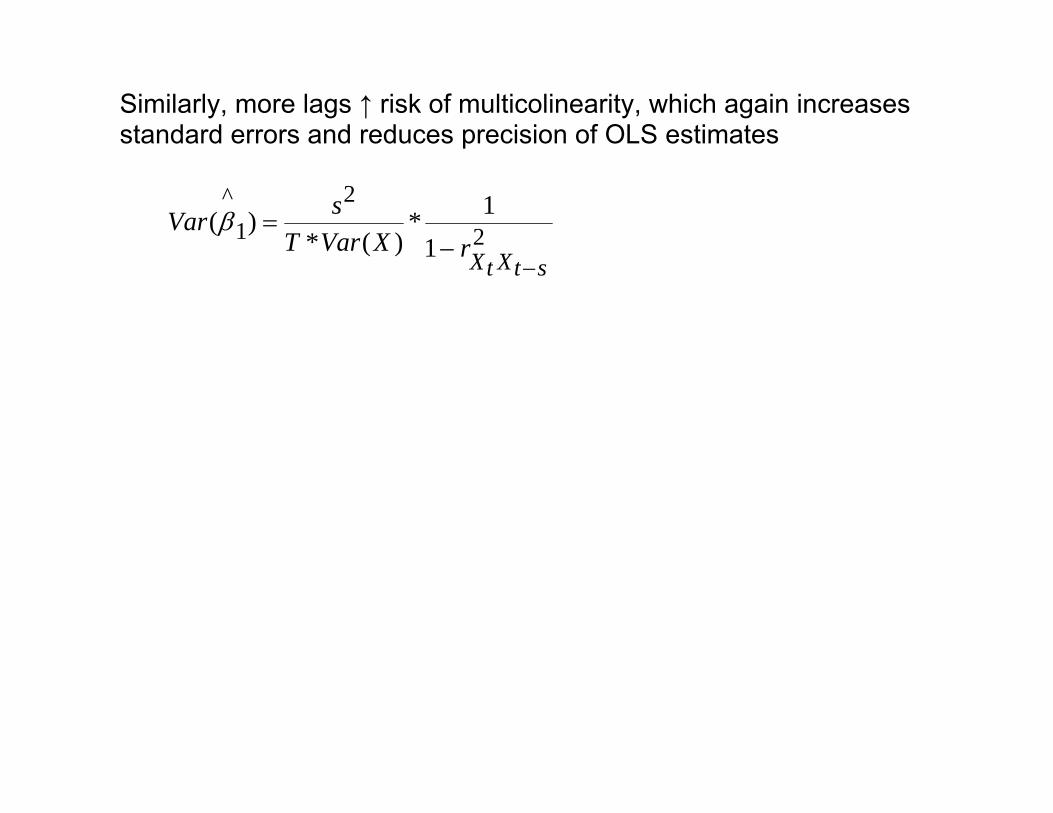
Similarly, more lags ↑ risk of multicolinearity, which again increases standard errors and reduces precision of OLS estimates
2
21
^
11*
)(*)(
stXtXrXVarT
sVar
−−
=β
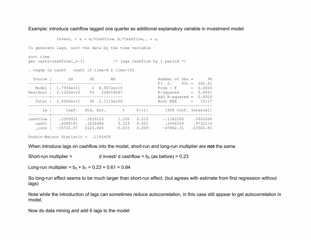
Example: introduce cashflow lagged one quarter as additional explanatory variable in investment model Investt = a + b0*Cashflowt b1*Cashflowt-1 + ut To generate lags, sort the data by the time variable sort time gen cash1=cashflow[_n-1] /* lags cashflow by 1 period */ . regdw ie cashf cash1 if time>8 & time<105 Source | SS df MS Number of obs = 96 ---------+------------------------------ F( 2, 93) = 392.41 Model | 1.7934e+11 2 8.9672e+10 Prob > F = 0.0000 Residual | 2.1252e+10 93 228518067 R-squared = 0.8941 ---------+------------------------------ Adj R-squared = 0.8918 Total | 2.0060e+11 95 2.1115e+09 Root MSE = 15117 ------------------------------------------------------------------------------ ie | Coef. Std. Err. t P>|t| [95% Conf. Interval] ---------+-------------------------------------------------------------------- cashflow | .2309931 .1839125 1.256 0.212 -.1342206 .5962068 cash1 | .6089191 .1834484 3.319 0.001 .2446269 .9732114 _cons | -35721.57 6123.845 -5.833 0.000 -47882.31 -23560.83 Durbin-Watson Statistic = .1145408 When introduce lags on cashflow into the model, short-run and long-run multiplier are not the same
Short-run multiplier = d invest/ d cashflow = b0 (as before) = 0.23 Long-run multiplier = b0 + b1 = 0.23 + 0.61 = 0.84 So long-run effect seems to be much larger than short-run effect, (but agrees with estimate from first regression without lags) Note while the introduction of lags can sometimes reduce autocorrelation, in this case still appear to get autocorrelation in model. Now do data mining and add 6 lags to the model
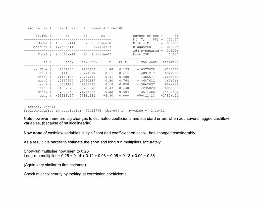
. reg ie cashf cash1-cash6 if time>8 & time<105 Source | SS df MS Number of obs = 96 -------------+------------------------------ F( 7, 88) = 131.17 Model | 1.8305e+11 7 2.6150e+10 Prob > F = 0.0000 Residual | 1.7544e+10 88 199368717 R-squared = 0.9125 -------------+------------------------------ Adj R-squared = 0.9056 Total | 2.0060e+11 95 2.1115e+09 Root MSE = 14120 ------------------------------------------------------------------------------ ie | Coef. Std. Err. t P>|t| [95% Conf. Interval] -------------+---------------------------------------------------------------- cashflow | .2572755 .1786268 1.44 0.153 -.0977078 .6122588 cash1 | .141559 .2771014 0.51 0.611 -.4091217 .6922398 cash2 | .1152186 .2787114 0.41 0.680 -.4386617 .6690988 cash3 | .0837524 .2780237 0.30 0.764 -.4687612 .636266 cash4 | .0501196 .2789373 0.18 0.858 -.5042097 .6044489 cash5 | .1307876 .2789578 0.47 0.640 -.4235823 .6851575 cash6 | .092952 .1783286 0.52 0.604 -.2614386 .4473426 _cons | -39319.27 5783.234 -6.80 0.000 -50812.23 -27826.31 ------------------------------------------------------------------------------ . bgtest, lag(1) Breusch-Godfrey LM statistic: 90.22796 Chi-sq( 1) P-value = 2.1e-21 Note however there are big changes to estimated coefficients and standard errors when add several lagged cashflow variables, (because of multicolinearity) Now none of cashflow variables is significant and coefficient on casht-1 has changed considerably. As a result it is harder to estimate the short and long run multipliers accurately Short-run multiplier now risen to 0.26 Long-run multiplier = 0.25 + 0.14 + 0.12 + 0.08 + 0.05 + 0.13 + 0.09 = 0.86 (Again very similar to first estimate) Check multicolinearity by looking at correlation coefficients.
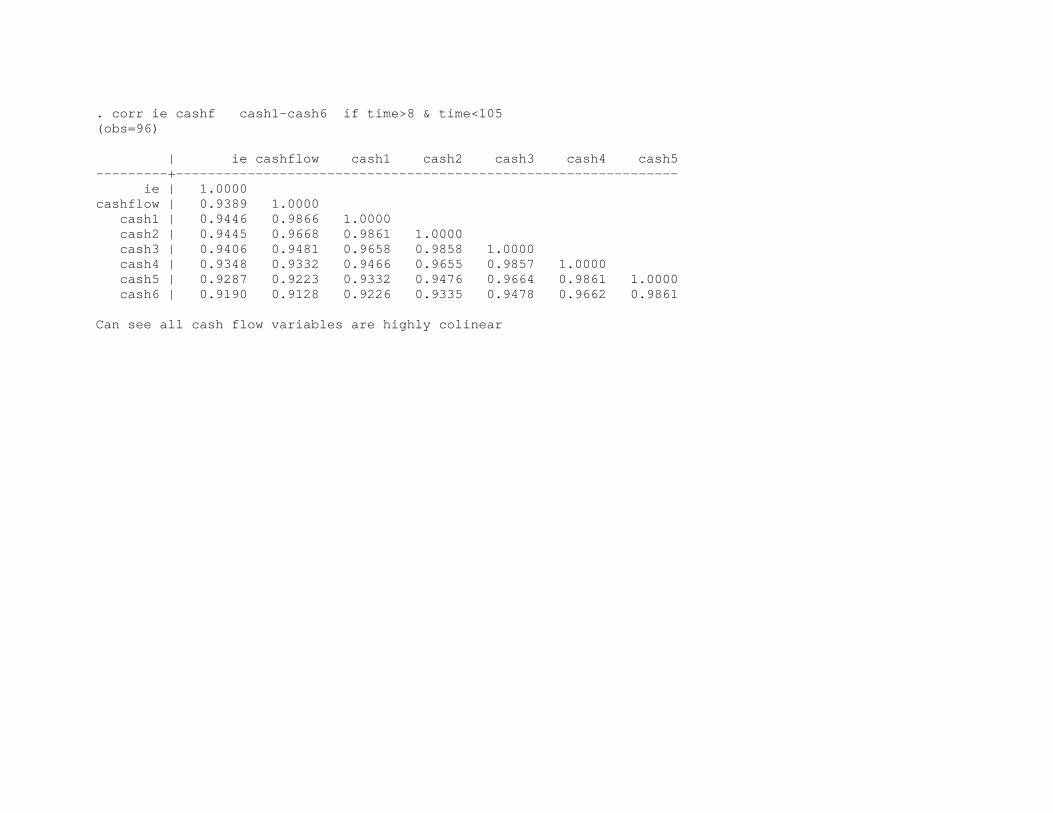
. corr ie cashf cash1-cash6 if time>8 & time<105 (obs=96) | ie cashflow cash1 cash2 cash3 cash4 cash5 ---------+--------------------------------------------------------------- ie | 1.0000 cashflow | 0.9389 1.0000 cash1 | 0.9446 0.9866 1.0000 cash2 | 0.9445 0.9668 0.9861 1.0000 cash3 | 0.9406 0.9481 0.9658 0.9858 1.0000 cash4 | 0.9348 0.9332 0.9466 0.9655 0.9857 1.0000 cash5 | 0.9287 0.9223 0.9332 0.9476 0.9664 0.9861 1.0000 cash6 | 0.9190 0.9128 0.9226 0.9335 0.9478 0.9662 0.9861 Can see all cash flow variables are highly colinear
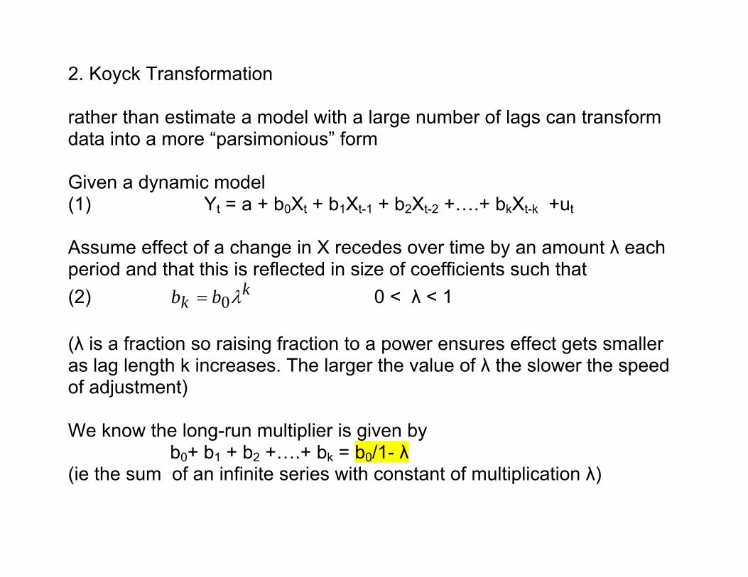
2. Koyck Transformation rather than estimate a model with a large number of lags can transform data into a more “parsimonious” form Given a dynamic model (1) Yt = a + b0Xt + b1Xt-1 + b2Xt-2 +….+ bkXt-k +ut Assume effect of a change in X recedes over time by an amount λ each period and that this is reflected in size of coefficients such that (2) k
k bb λ0= 0 < λ < 1 (λ is a fraction so raising fraction to a power ensures effect gets smaller as lag length k increases. The larger the value of λ the slower the speed of adjustment) We know the long-run multiplier is given by b0+ b1 + b2 +….+ bk = b0/1- λ (ie the sum of an infinite series with constant of multiplication λ)
Sub. (2) into (1) (3) Yt = a + b0Xt + b0λ Xt-1 + b2λ2 Xt-2 +….+ bk λkXt-k +ut If (3) is true at time t it is also true at time t-1, so (4) Yt-1 = a + b0Xt-1 + b0λ Xt-2 + b0λ2 Xt-3 +….+ b0 λkXt-k-1 +ut
multiply (4) by λ (5) λYt-1 = λa + b0λXt-1 + b0λ2Xt-2 + b0λ3 Xt-3 +… b0 λk+1Xt-k-1 + λ ut (3) – (5)
Yt - λYt-1 = a - λa + b0Xt + ut- λ ut (6) Yt = (a – λa) + b0Xt + λYt-1 + vt (where vt = ut- λ ut) ie regress Yt on a constant, the current level of X and the value of Y lagged 1 period. The coefficients b0 and λ are what you need to calculate the long run multiplier
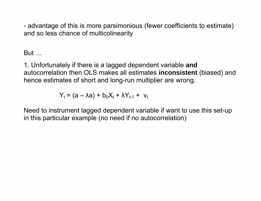
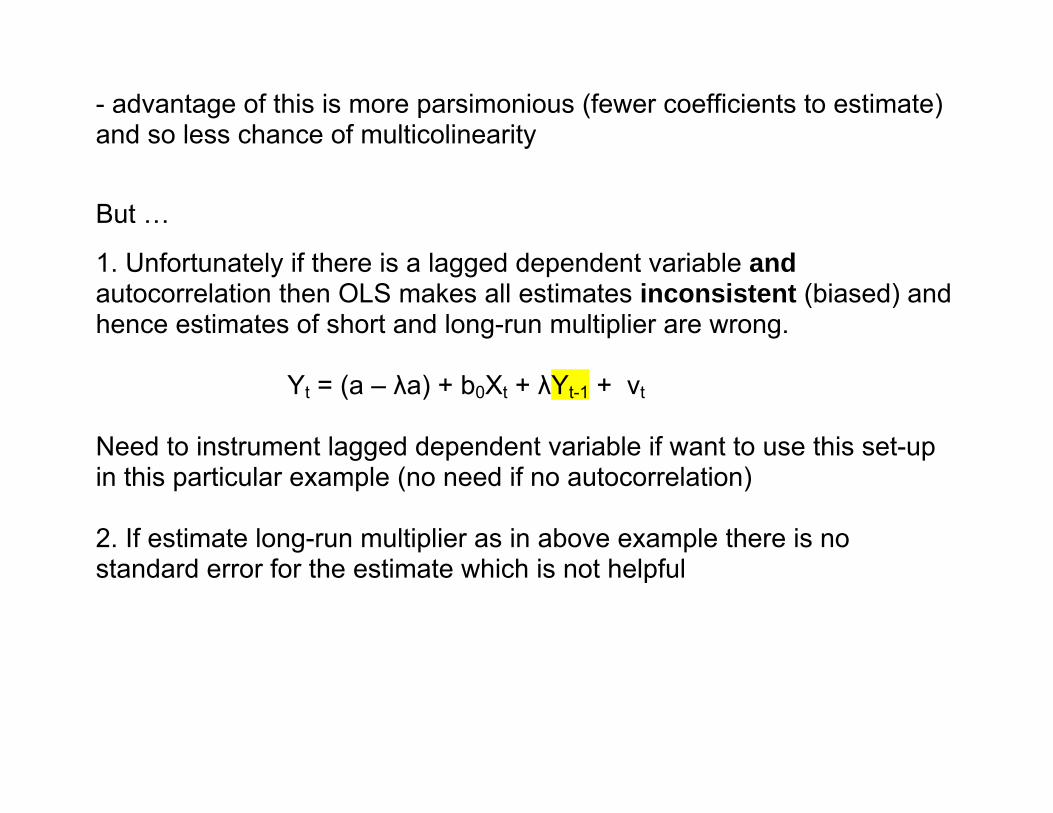
- advantage of this is more parsimonious (fewer coefficients to estimate) and so less chance of multicolinearity
- advantage of this is more parsimonious (fewer coefficients to estimate) and so less chance of multicolinearity
But …
- advantage of this is more parsimonious (fewer coefficients to estimate) and so less chance of multicolinearity
But …
1. Unfortunately if there is a lagged dependent variable and autocorrelation then OLS makes all estimates inconsistent (biased) and hence estimates of short and long-run multiplier are wrong.
Yt = (a – λa) + b0Xt + λYt-1 + vt
- advantage of this is more parsimonious (fewer coefficients to estimate) and so less chance of multicolinearity
But …
1. Unfortunately if there is a lagged dependent variable and autocorrelation then OLS makes all estimates inconsistent (biased) and hence estimates of short and long-run multiplier are wrong.
Yt = (a – λa) + b0Xt + λYt-1 + vt Need to instrument lagged dependent variable if want to use this set-up in this particular example (no need if no autocorrelation)
- advantage of this is more parsimonious (fewer coefficients to estimate) and so less chance of multicolinearity
But …
1. Unfortunately if there is a lagged dependent variable and autocorrelation then OLS makes all estimates inconsistent (biased) and hence estimates of short and long-run multiplier are wrong.
Yt = (a – λa) + b0Xt + λYt-1 + vt
Need to instrument lagged dependent variable if want to use this set-up in this particular example (no need if no autocorrelation) 2. If estimate long-run multiplier as in above example there is no standard error for the estimate which is not helpful
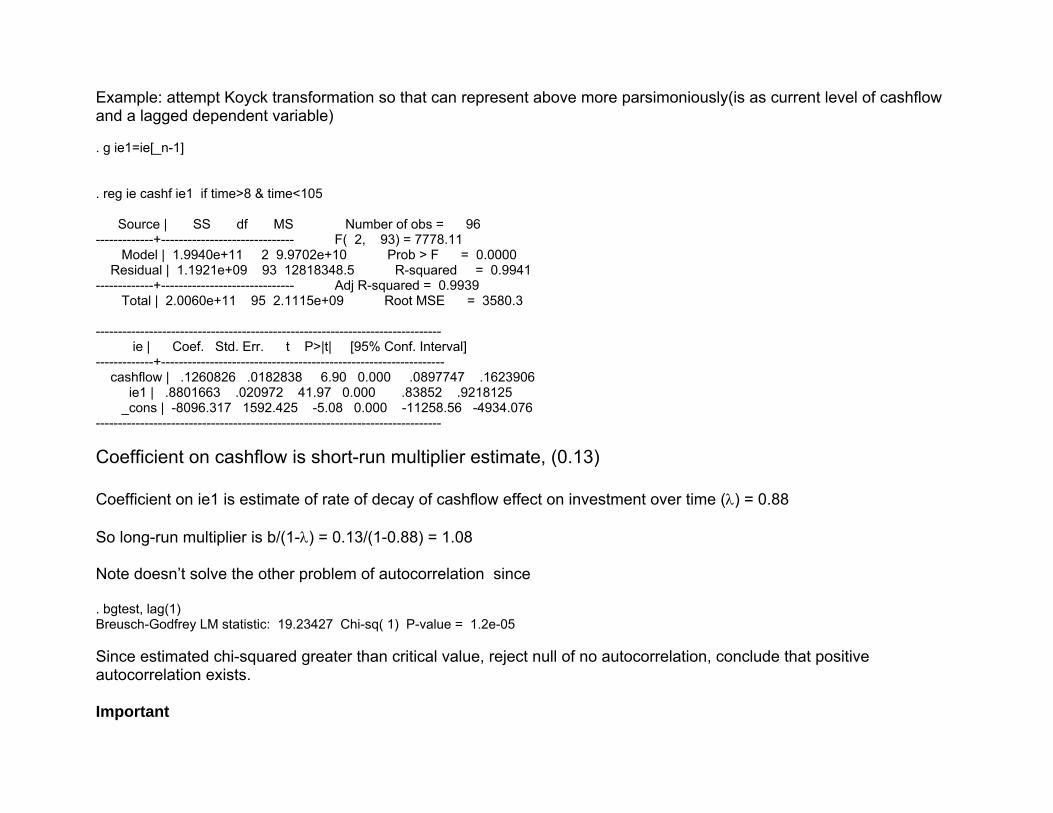
Example: attempt Koyck transformation so that can represent above more parsimoniously(is as current level of cashflow and a lagged dependent variable) . g ie1=ie[_n-1] . reg ie cashf ie1 if time>8 & time<105 Source | SS df MS Number of obs = 96 -------------+------------------------------ F( 2, 93) = 7778.11 Model | 1.9940e+11 2 9.9702e+10 Prob > F = 0.0000 Residual | 1.1921e+09 93 12818348.5 R-squared = 0.9941 -------------+------------------------------ Adj R-squared = 0.9939 Total | 2.0060e+11 95 2.1115e+09 Root MSE = 3580.3 ------------------------------------------------------------------------------ ie | Coef. Std. Err. t P>|t| [95% Conf. Interval] -------------+---------------------------------------------------------------- cashflow | .1260826 .0182838 6.90 0.000 .0897747 .1623906 ie1 | .8801663 .020972 41.97 0.000 .83852 .9218125 _cons | -8096.317 1592.425 -5.08 0.000 -11258.56 -4934.076 ------------------------------------------------------------------------------ Coefficient on cashflow is short-run multiplier estimate, (0.13) Coefficient on ie1 is estimate of rate of decay of cashflow effect on investment over time (λ) = 0.88 So long-run multiplier is b/(1-λ) = 0.13/(1-0.88) = 1.08 Note doesn’t solve the other problem of autocorrelation since
. bgtest, lag(1) Breusch-Godfrey LM statistic: 19.23427 Chi-sq( 1) P-value = 1.2e-05 Since estimated chi-squared greater than critical value, reject null of no autocorrelation, conclude that positive autocorrelation exists. Important
To get round this, can also show that can estimate long run multiplier and its standard error directly from the specification
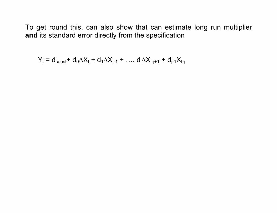
To get round this, can also show that can estimate long run multiplier and its standard error directly from the specification Yt = dconst+ d0ΔXt + d1ΔXt-1 + …. djΔXt-j+1 + dj-1Xt-j
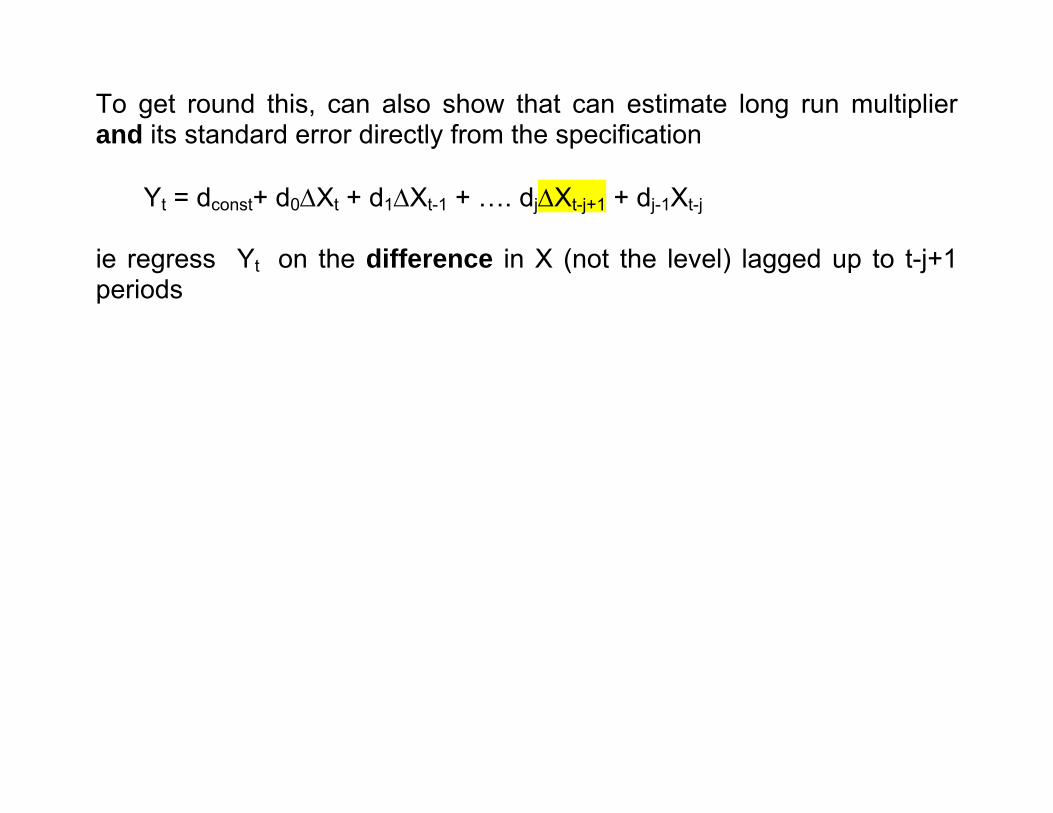
To get round this, can also show that can estimate long run multiplier and its standard error directly from the specification Yt = dconst+ d0ΔXt + d1ΔXt-1 + …. djΔXt-j+1 + dj-1Xt-j ie regress Yt on the difference in X (not the level) lagged up to t-j+1 periods
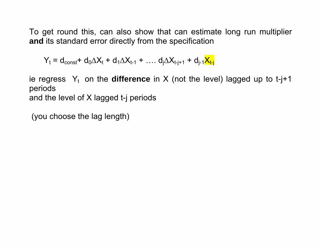
To get round this, can also show that can estimate long run multiplier and its standard error directly from the specification Yt = dconst+ d0ΔXt + d1ΔXt-1 + …. djΔXt-j+1 + dj-1Xt-j ie regress Yt on the difference in X (not the level) lagged up to t-j+1 periods and the level of X lagged t-j periods (you choose the lag length)
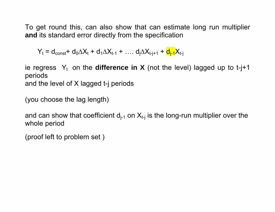
To get round this, can also show that can estimate long run multiplier and its standard error directly from the specification Yt = dconst+ d0ΔXt + d1ΔXt-1 + …. djΔXt-j+1 + dj-1Xt-j ie regress Yt on the difference in X (not the level) lagged up to t-j+1 periods and the level of X lagged t-j periods (you choose the lag length) and can show that coefficient dj-1 on Xt-j is the long-run multiplier over the whole period (proof left to problem set )
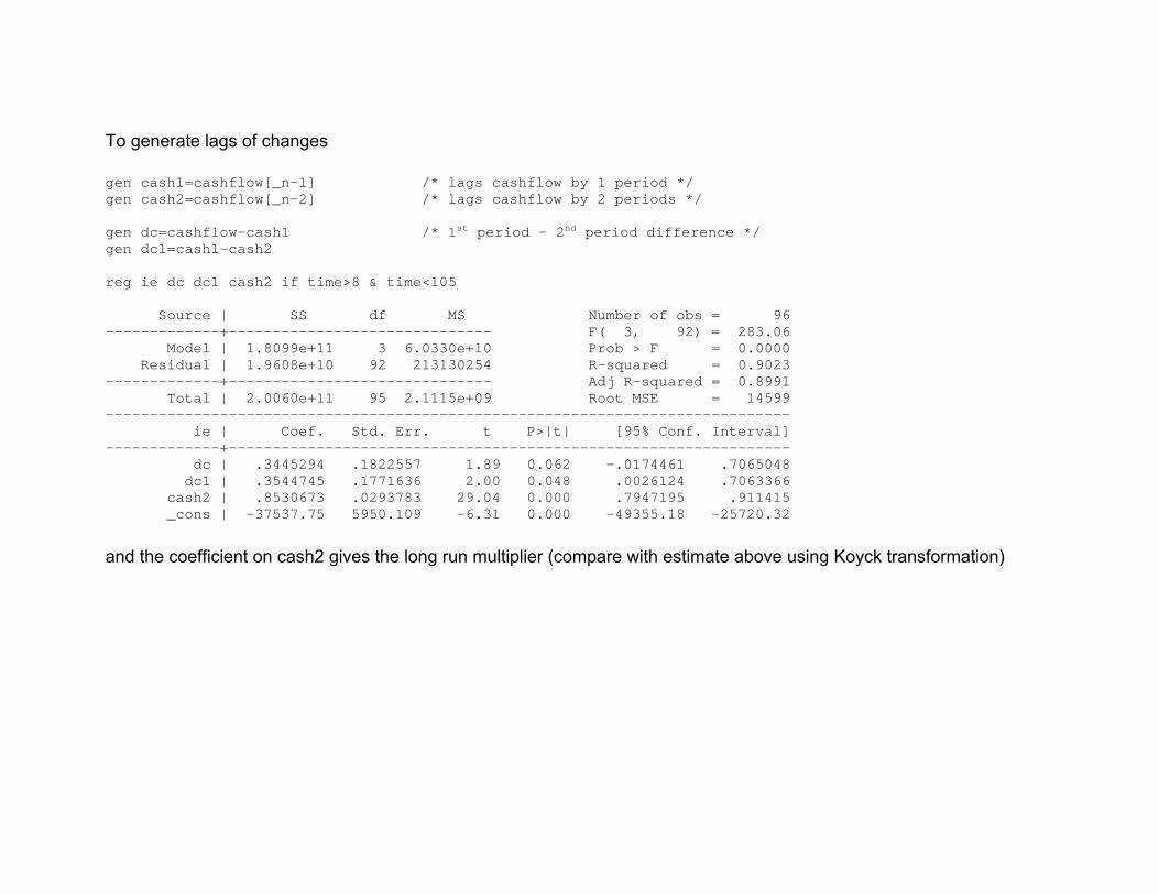
To generate lags of changes gen cash1=cashflow[_n-1] /* lags cashflow by 1 period */ gen cash2=cashflow[_n-2] /* lags cashflow by 2 periods */ gen dc=cashflow-cash1 /* 1st period – 2nd period difference */ gen dc1=cash1-cash2 reg ie dc dc1 cash2 if time>8 & time<105 Source | SS df MS Number of obs = 96 -------------+------------------------------ F( 3, 92) = 283.06 Model | 1.8099e+11 3 6.0330e+10 Prob > F = 0.0000 Residual | 1.9608e+10 92 213130254 R-squared = 0.9023 -------------+------------------------------ Adj R-squared = 0.8991 Total | 2.0060e+11 95 2.1115e+09 Root MSE = 14599 ------------------------------------------------------------------------------ ie | Coef. Std. Err. t P>|t| [95% Conf. Interval] -------------+---------------------------------------------------------------- dc | .3445294 .1822557 1.89 0.062 -.0174461 .7065048 dc1 | .3544745 .1771636 2.00 0.048 .0026124 .7063366 cash2 | .8530673 .0293783 29.04 0.000 .7947195 .911415 _cons | -37537.75 5950.109 -6.31 0.000 -49355.18 -25720.32
and the coefficient on cash2 gives the long run multiplier (compare with estimate above using Koyck transformation)
Stationarity Ultimately whether you can sensibly include lags of either the dependent or explanatory variables or indeed the current level of a variable in a regression also depends on whether the time series data that you are analysing are stationary
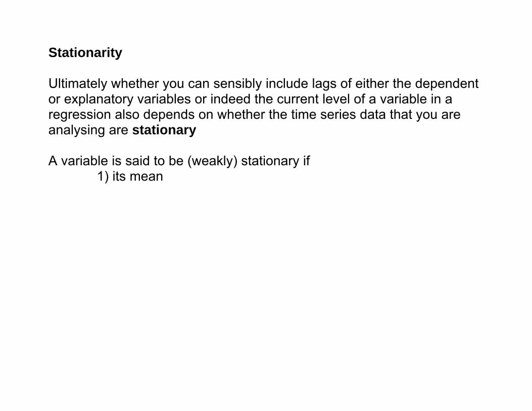
Stationarity Ultimately whether you can sensibly include lags of either the dependent or explanatory variables or indeed the current level of a variable in a regression also depends on whether the time series data that you are analysing are stationary A variable is said to be (weakly) stationary if
1) its mean
Stationarity Ultimately whether you can sensibly include lags of either the dependent or explanatory variables or indeed the current level of a variable in a regression also depends on whether the time series data that you are analysing are stationary A variable is said to be (weakly) stationary if
1) its mean 2) its variance
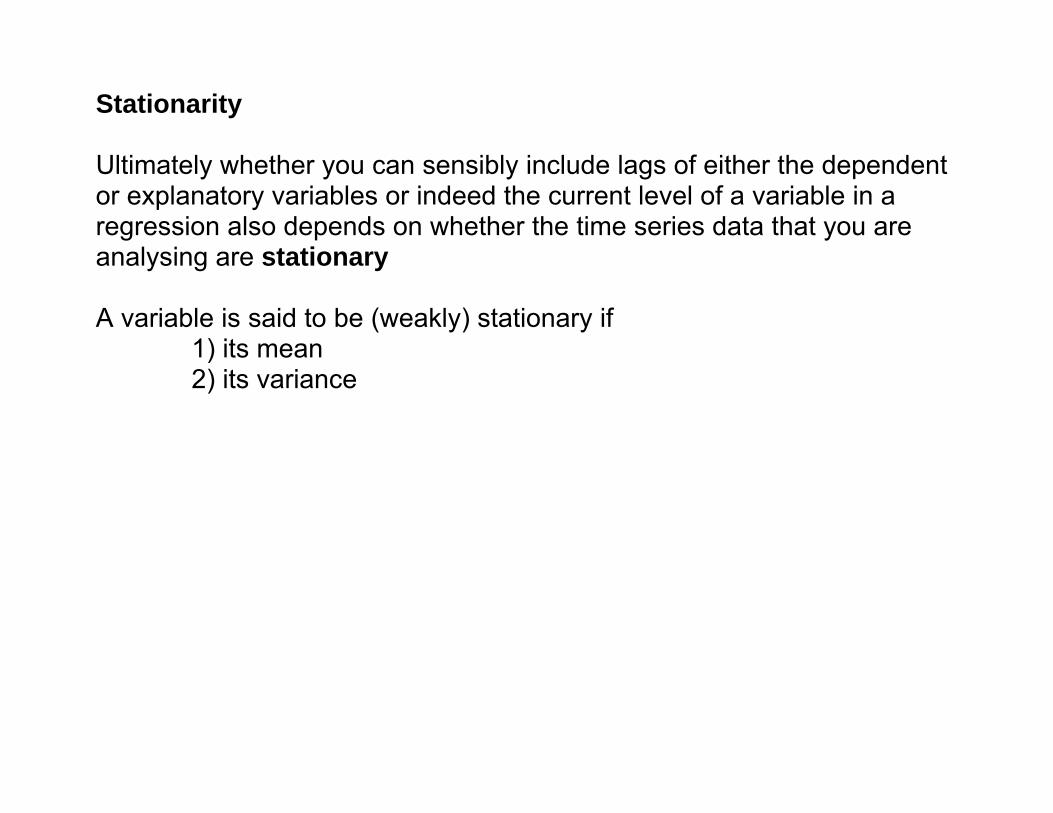
Stationarity Ultimately whether you can sensibly include lags of either the dependent or explanatory variables or indeed the current level of a variable in a regression also depends on whether the time series data that you are analysing are stationary A variable is said to be (weakly) stationary if
1) its mean 2) its variance 3) its autocovariance Cov(Yt, Yt-s) where s ≠ t
do not change over time
Stationarity Ultimately whether you can sensibly include lags of either the dependent or explanatory variables or indeed the current level of a variable in a regression also depends on whether the time series data that you are analysing are stationary A variable is said to be (weakly) stationary if
1) its mean 2) its variance 3) its autocovariance Cov(Yt, Yt-s) where s ≠ t
do not change over time Stationarity is needed if the Gauss-Markov conditions for unbiased, efficient OLS estimation are to be met by time series data
Stationarity Ultimately whether you can sensibly include lags of either the dependent or explanatory variables or indeed the current level of a variable in a regression also depends on whether the time series data that you are analysing are stationary A variable is said to be (weakly) stationary if
1) its mean 2) its variance 3) its autocovariance Cov(Yt, Yt-s) where s ≠ t
do not change over time Stationarity is needed if the Gauss-Markov conditions for unbiased, efficient OLS estimation are to be met by time series data (Essentially any variable that is trended is unlikely to be stationary)
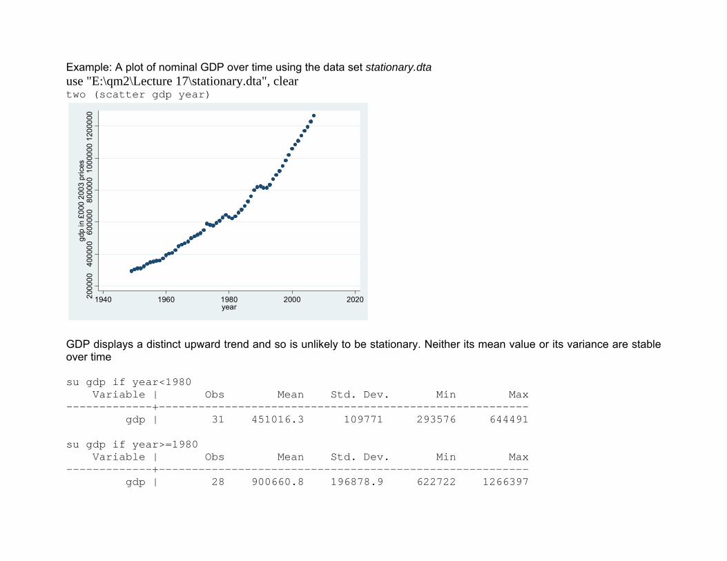
Example: A plot of nominal GDP over time using the data set stationary.dta use "E:\qm2\Lecture 17\stationary.dta", clear two (scatter gdp year)
2000
0040
0000
6000
0080
0000
1000
000
1200
000
gdp
in £
000
2003
pric
es
1940 1960 1980 2000 2020year
GDP displays a distinct upward trend and so is unlikely to be stationary. Neither its mean value or its variance are stable over time su gdp if year<1980 Variable | Obs Mean Std. Dev. Min Max -------------+-------------------------------------------------------- gdp | 31 451016.3 109771 293576 644491 su gdp if year>=1980 Variable | Obs Mean Std. Dev. Min Max -------------+-------------------------------------------------------- gdp | 28 900660.8 196878.9 622722 1266397
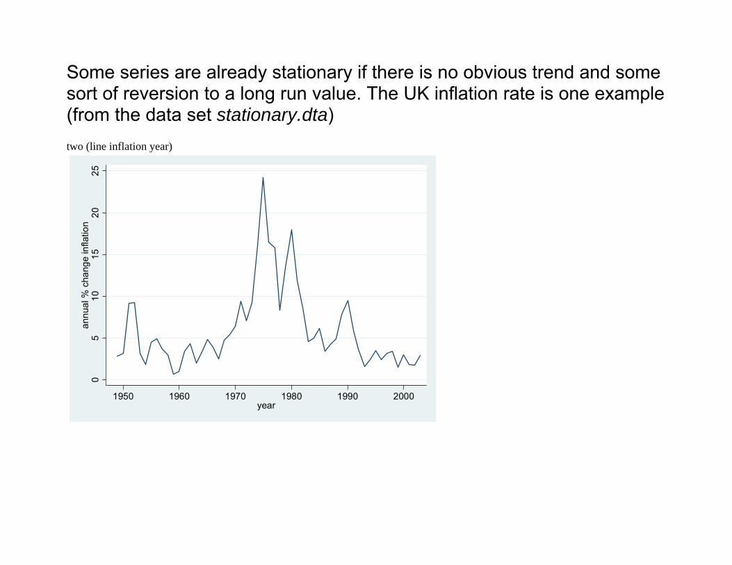
Some series are already stationary if there is no obvious trend and some sort of reversion to a long run value. The UK inflation rate is one example (from the data set stationary.dta) two (line inflation year)
05
1015
2025
annu
al %
cha
nge
infla
tion
1950 1960 1970 1980 1990 2000year

In general just looking at the time series of a variable will not be enough to judge whether the variable is stationary or not (though it is good practice to graph the series anyway)
In general just looking at the time series of a variable will not be enough to judge whether the variable is stationary or not (though it is good practice to graph the series anyway) If a variable is stationary then its values are persistent. This means that the level of the variable at some point in the past continues to influence the level of the variable today.
In general just looking at the time series of a variable will not be enough to judge whether the variable is stationary or not (though it is good practice to graph the series anyway) If a variable is stationary then its values are persistent. This means that the level of the variable at some point in the past continues to influence the level of the variable today. The simplest way of modelling persistence of a non-stationary process is the random walk
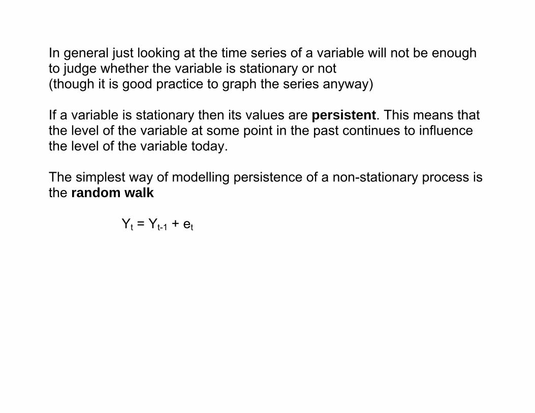
In general just looking at the time series of a variable will not be enough to judge whether the variable is stationary or not (though it is good practice to graph the series anyway) If a variable is stationary then its values are persistent. This means that the level of the variable at some point in the past continues to influence the level of the variable today. The simplest way of modelling persistence of a non-stationary process is the random walk
Yt = Yt-1 + et
- the value of Y today equals last period’s value plus an unpredictable random error e (hence the name) and no other lags
In general just looking at the time series of a variable will not be enough to judge whether the variable is stationary or not (though it is good practice to graph the series anyway) If a variable is stationary then its values are persistent. This means that the level of the variable at some point in the past continues to influence the level of the variable today. The simplest way of modelling persistence of a non-stationary process is the random walk
Yt = Yt-1 + et
- the value of Y today equals last period’s value plus an unpredictable random error e (hence the name) and no other lags This means that the best forecast of this period’s level is last period’s level.
Yt = Yt-1 + et
Yt = ρYt-1 + et similar then to the AR(1) model used for autocorrelation but with the coefficient ρ set to “1”
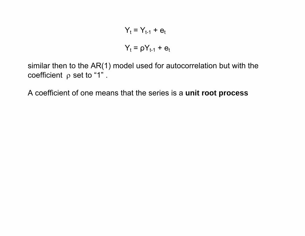
Yt = Yt-1 + et
Yt = ρYt-1 + et similar then to the AR(1) model used for autocorrelation but with the coefficient ρ set to “1” . A coefficient of one means that the series is a unit root process

Yt = Yt-1 + et
Yt = ρYt-1 + et similar then to the AR(1) model used for autocorrelation but with the coefficient ρ set to “1” . A coefficient of one means that the series is a unit root process
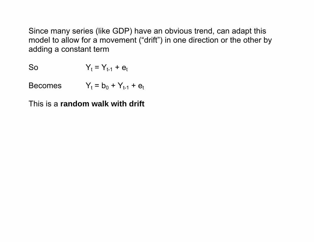
Since many series (like GDP) have an obvious trend, can adapt this model to allow for a movement (“drift”) in one direction or the other by adding a constant term
Since many series (like GDP) have an obvious trend, can adapt this model to allow for a movement (“drift”) in one direction or the other by adding a constant term So Yt = Yt-1 + et
Since many series (like GDP) have an obvious trend, can adapt this model to allow for a movement (“drift”) in one direction or the other by adding a constant term So Yt = Yt-1 + et Becomes Yt = b0 + Yt-1 + et
Since many series (like GDP) have an obvious trend, can adapt this model to allow for a movement (“drift”) in one direction or the other by adding a constant term So Yt = Yt-1 + et Becomes Yt = b0 + Yt-1 + et
This is a random walk with drift
Since many series (like GDP) have an obvious trend, can adapt this model to allow for a movement (“drift”) in one direction or the other by adding a constant term So Yt = Yt-1 + et Becomes Yt = b0 + Yt-1 + et
This is a random walk with drift the best forecast of this period’s level is now is last period’s value plus a positive constant b0 (more realistic model of GDP growing at say 2% a year)
Since many series (like GDP) have an obvious trend, can adapt this model to allow for a movement (“drift”) in one direction or the other by adding a constant term So Yt = Yt-1 + et Becomes Yt = b0 + Yt-1 + et
This is a random walk with drift the best forecast of this period’s level is now is last period’s value plus a positive constant b0 (more realistic model of GDP growing at say 2% a year) Can also model this by adding a time trend (t=year)
Yt = b0 + Yt-1 + t + et
Since many series (like GDP) have an obvious trend, can adapt this model to allow for a movement (“drift”) in one direction or the other by adding a constant term So Yt = Yt-1 + et Becomes Yt = b0 + Yt-1 + et
This is a random walk with drift the best forecast of this period’s level is now is last period’s value plus a positive constant b0 (more realistic model of GDP growing at say 2% a year) Can also model this by adding a time trend (t=year)
Yt = b0 + Yt-1 + t + et – what this means is that a series can be stationary around an upward (or downward) trend
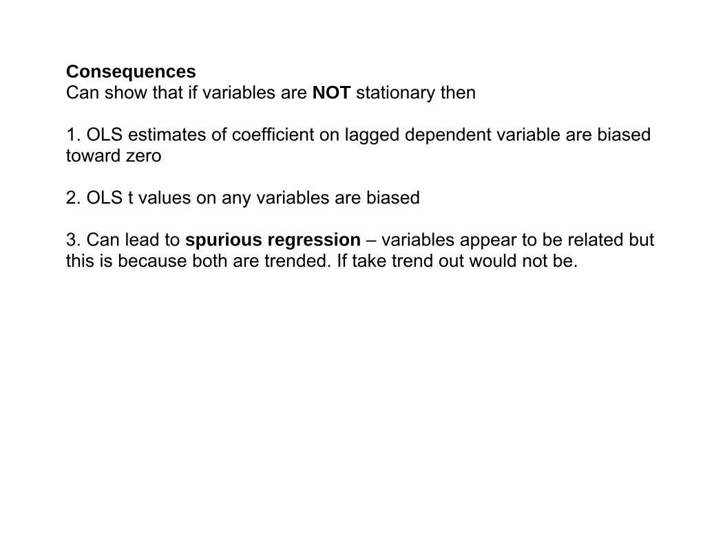
Consequences Can show that if variables are NOT stationary then
Consequences Can show that if variables are NOT stationary then 1. OLS estimates of coefficient on lagged dependent variable are biased toward zero
Consequences Can show that if variables are NOT stationary then 1. OLS estimates of coefficient on lagged dependent variable are biased toward zero 2. OLS t values on any variables are biased

Consequences Can show that if variables are NOT stationary then 1. OLS estimates of coefficient on lagged dependent variable are biased toward zero 2. OLS t values on any variables are biased 3. Can lead to spurious regression – variables appear to be related but this is because both are trended. If take trend out would not be.
Consequences Can show that if variables are NOT stationary then 1. OLS estimates of coefficient on lagged dependent variable are biased toward zero 2. OLS t values on any variables are biased 3. Can lead to spurious regression – variables appear to be related but this is because both are trended. If take trend out would not be. (4. Durbin Watson values are biased down (toward 0) )
Note that any concerns about endogeneity are dwarfed compared to the issue of stationarity since the bias in OLS is given by
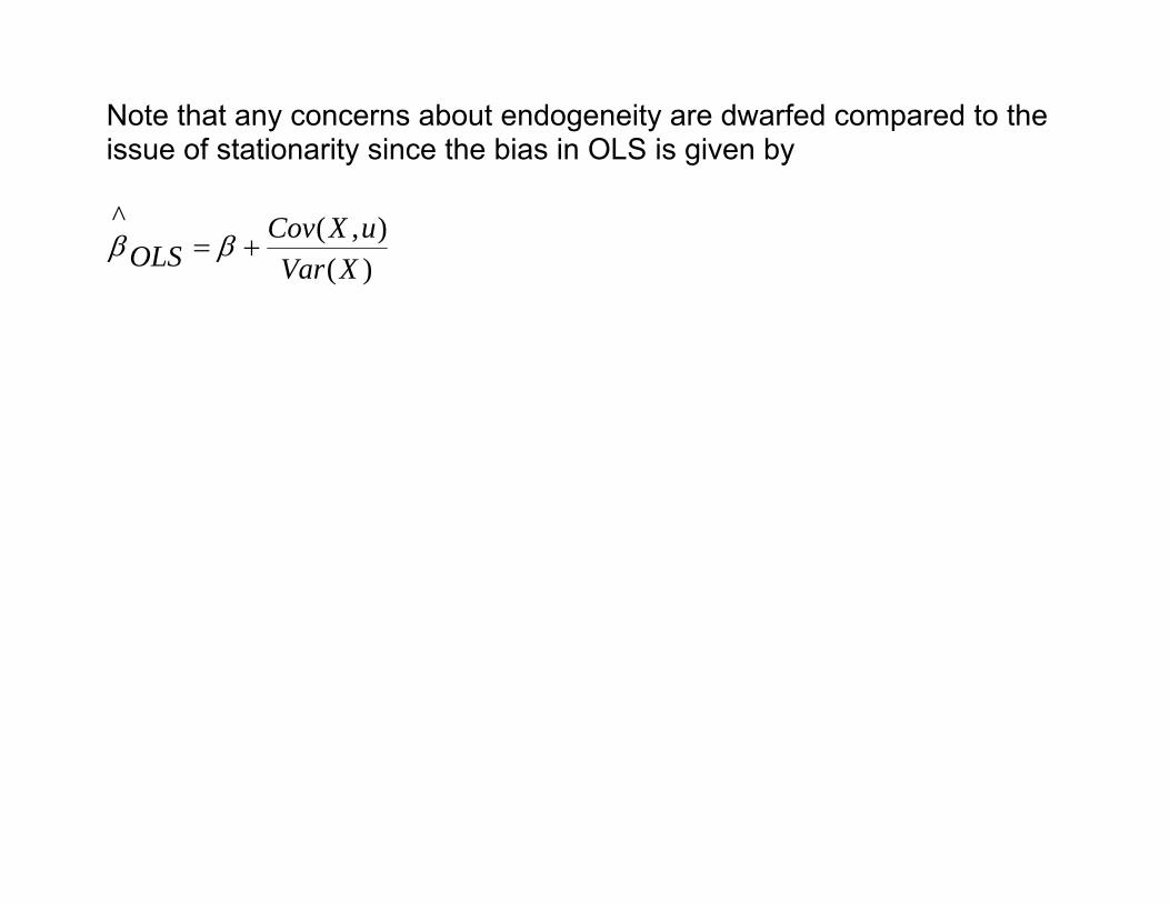
Note that any concerns about endogeneity are dwarfed compared to the issue of stationarity since the bias in OLS is given by
)(),(^
XVaruXCov
OLS += ββ
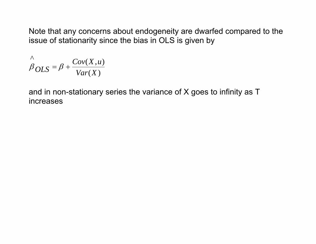
Note that any concerns about endogeneity are dwarfed compared to the issue of stationarity since the bias in OLS is given by
)(),(^
XVaruXCov
OLS += ββ
and in non-stationary series the variance of X goes to infinity as T increases
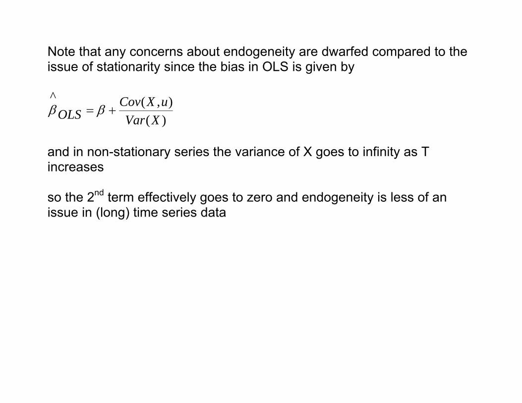
Note that any concerns about endogeneity are dwarfed compared to the issue of stationarity since the bias in OLS is given by
)(),(^
XVaruXCov
OLS += ββ
and in non-stationary series the variance of X goes to infinity as T increases so the 2nd term effectively goes to zero and endogeneity is less of an issue in (long) time series data
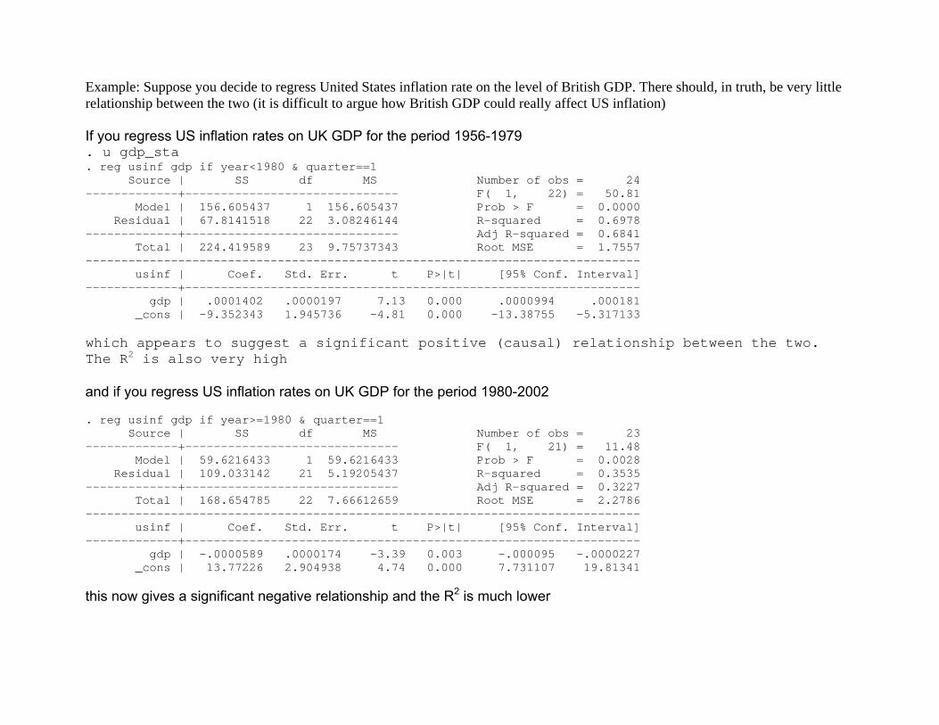
Example: Suppose you decide to regress United States inflation rate on the level of British GDP. There should, in truth, be very little relationship between the two (it is difficult to argue how British GDP could really affect US inflation) If you regress US inflation rates on UK GDP for the period 1956-1979 . u gdp_sta . reg usinf gdp if year<1980 & quarter==1 Source | SS df MS Number of obs = 24 -------------+------------------------------ F( 1, 22) = 50.81 Model | 156.605437 1 156.605437 Prob > F = 0.0000 Residual | 67.8141518 22 3.08246144 R-squared = 0.6978 -------------+------------------------------ Adj R-squared = 0.6841 Total | 224.419589 23 9.75737343 Root MSE = 1.7557 ------------------------------------------------------------------------------ usinf | Coef. Std. Err. t P>|t| [95% Conf. Interval] -------------+---------------------------------------------------------------- gdp | .0001402 .0000197 7.13 0.000 .0000994 .000181 _cons | -9.352343 1.945736 -4.81 0.000 -13.38755 -5.317133 which appears to suggest a significant positive (causal) relationship between the two. The R2 is also very high and if you regress US inflation rates on UK GDP for the period 1980-2002 . reg usinf gdp if year>=1980 & quarter==1 Source | SS df MS Number of obs = 23 -------------+------------------------------ F( 1, 21) = 11.48 Model | 59.6216433 1 59.6216433 Prob > F = 0.0028 Residual | 109.033142 21 5.19205437 R-squared = 0.3535 -------------+------------------------------ Adj R-squared = 0.3227 Total | 168.654785 22 7.66612659 Root MSE = 2.2786 ------------------------------------------------------------------------------ usinf | Coef. Std. Err. t P>|t| [95% Conf. Interval] -------------+---------------------------------------------------------------- gdp | -.0000589 .0000174 -3.39 0.003 -.000095 -.0000227 _cons | 13.77226 2.904938 4.74 0.000 7.731107 19.81341 this now gives a significant negative relationship and the R2 is much lower
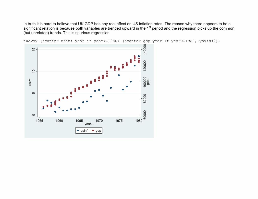
In truth it is hard to believe that UK GDP has any real effect on US inflation rates. The reason why there appears to be a significant relation is because both variables are trended upward in the 1st period and the regression picks up the common (but unrelated) trends. This is spurious regression twoway (scatter usinf year if year<=1980) (scatter gdp year if year<=1980, yaxis(2))
6000
080
000
1000
0012
0000
1400
00gd
p
05
1015
usin
f
1955 1960 1965 1970 1975 1980year...
usinf gdp
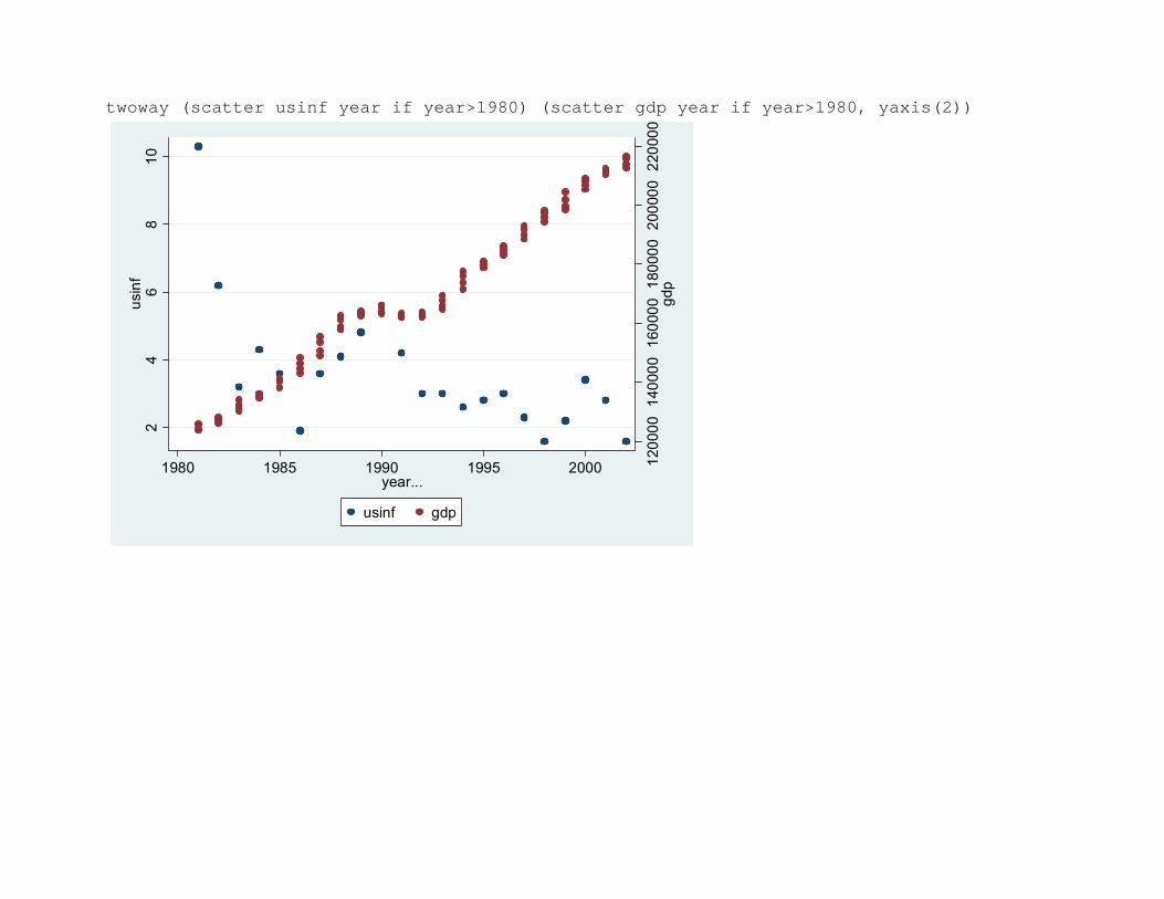
twoway (scatter usinf year if year>1980) (scatter gdp year if year>1980, yaxis(2))
1200
0014
0000
1600
0018
0000
2000
0022
0000
gdp
24
68
10us
inf
1980 1985 1990 1995 2000year...
usinf gdp

Stationarity Ultimately whether you can sensibly include lags of either the dependent or explanatory variables or indeed the current level of a variable in a regression also depends on whether the time series data that you are analysing are stationary A variable is said to be (weakly) stationary if
1) its mean 2) its variance 3) its autocovariance Cov(Yt, Yt-s) where s ≠ t
do not change over time Stationarity is needed if the Gauss-Markov conditions for unbiased, efficient OLS estimation are to be met by time series data (Essentially any variable that is trended is unlikely to be stationary)
Consequences Can show that if variables are NOT stationary then 1. OLS estimates of coefficient on lagged dependent variable are biased toward zero 2. OLS t values on any variables are biased 3. Can lead to spurious regression – variables appear to be related but this is because both are trended. If take trend out would not be.

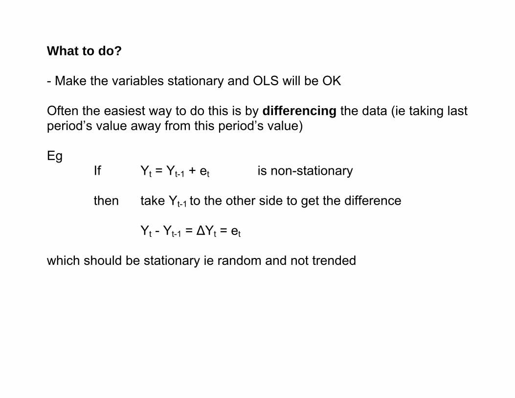
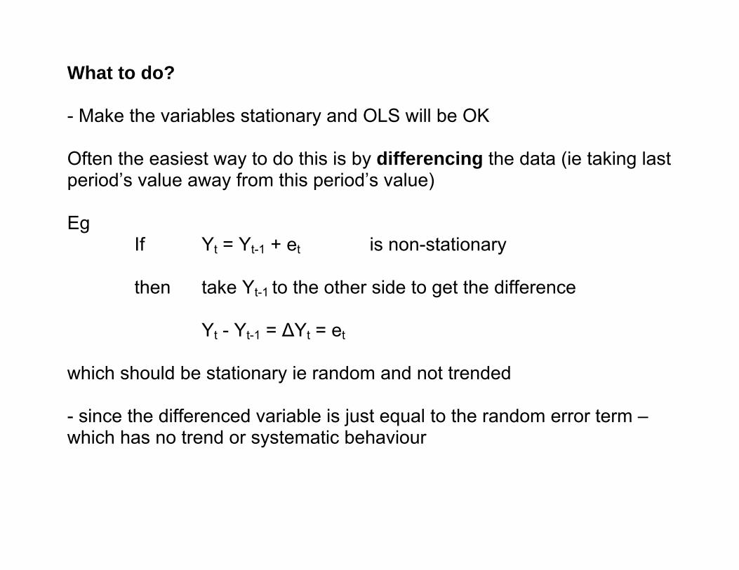
What to do?

What to do? - Make the variables stationary and OLS will be OK
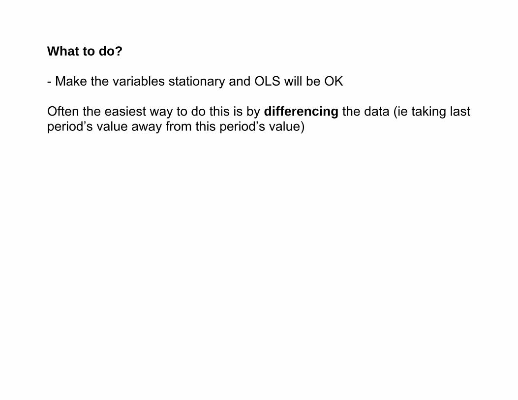
What to do? - Make the variables stationary and OLS will be OK Often the easiest way to do this is by differencing the data (ie taking last period’s value away from this period’s value)
What to do? - Make the variables stationary and OLS will be OK Often the easiest way to do this is by differencing the data (ie taking last period’s value away from this period’s value) Eg
If Yt = Yt-1 + et is non-stationary
What to do? - Make the variables stationary and OLS will be OK Often the easiest way to do this is by differencing the data (ie taking last period’s value away from this period’s value) Eg
If Yt = Yt-1 + et is non-stationary then take Yt-1 to the other side to get the difference
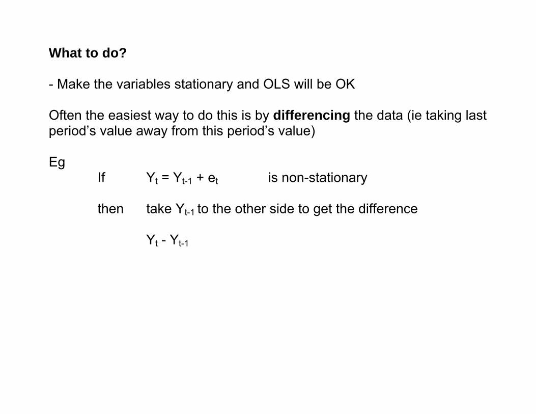
What to do? - Make the variables stationary and OLS will be OK Often the easiest way to do this is by differencing the data (ie taking last period’s value away from this period’s value) Eg
If Yt = Yt-1 + et is non-stationary then take Yt-1 to the other side to get the difference
Yt - Yt-1
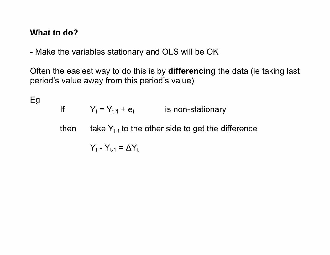
What to do? - Make the variables stationary and OLS will be OK Often the easiest way to do this is by differencing the data (ie taking last period’s value away from this period’s value) Eg
If Yt = Yt-1 + et is non-stationary then take Yt-1 to the other side to get the difference
Yt - Yt-1 = ΔYt
What to do? - Make the variables stationary and OLS will be OK Often the easiest way to do this is by differencing the data (ie taking last period’s value away from this period’s value) Eg
If Yt = Yt-1 + et is non-stationary then take Yt-1 to the other side to get the difference
Yt - Yt-1 = ΔYt = et
which should be stationary ie random and not trended
What to do? - Make the variables stationary and OLS will be OK Often the easiest way to do this is by differencing the data (ie taking last period’s value away from this period’s value) Eg
If Yt = Yt-1 + et is non-stationary then take Yt-1 to the other side to get the difference
Yt - Yt-1 = ΔYt = et
which should be stationary ie random and not trended - since the differenced variable is just equal to the random error term – which has no trend or systematic behaviour
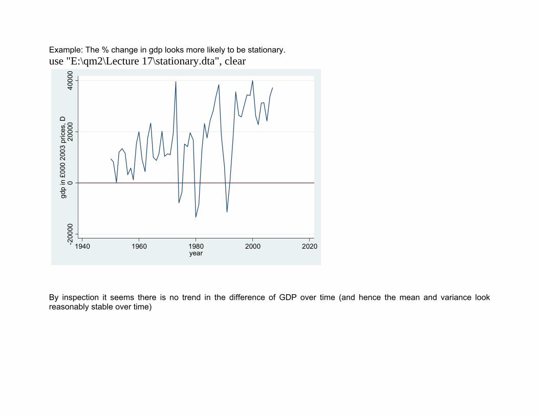
Example: The % change in gdp looks more likely to be stationary. use "E:\qm2\Lecture 17\stationary.dta", clear
-200
000
2000
040
000
gdp
in £
000
2003
pric
es, D
1940 1960 1980 2000 2020year
By inspection it seems there is no trend in the difference of GDP over time (and hence the mean and variance look reasonably stable over time)
Note: Sometimes taking the (natural) log of a series can make the standard deviation of the log of the series constant.
Note: Sometimes taking the (natural) log of a series can make the standard deviation of the log of the series constant. If the series is exponential (as sometimes is GDP) then the log of the series will be linear and the standard deviation of the log across sub-periods will be constant

Note: Sometimes taking the (natural) log of a series can make the standard deviation of the log of the series constant. If the series is exponential (as sometimes is GDP) then the log of the series will be linear and the standard deviation of the log across sub-periods will be constant (if the series changes by the same proportional amount in each period then the log of a series changes by the same amount in each sub-period)
Note: Sometimes taking the (natural) log of a series can make the standard deviation of the log of the series constant. If the series is exponential (as sometimes is GDP) then the log of the series will be linear and the standard deviation of the log across sub-periods will be constant (if the series changes by the same proportional amount in each period then the log of a series changes by the same amount in each sub-period)
In practice not always easy to tell by looking at a series whether it is a random walk (non-stationary) or not. So need to test this formally
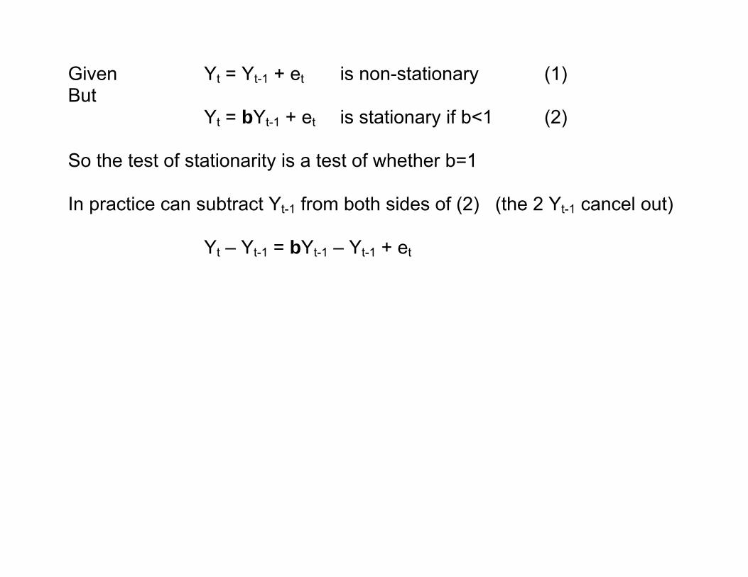
Detection Given Yt = Yt-1 + et is non-stationary (1)
Detection Given Yt = Yt-1 + et is non-stationary (1) But
Yt = bYt-1 + et is stationary if b<1 (2)
(can show the variance of Y is constant for (2) )
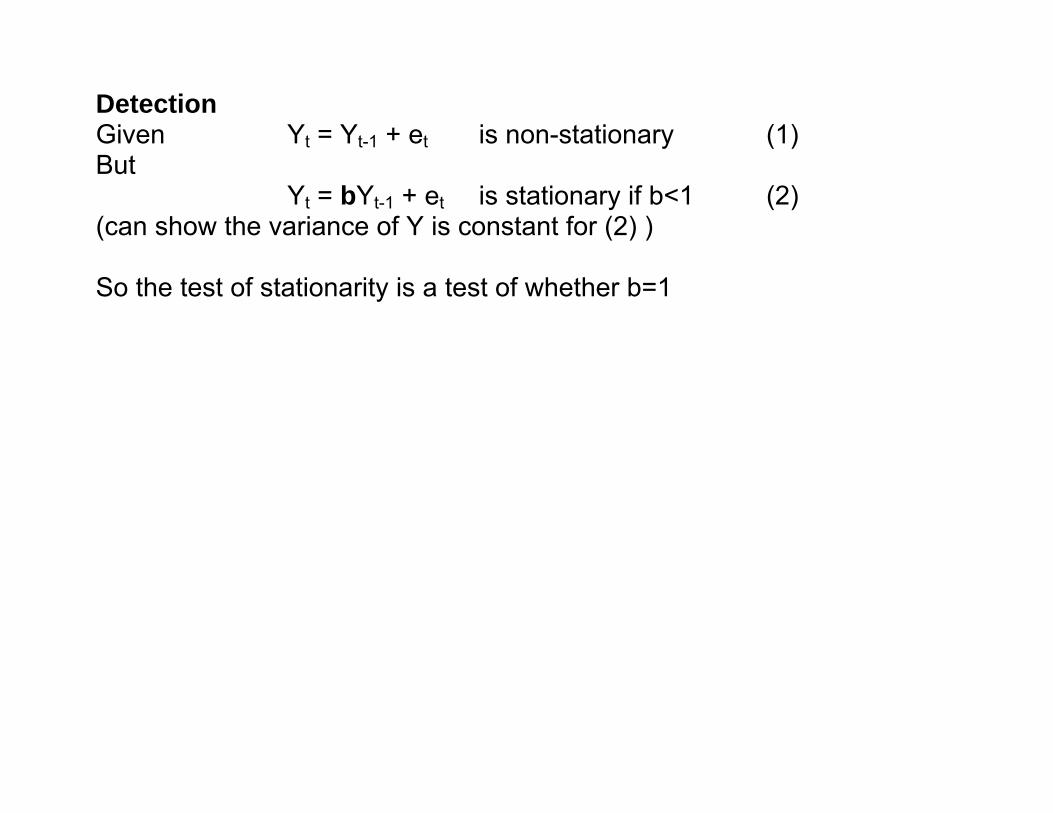
Detection Given Yt = Yt-1 + et is non-stationary (1) But
Yt = bYt-1 + et is stationary if b<1 (2) (can show the variance of Y is constant for (2) ) So the test of stationarity is a test of whether b=1
Detection Given Yt = Yt-1 + et is non-stationary (1) But
Yt = bYt-1 + et is stationary if b<1 (2)
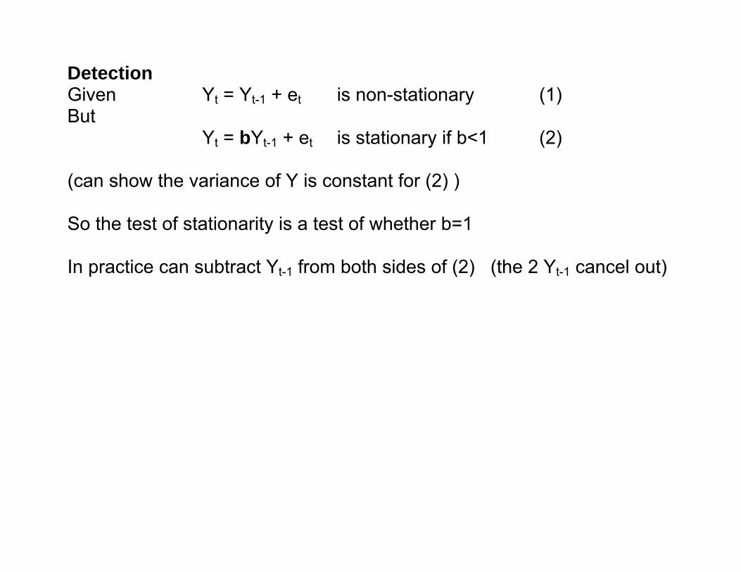
(can show the variance of Y is constant for (2) ) So the test of stationarity is a test of whether b=1 In practice can subtract Yt-1 from both sides of (2) (the 2 Yt-1 cancel out)
Detection Given Yt = Yt-1 + et is non-stationary (1) But
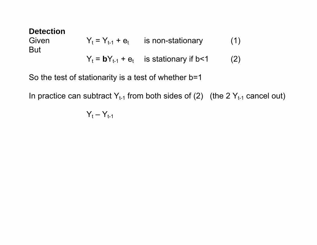
Yt = bYt-1 + et is stationary if b<1 (2)
So the test of stationarity is a test of whether b=1 In practice can subtract Yt-1 from both sides of (2) (the 2 Yt-1 cancel out)
Yt – Yt-1
Given Yt = Yt-1 + et is non-stationary (1) But
Yt = bYt-1 + et is stationary if b<1 (2)
So the test of stationarity is a test of whether b=1 In practice can subtract Yt-1 from both sides of (2) (the 2 Yt-1 cancel out)
Yt – Yt-1 = bYt-1 – Yt-1 + et
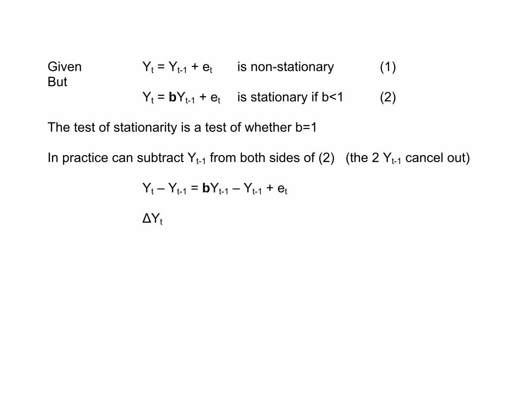
Given Yt = Yt-1 + et is non-stationary (1) But
Yt = bYt-1 + et is stationary if b<1 (2)
The test of stationarity is a test of whether b=1 In practice can subtract Yt-1 from both sides of (2) (the 2 Yt-1 cancel out)
Yt – Yt-1 = bYt-1 – Yt-1 + et
ΔYt
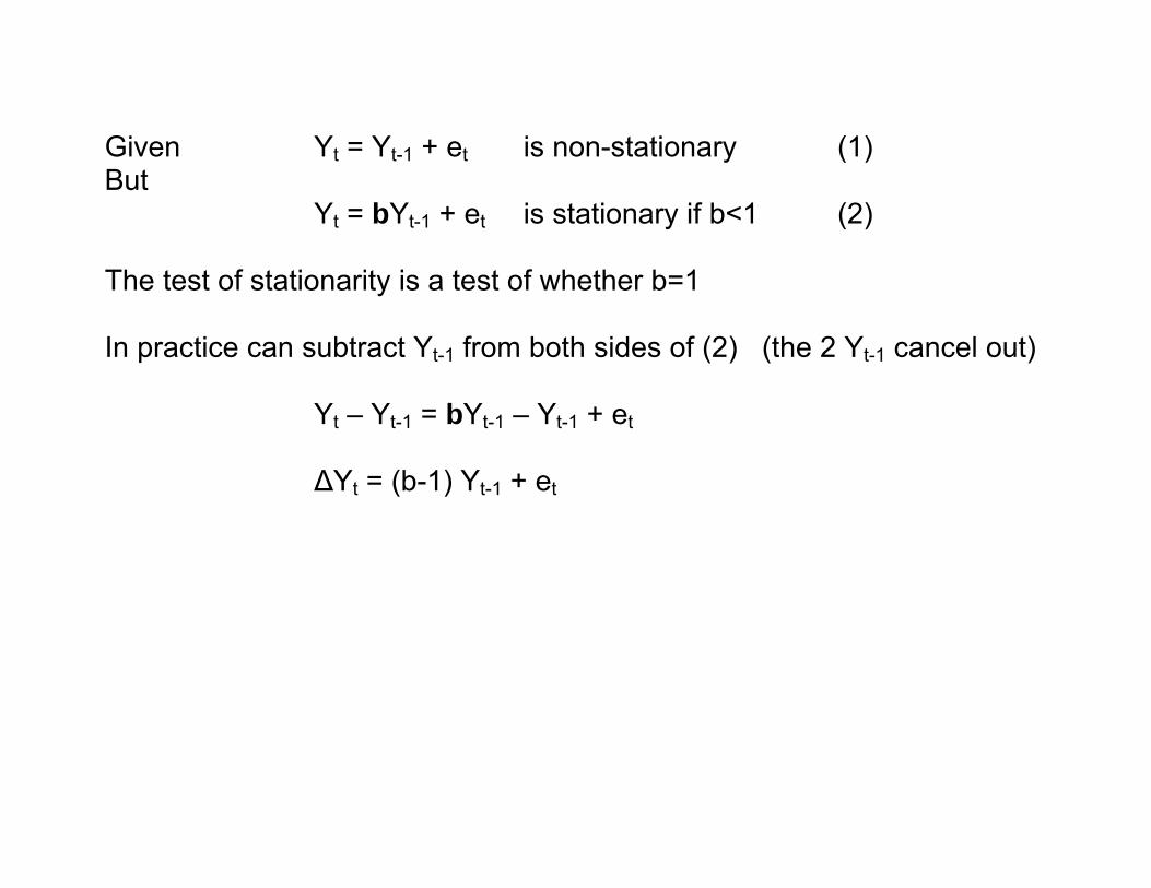
Given Yt = Yt-1 + et is non-stationary (1) But
Yt = bYt-1 + et is stationary if b<1 (2)
The test of stationarity is a test of whether b=1 In practice can subtract Yt-1 from both sides of (2) (the 2 Yt-1 cancel out)
Yt – Yt-1 = bYt-1 – Yt-1 + et
ΔYt = (b-1) Yt-1 + et
Given Yt = Yt-1 + et is non-stationary (1) But
Yt = bYt-1 + et is stationary if b<1 (2)
The test of stationarity is a test of whether b=1 In practice can subtract Yt-1 from both sides of (2) (the 2 Yt-1 cancel out)
Yt – Yt-1 = bYt-1 – Yt-1 + et
ΔYt = (b-1) Yt-1 + et ΔYt = gYt-1 + et (3)
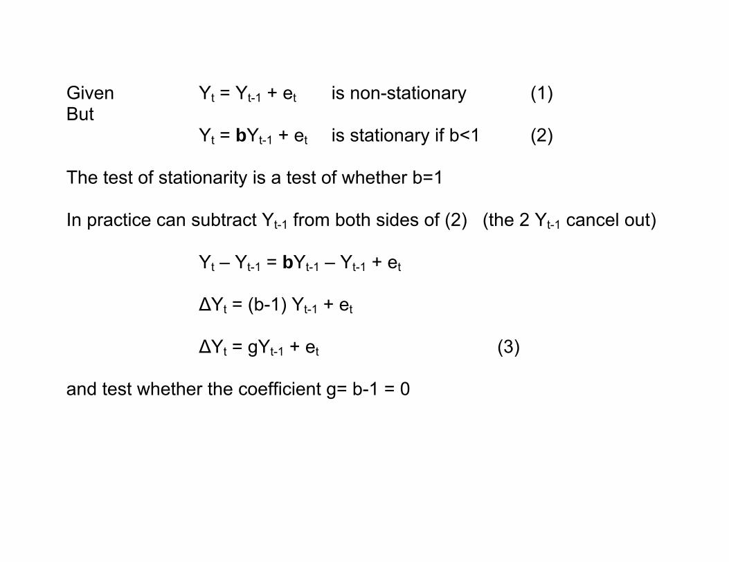
Given Yt = Yt-1 + et is non-stationary (1) But
Yt = bYt-1 + et is stationary if b<1 (2)
The test of stationarity is a test of whether b=1 In practice can subtract Yt-1 from both sides of (2) (the 2 Yt-1 cancel out)
Yt – Yt-1 = bYt-1 – Yt-1 + et
ΔYt = (b-1) Yt-1 + et ΔYt = gYt-1 + et (3)
and test whether the coefficient g= b-1 = 0
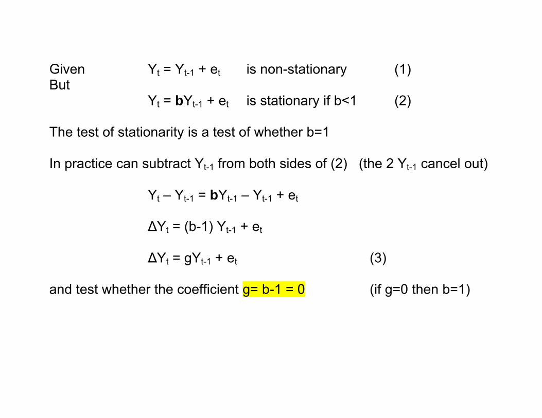
Given Yt = Yt-1 + et is non-stationary (1) But
Yt = bYt-1 + et is stationary if b<1 (2)
The test of stationarity is a test of whether b=1 In practice can subtract Yt-1 from both sides of (2) (the 2 Yt-1 cancel out)
Yt – Yt-1 = bYt-1 – Yt-1 + et
ΔYt = (b-1) Yt-1 + et ΔYt = gYt-1 + et (3)
and test whether the coefficient g= b-1 = 0 (if g=0 then b=1)
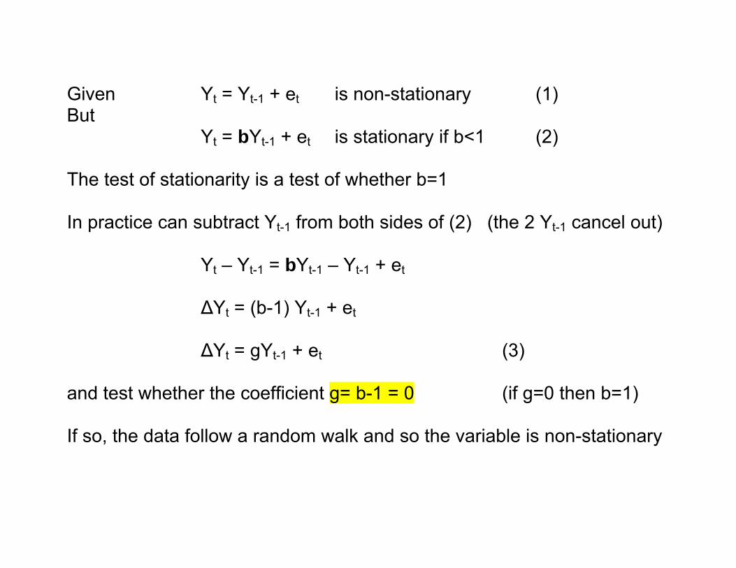
Given Yt = Yt-1 + et is non-stationary (1) But
Yt = bYt-1 + et is stationary if b<1 (2)
The test of stationarity is a test of whether b=1 In practice can subtract Yt-1 from both sides of (2) (the 2 Yt-1 cancel out)
Yt – Yt-1 = bYt-1 – Yt-1 + et
ΔYt = (b-1) Yt-1 + et ΔYt = gYt-1 + et (3)
and test whether the coefficient g= b-1 = 0 (if g=0 then b=1) If so, the data follow a random walk and so the variable is non-stationary
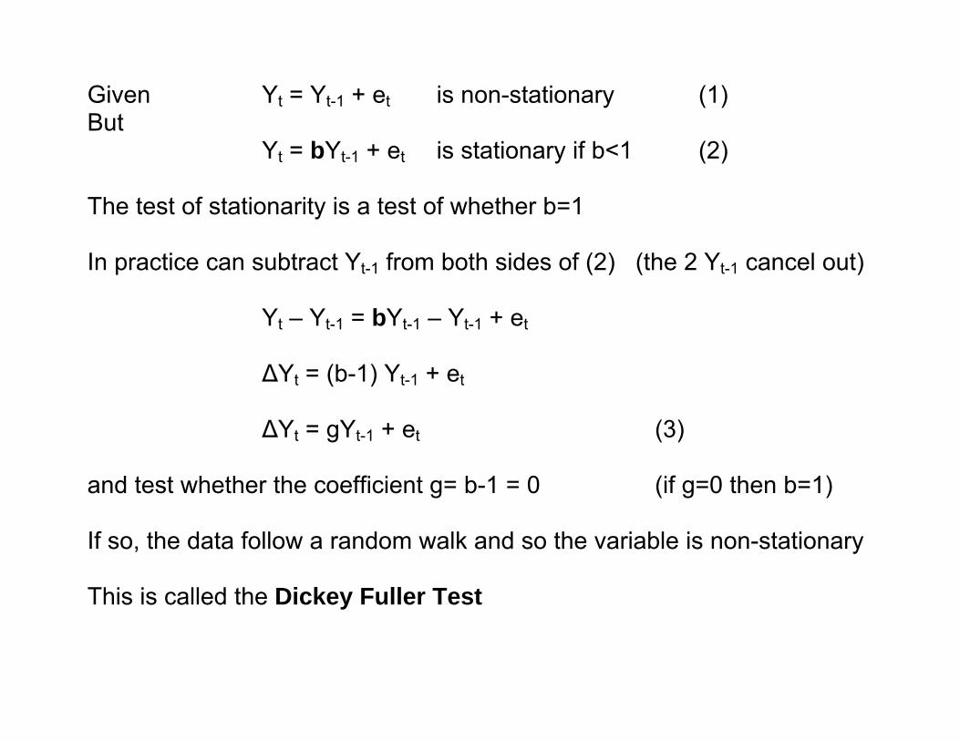
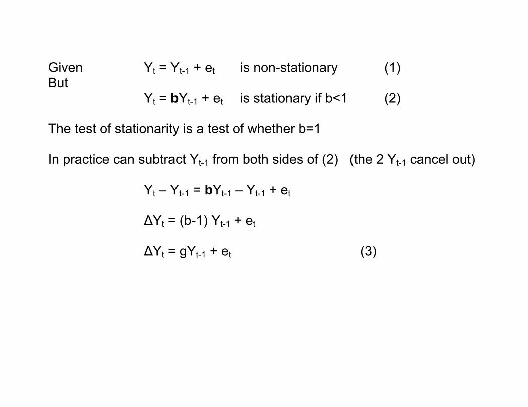
Given Yt = Yt-1 + et is non-stationary (1) But
Yt = bYt-1 + et is stationary if b<1 (2)
The test of stationarity is a test of whether b=1 In practice can subtract Yt-1 from both sides of (2) (the 2 Yt-1 cancel out)
Yt – Yt-1 = bYt-1 – Yt-1 + et
ΔYt = (b-1) Yt-1 + et ΔYt = gYt-1 + et (3)
and test whether the coefficient g= b-1 = 0 (if g=0 then b=1) If so, the data follow a random walk and so the variable is non-stationary This is called the Dickey Fuller Test
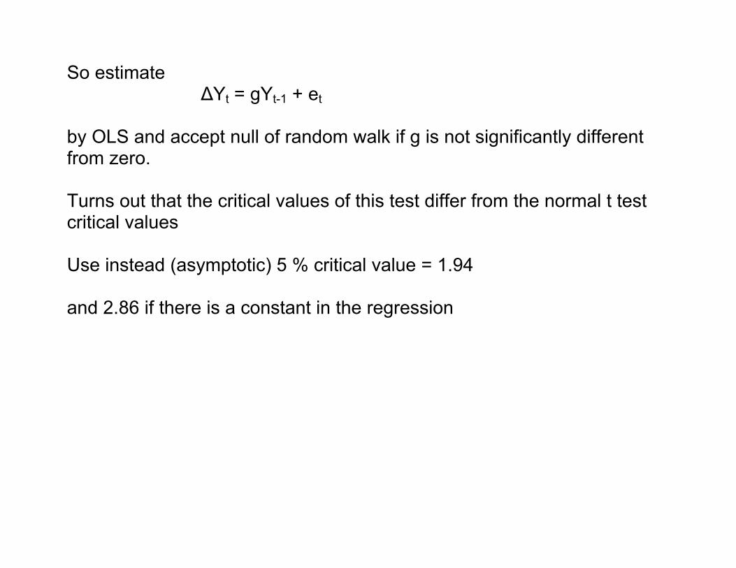
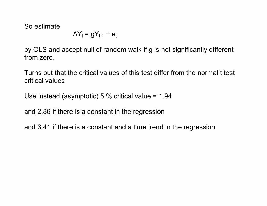
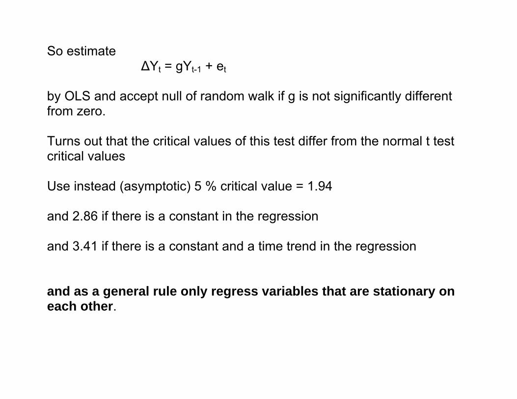
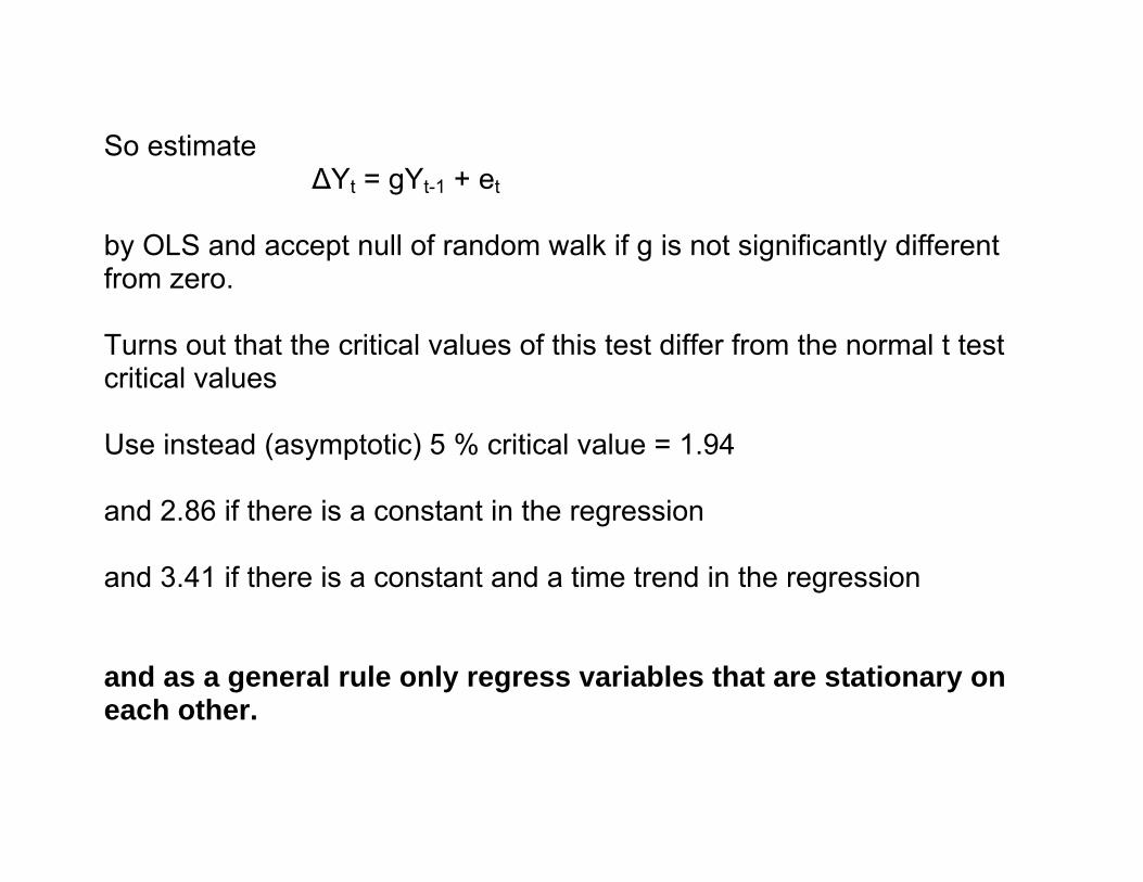
So estimate ΔYt = gYt-1 + et
by OLS and accept null of random walk if g is not significantly different from zero.
So estimate ΔYt = gYt-1 + et
by OLS and accept null of random walk if g is not significantly different from zero. Turns out that the critical values of this test differ from the normal t test critical values
So estimate ΔYt = gYt-1 + et
by OLS and accept null of random walk if g is not significantly different from zero. Turns out that the critical values of this test differ from the normal t test critical values Use instead (asymptotic) 5 % critical value = 1.94 and 2.86 if there is a constant in the regression
So estimate ΔYt = gYt-1 + et
by OLS and accept null of random walk if g is not significantly different from zero. Turns out that the critical values of this test differ from the normal t test critical values Use instead (asymptotic) 5 % critical value = 1.94 and 2.86 if there is a constant in the regression and 3.41 if there is a constant and a time trend in the regression
So estimate ΔYt = gYt-1 + et
by OLS and accept null of random walk if g is not significantly different from zero. Turns out that the critical values of this test differ from the normal t test critical values Use instead (asymptotic) 5 % critical value = 1.94 and 2.86 if there is a constant in the regression and 3.41 if there is a constant and a time trend in the regression and as a general rule only regress variables that are stationary on each other.
So estimate
ΔYt = gYt-1 + et by OLS and accept null of random walk if g is not significantly different from zero. Turns out that the critical values of this test differ from the normal t test critical values Use instead (asymptotic) 5 % critical value = 1.94 and 2.86 if there is a constant in the regression and 3.41 if there is a constant and a time trend in the regression and as a general rule only regress variables that are stationary on each other.
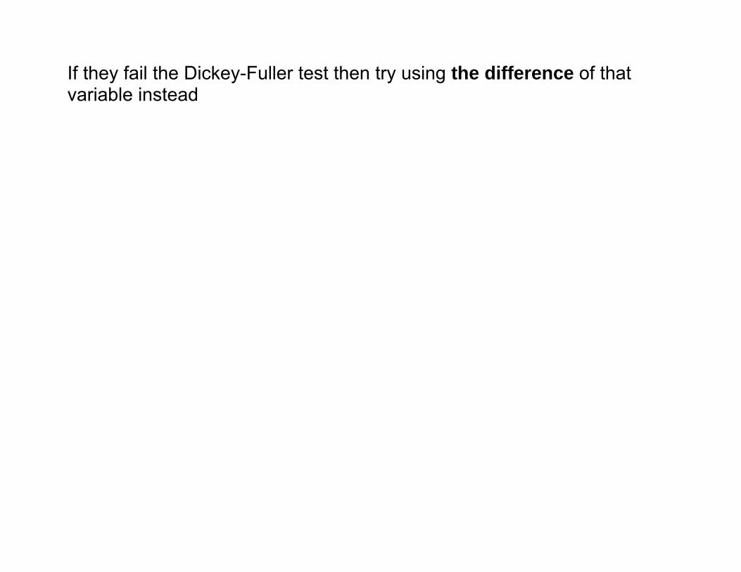
If they fail the Dickey-Fuller test then try using the difference of that variable instead
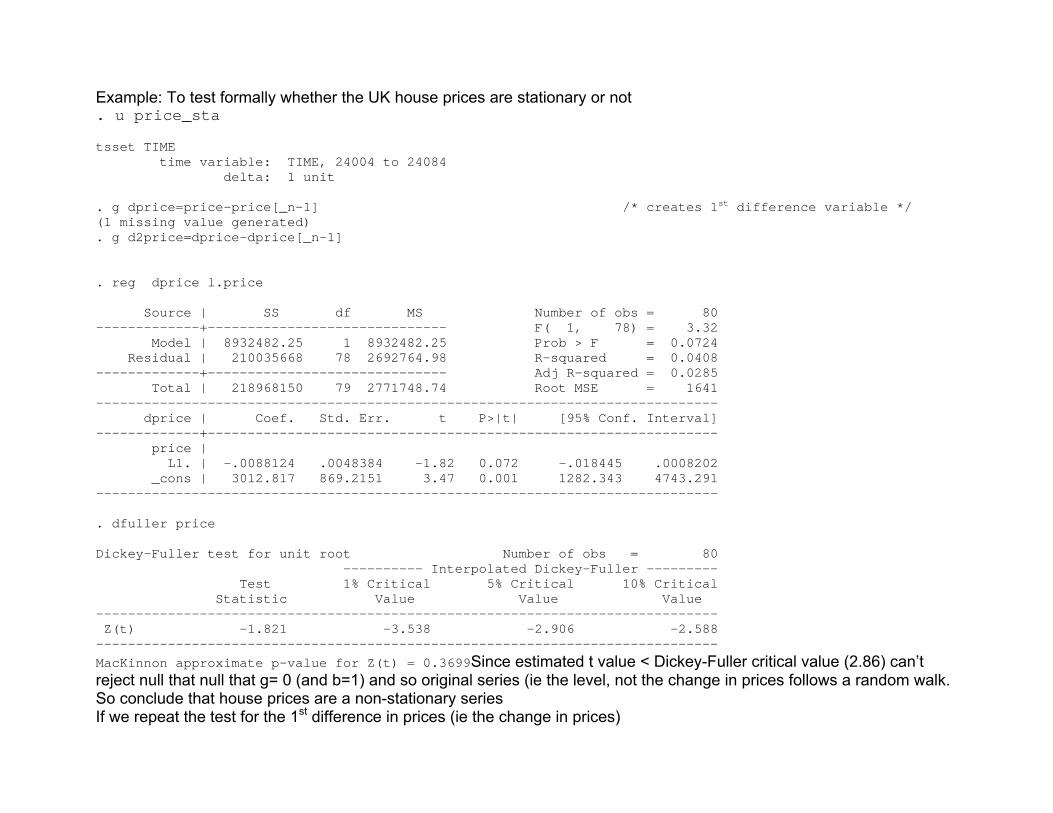
Example: To test formally whether the UK house prices are stationary or not . u price_sta tsset TIME time variable: TIME, 24004 to 24084 delta: 1 unit . g dprice=price-price[_n-1] /* creates 1st difference variable */ (1 missing value generated) . g d2price=dprice-dprice[_n-1] . reg dprice l.price Source | SS df MS Number of obs = 80 -------------+------------------------------ F( 1, 78) = 3.32 Model | 8932482.25 1 8932482.25 Prob > F = 0.0724 Residual | 210035668 78 2692764.98 R-squared = 0.0408 -------------+------------------------------ Adj R-squared = 0.0285 Total | 218968150 79 2771748.74 Root MSE = 1641 ------------------------------------------------------------------------------ dprice | Coef. Std. Err. t P>|t| [95% Conf. Interval] -------------+---------------------------------------------------------------- price | L1. | -.0088124 .0048384 -1.82 0.072 -.018445 .0008202 _cons | 3012.817 869.2151 3.47 0.001 1282.343 4743.291 ------------------------------------------------------------------------------ . dfuller price Dickey-Fuller test for unit root Number of obs = 80 ---------- Interpolated Dickey-Fuller --------- Test 1% Critical 5% Critical 10% Critical Statistic Value Value Value ------------------------------------------------------------------------------ Z(t) -1.821 -3.538 -2.906 -2.588 ------------------------------------------------------------------------------ MacKinnon approximate p-value for Z(t) = 0.3699Since estimated t value < Dickey-Fuller critical value (2.86) can’t reject null that null that g= 0 (and b=1) and so original series (ie the level, not the change in prices follows a random walk. So conclude that house prices are a non-stationary series If we repeat the test for the 1st difference in prices (ie the change in prices)
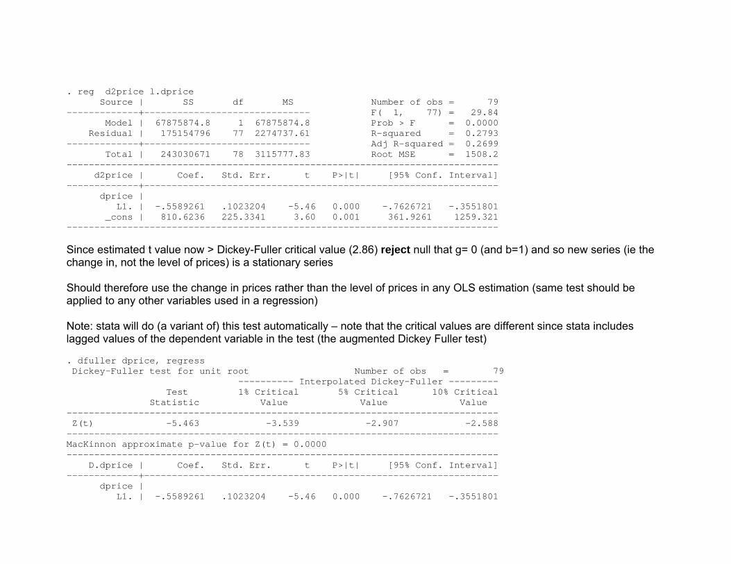
. reg d2price l.dprice Source | SS df MS Number of obs = 79 -------------+------------------------------ F( 1, 77) = 29.84 Model | 67875874.8 1 67875874.8 Prob > F = 0.0000 Residual | 175154796 77 2274737.61 R-squared = 0.2793 -------------+------------------------------ Adj R-squared = 0.2699 Total | 243030671 78 3115777.83 Root MSE = 1508.2 ------------------------------------------------------------------------------ d2price | Coef. Std. Err. t P>|t| [95% Conf. Interval] -------------+---------------------------------------------------------------- dprice | L1. | -.5589261 .1023204 -5.46 0.000 -.7626721 -.3551801 _cons | 810.6236 225.3341 3.60 0.001 361.9261 1259.321 ------------------------------------------------------------------------------ Since estimated t value now > Dickey-Fuller critical value (2.86) reject null that g= 0 (and b=1) and so new series (ie the change in, not the level of prices) is a stationary series Should therefore use the change in prices rather than the level of prices in any OLS estimation (same test should be applied to any other variables used in a regression) Note: stata will do (a variant of) this test automatically – note that the critical values are different since stata includes lagged values of the dependent variable in the test (the augmented Dickey Fuller test) . dfuller dprice, regress Dickey-Fuller test for unit root Number of obs = 79 ---------- Interpolated Dickey-Fuller --------- Test 1% Critical 5% Critical 10% Critical Statistic Value Value Value ------------------------------------------------------------------------------ Z(t) -5.463 -3.539 -2.907 -2.588 ------------------------------------------------------------------------------ MacKinnon approximate p-value for Z(t) = 0.0000 ------------------------------------------------------------------------------ D.dprice | Coef. Std. Err. t P>|t| [95% Conf. Interval] -------------+---------------------------------------------------------------- dprice | L1. | -.5589261 .1023204 -5.46 0.000 -.7626721 -.3551801
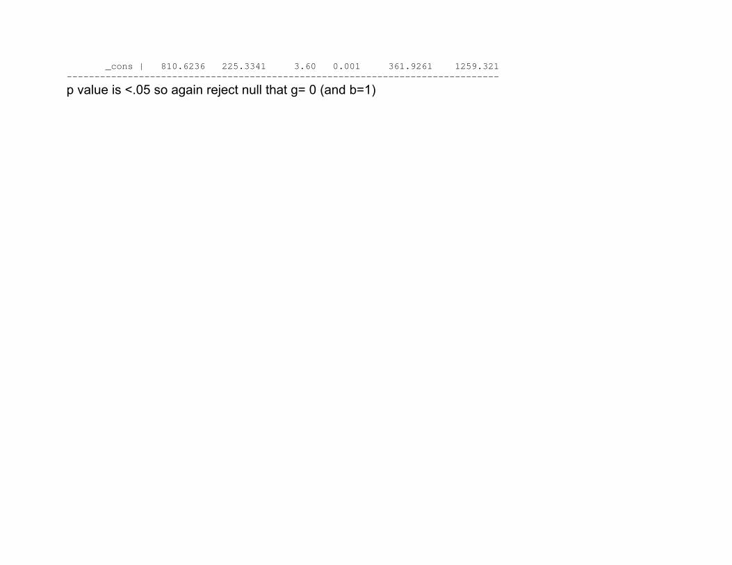
_cons | 810.6236 225.3341 3.60 0.001 361.9261 1259.321 ------------------------------------------------------------------------------
p value is <.05 so again reject null that g= 0 (and b=1)
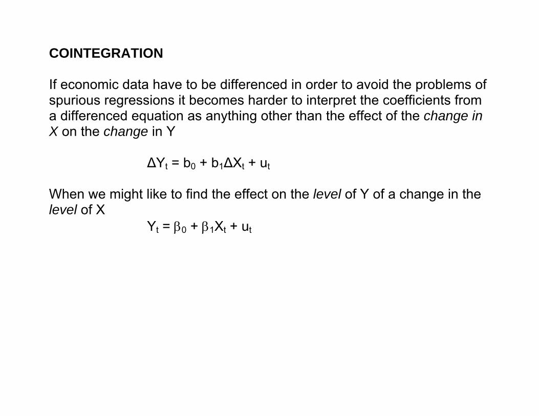
COINTEGRATION If economic data have to be differenced in order to avoid the problems of spurious regressions it becomes harder to interpret the coefficients from a differenced equation as anything other than the effect of the change in X on the change in Y ΔYt = b0 + b1ΔXt + ut When we might like to find the effect on the level of Y of a change in the level of X Yt = β0 + β1Xt + ut
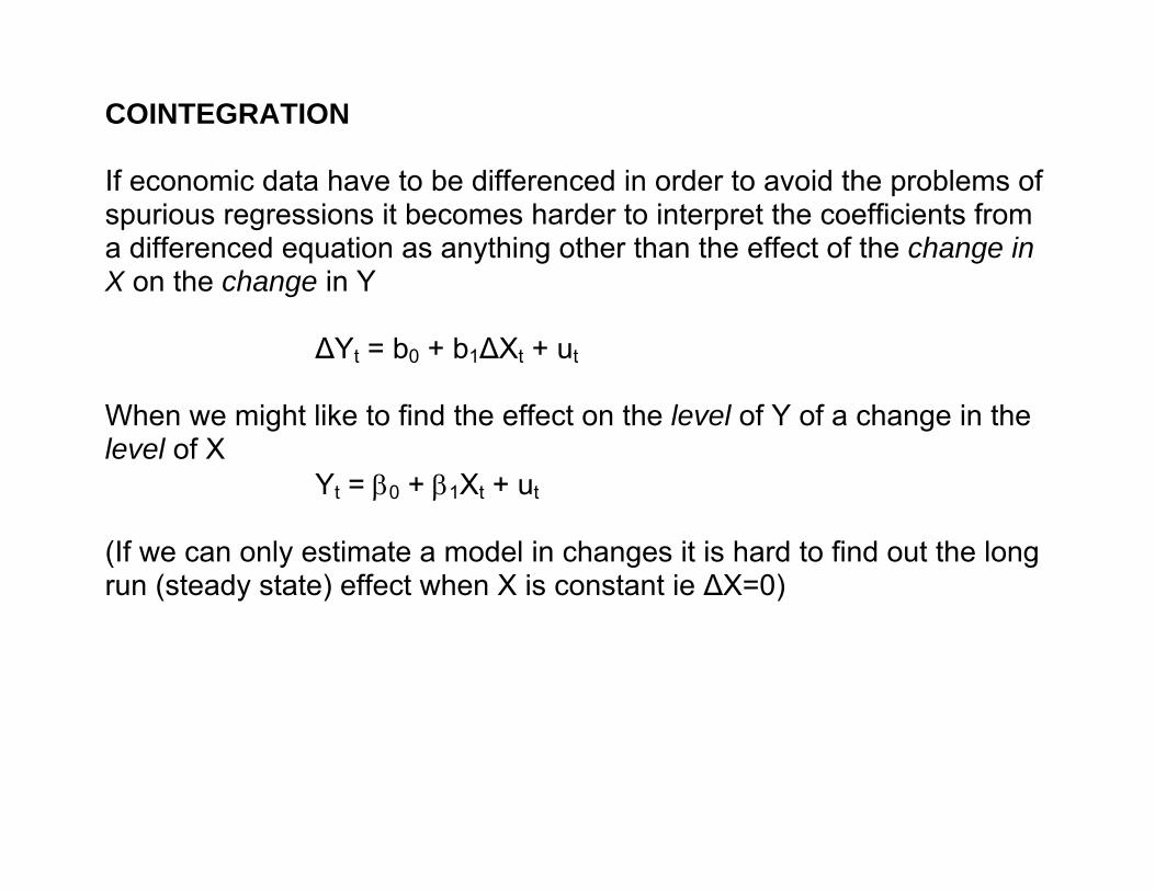
COINTEGRATION If economic data have to be differenced in order to avoid the problems of spurious regressions it becomes harder to interpret the coefficients from a differenced equation as anything other than the effect of the change in X on the change in Y ΔYt = b0 + b1ΔXt + ut When we might like to find the effect on the level of Y of a change in the level of X Yt = β0 + β1Xt + ut (If we can only estimate a model in changes it is hard to find out the long run (steady state) effect when X is constant ie ΔX=0)
COINTEGRATION If economic data have to be differenced in order to avoid the problems of spurious regressions it becomes harder to interpret the coefficients from a differenced equation as anything other than the effect of the change in X on the change in Y ΔYt = b0 + b1ΔXt + ut When we might like to find the effect on the level of Y of a change in the level of X Yt = β0 + β1Xt + ut (If we can only estimate a model in changes it is hard to find out the long run (steady state) effect when X is constant ie ΔX=0) However if a long-run relationship exists, the 2 variables are said to be cointegrated. The trick is to try and tease out the long-run relationship. variables with a common trend are also said to be cointegrated
If 2 non-stationary variables have a common trend then we can net it out (like in the Dickey-Fuller test) by using some function of the difference in the 2 series Yt - δXt where δ is some constant This difference term will, in general, be stationary and so can be added to a model ΔYt = b0 + b1ΔXt + b2(Yt - δXt) ut The usefulness of this procedure lies in the fact that the coefficient b2 is called the error correction effect and it can be used to assess the extent of movement of y to its long run equilibrium value following a change in X
day
onemonth oneyear
1 25 50 75 100
4
4.2
4.4
4.6
4.8
5
5.2
5.4
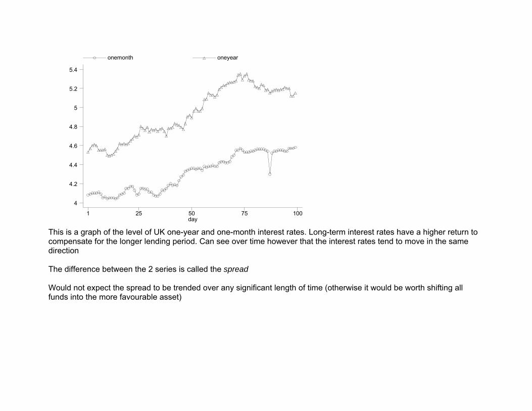
This is a graph of the level of UK one-year and one-month interest rates. Long-term interest rates have a higher return to compensate for the longer lending period. Can see over time however that the interest rates tend to move in the same direction The difference between the 2 series is called the spread Would not expect the spread to be trended over any significant length of time (otherwise it would be worth shifting all funds into the more favourable asset)
spre
ad
day1 25 50 75 100
.4
.5
.6
.7
.8
.9
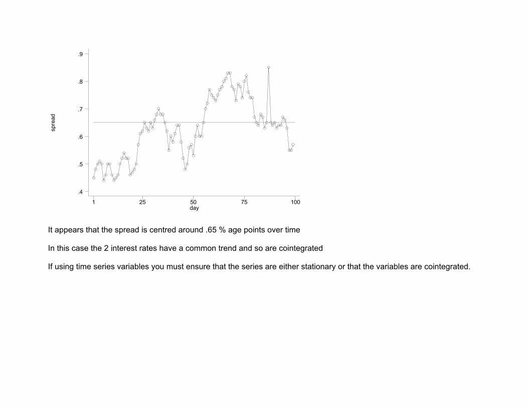
It appears that the spread is centred around .65 % age points over time In this case the 2 interest rates have a common trend and so are cointegrated If using time series variables you must ensure that the series are either stationary or that the variables are cointegrated.
Another way to do this is to look at the behaviour of the residual from the model Yt = b0 + b1Xt +ut Suppose Y band X are non-stationary, but related. If so then any residual should be not be systematic (ie random)
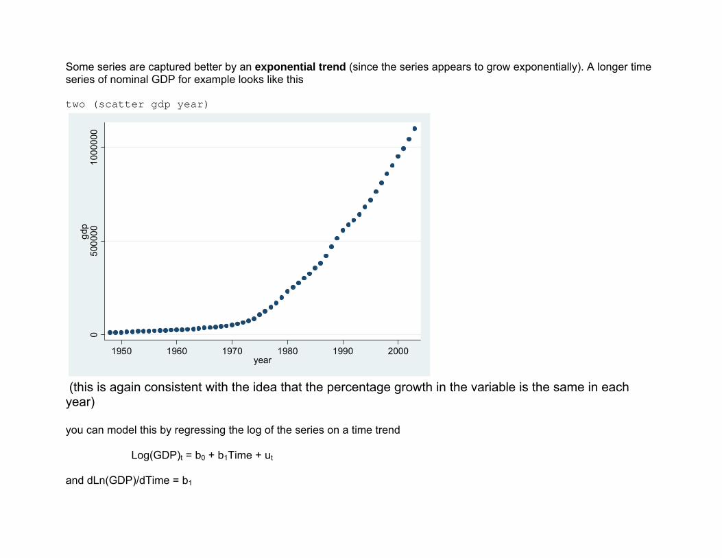
Some series are captured better by an exponential trend (since the series appears to grow exponentially). A longer time series of nominal GDP for example looks like this two (scatter gdp year)
050
0000
1000
000
gdp
1950 1960 1970 1980 1990 2000year
(this is again consistent with the idea that the percentage growth in the variable is the same in each year) you can model this by regressing the log of the series on a time trend Log(GDP)t = b0 + b1Time + ut
and dLn(GDP)/dTime = b1
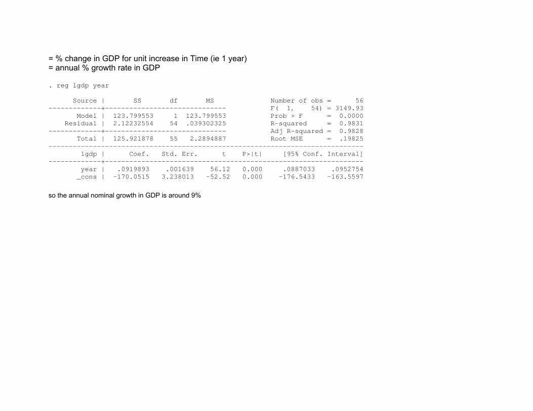
= % change in GDP for unit increase in Time (ie 1 year) = annual % growth rate in GDP . reg lgdp year Source | SS df MS Number of obs = 56 -------------+------------------------------ F( 1, 54) = 3149.93 Model | 123.799553 1 123.799553 Prob > F = 0.0000 Residual | 2.12232554 54 .039302325 R-squared = 0.9831 -------------+------------------------------ Adj R-squared = 0.9828 Total | 125.921878 55 2.2894887 Root MSE = .19825 ------------------------------------------------------------------------------ lgdp | Coef. Std. Err. t P>|t| [95% Conf. Interval] -------------+---------------------------------------------------------------- year | .0919893 .001639 56.12 0.000 .0887033 .0952754 _cons | -170.0515 3.238013 -52.52 0.000 -176.5433 -163.5597
so the annual nominal growth in GDP is around 9%