Lecture 17 Instructor : Mert Pilanci
67
EE269 Signal Processing for Machine Learning Lecture 17 Instructor : Mert Pilanci Stanford University November 18, 2020
Transcript of Lecture 17 Instructor : Mert Pilanci
EE269Signal Processing for Machine Learning
Lecture 17
Instructor : Mert Pilanci
Stanford University
November 18, 2020
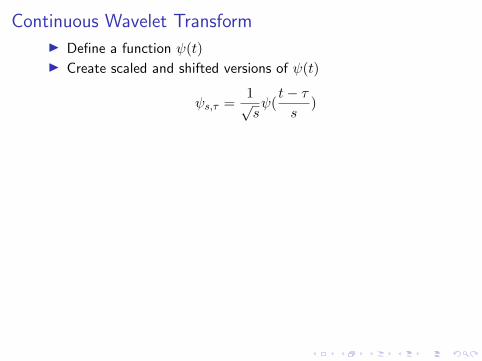
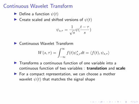
Continuous Wavelet Transform
I Define a function ψ(t)I Create scaled and shifted versions of ψ(t)
ψs,τ =1√sψ(t− τs
)
I Continuous Wavelet Transform
W (s, τ) =
∫ ∞−∞
f(t)ψ∗s,τdt = 〈f(t), ψs,τ 〉
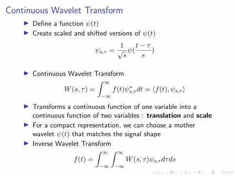
I Transforms a continuous function of one variable into acontinuous function of two variables : translation and scale
I For a compact representation, we can choose a motherwavelet ψ(t) that matches the signal shape
I Inverse Wavelet Transform
f(t) =
∫ ∞−∞
∫ ∞−∞
W (s, τ)ψs,τdτds
Continuous Wavelet Transform
I Define a function ψ(t)I Create scaled and shifted versions of ψ(t)
ψs,τ =1√sψ(t− τs
)
I Continuous Wavelet Transform
W (s, τ) =
∫ ∞−∞
f(t)ψ∗s,τdt = 〈f(t), ψs,τ 〉
I Transforms a continuous function of one variable into acontinuous function of two variables : translation and scale
I For a compact representation, we can choose a motherwavelet ψ(t) that matches the signal shape
I Inverse Wavelet Transform
f(t) =
∫ ∞−∞
∫ ∞−∞
W (s, τ)ψs,τdτds
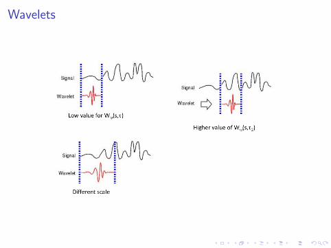
Wavelets
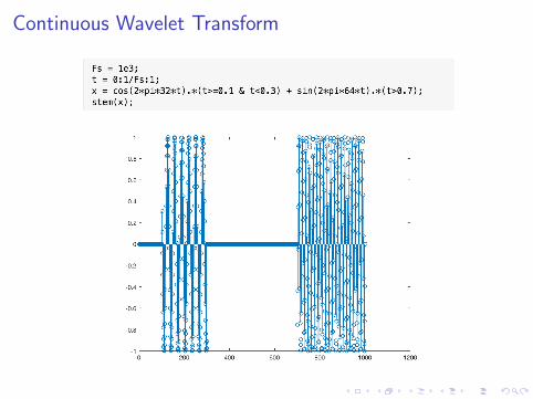
Continuous Wavelet Transform
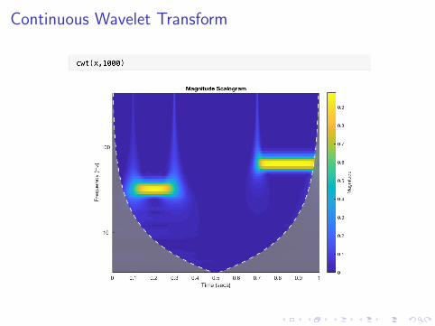
Continuous Wavelet Transform
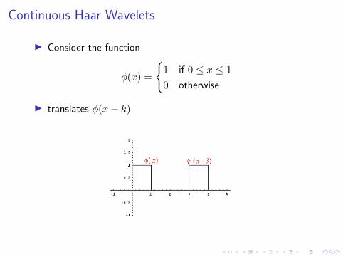
Continuous Haar Wavelets
I Consider the function
φ(x) =
{1 if 0 ≤ x ≤ 1
0 otherwise
I translates φ(x− k)
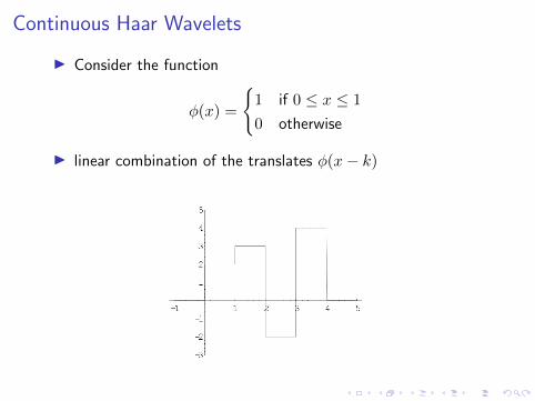
Continuous Haar Wavelets
I Consider the function
φ(x) =
{1 if 0 ≤ x ≤ 1
0 otherwise
I linear combination of the translates φ(x− k)
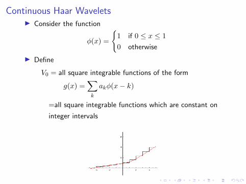
Continuous Haar WaveletsI Consider the function
φ(x) =
{1 if 0 ≤ x ≤ 1
0 otherwise
I Define
V0 = all square integrable functions of the form
g(x) =∑k
akφ(x− k)
=all square integrable functions which are constant on
integer intervals
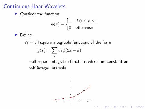
Continuous Haar WaveletsI Consider the function
φ(x) =
{1 if 0 ≤ x ≤ 1
0 otherwise
I Define
V1 = all square integrable functions of the form
g(x) =∑k
akφ(2x− k)
=all square integrable functions which are constant on
half integer intervals
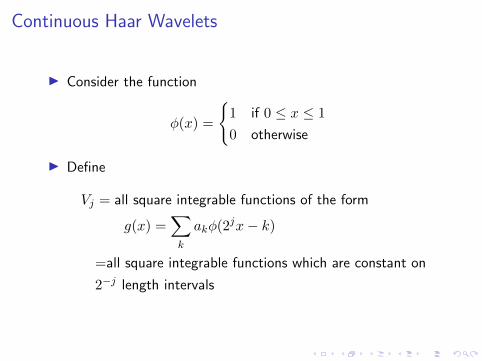
Continuous Haar Wavelets
I Consider the function
φ(x) =
{1 if 0 ≤ x ≤ 1
0 otherwise
I Define
Vj = all square integrable functions of the form
g(x) =∑k
akφ(2jx− k)
=all square integrable functions which are constant on
2−j length intervals
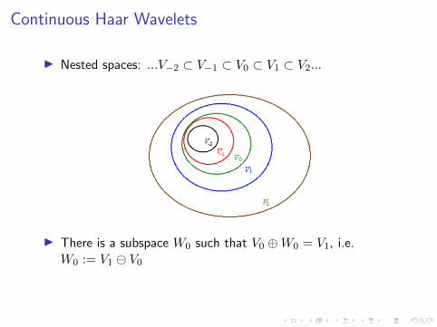
Continuous Haar Wavelets
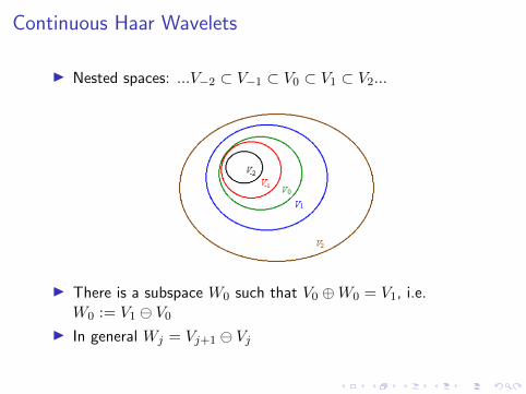
I Nested spaces: ...V−2 ⊂ V−1 ⊂ V0 ⊂ V1 ⊂ V2...
I There is a subspace W0 such that V0 ⊕W0 = V1, i.e.W0 := V1 V0
I In general Wj = Vj+1 Vj
Continuous Haar Wavelets
I Nested spaces: ...V−2 ⊂ V−1 ⊂ V0 ⊂ V1 ⊂ V2...
I There is a subspace W0 such that V0 ⊕W0 = V1, i.e.W0 := V1 V0
I In general Wj = Vj+1 Vj

Continuous Haar Wavelets
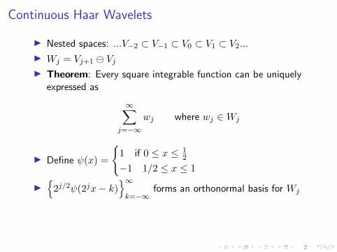
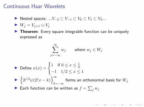
I Nested spaces: ...V−2 ⊂ V−1 ⊂ V0 ⊂ V1 ⊂ V2...
I Wj = Vj+1 VjI Theorem: Every square integrable function can be uniquely
expressed as
∞∑j=−∞
wj where wj ∈Wj
Continuous Haar Wavelets
I Nested spaces: ...V−2 ⊂ V−1 ⊂ V0 ⊂ V1 ⊂ V2...I Wj = Vj+1 VjI Theorem: Every square integrable function can be uniquely
expressed as
∞∑j=−∞
wj where wj ∈Wj
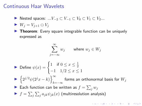
I Define ψ(x) =
{1 if 0 ≤ x ≤ 1
2
−1 1/2 ≤ x ≤ 1
I{2j/2ψ(2jx− k)
}∞k=−∞
forms an orthonormal basis for Wj
I Each function can be written as f =∑
j wj
I f =∑
j
∑j ajkψjk(x) (multiresolution analysis)
Continuous Haar Wavelets
I Nested spaces: ...V−2 ⊂ V−1 ⊂ V0 ⊂ V1 ⊂ V2...I Wj = Vj+1 VjI Theorem: Every square integrable function can be uniquely
expressed as
∞∑j=−∞
wj where wj ∈Wj
I Define ψ(x) =
{1 if 0 ≤ x ≤ 1
2
−1 1/2 ≤ x ≤ 1
I{2j/2ψ(2jx− k)
}∞k=−∞
forms an orthonormal basis for Wj
I Each function can be written as f =∑
j wj
I f =∑
j
∑j ajkψjk(x) (multiresolution analysis)
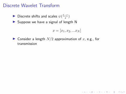
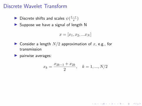
Discrete Wavelet Transform
I Discrete shifts and scales ψ( t−τs )
I Suppose we have a signal of length N
x = [x1, x2, ...xN ]
I Consider a length N/2 approximation of x, e.g., fortransmission
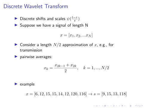
I pairwise averages:
xk =x2k−1 + x2k
2, k = 1, ..., N/2
I example
x = [6, 12, 15, 15, 14, 12, 120, 116]→ s = [9, 15, 13, 118]
Discrete Wavelet Transform
I Discrete shifts and scales ψ( t−τs )
I Suppose we have a signal of length N
x = [x1, x2, ...xN ]
I Consider a length N/2 approximation of x, e.g., fortransmission
I pairwise averages:
xk =x2k−1 + x2k
2, k = 1, ..., N/2
I example
x = [6, 12, 15, 15, 14, 12, 120, 116]→ s = [9, 15, 13, 118]
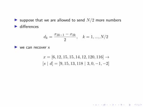
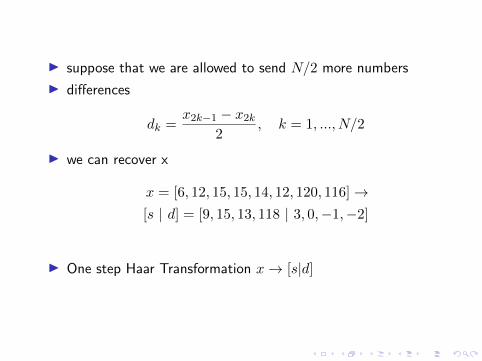
I suppose that we are allowed to send N/2 more numbers
I differences
dk =x2k−1 − x2k
2, k = 1, ..., N/2
I we can recover x
x = [6, 12, 15, 15, 14, 12, 120, 116]→[s | d] = [9, 15, 13, 118 | 3, 0,−1,−2]
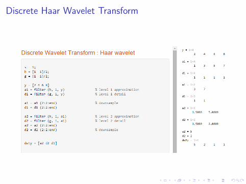
I One step Haar Transformation x→ [s|d]
I suppose that we are allowed to send N/2 more numbers
I differences
dk =x2k−1 − x2k
2, k = 1, ..., N/2
I we can recover x
x = [6, 12, 15, 15, 14, 12, 120, 116]→[s | d] = [9, 15, 13, 118 | 3, 0,−1,−2]
I One step Haar Transformation x→ [s|d]
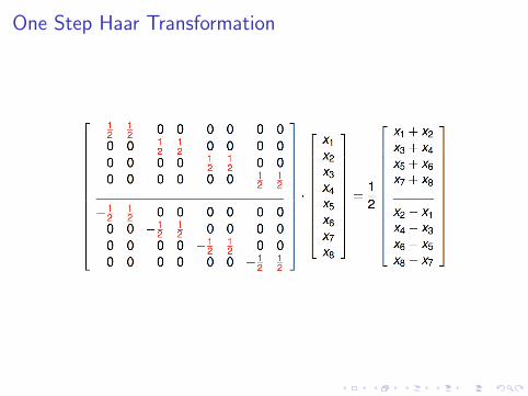
One Step Haar Transformation
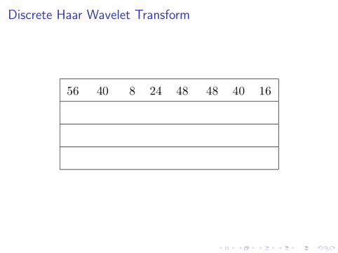
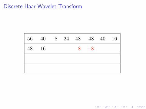
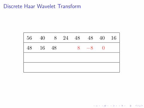
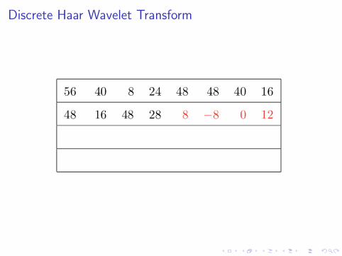
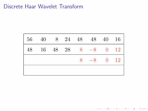
Discrete Haar Wavelet Transform
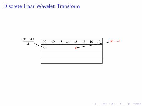
Discrete Haar Wavelet Transform
Discrete Haar Wavelet Transform
Discrete Haar Wavelet Transform
Discrete Haar Wavelet Transform
Discrete Haar Wavelet Transform
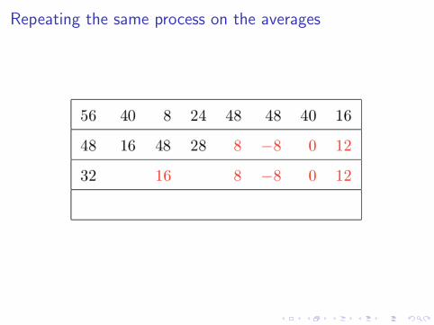
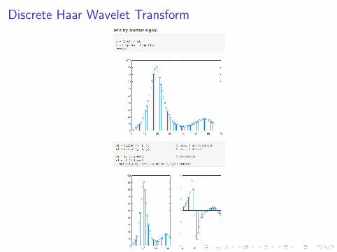
Repeating the same process on the averages
Discrete Haar Wavelet Transform
Discrete Haar Wavelet Transform
Discrete Haar Wavelet Transform
Discrete Haar Wavelet Transform
Discrete Haar Wavelet Transform

Discrete Haar Wavelet Transform
Discrete Haar Wavelet Transform
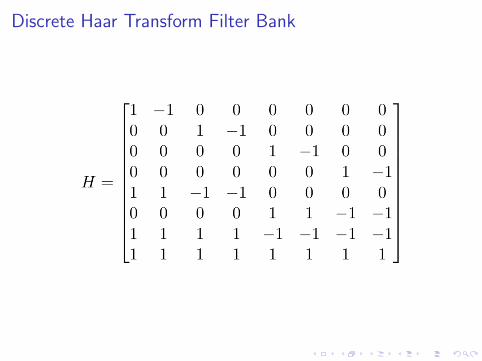
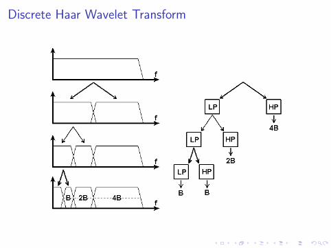
Discrete Haar Transform Filter Bank
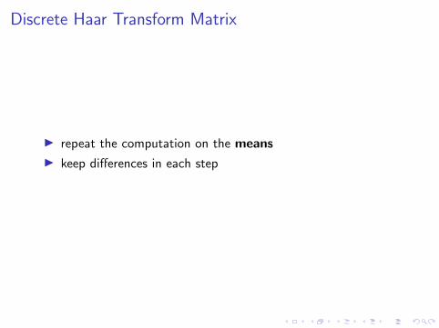
Discrete Haar Transform Matrix
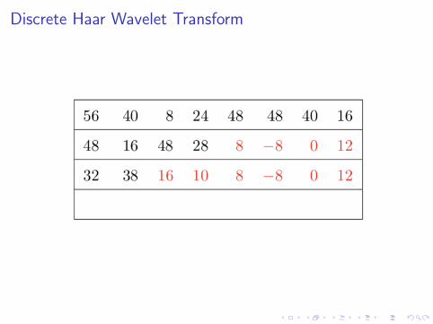
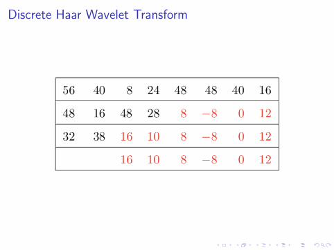
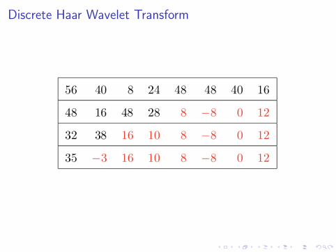
I repeat the computation on the means
I keep differences in each step
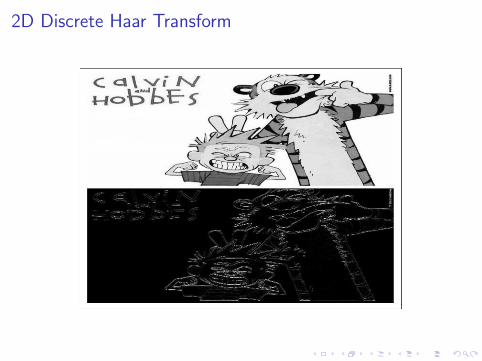
2D Discrete Haar Transform
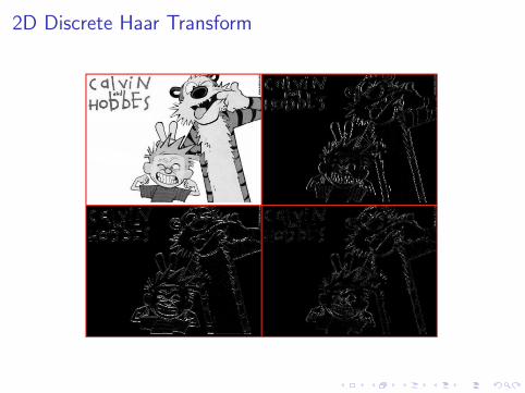
2D Discrete Haar Transform
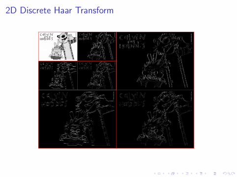
2D Discrete Haar Transform
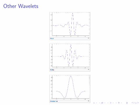
Other Wavelets
Other Wavelets
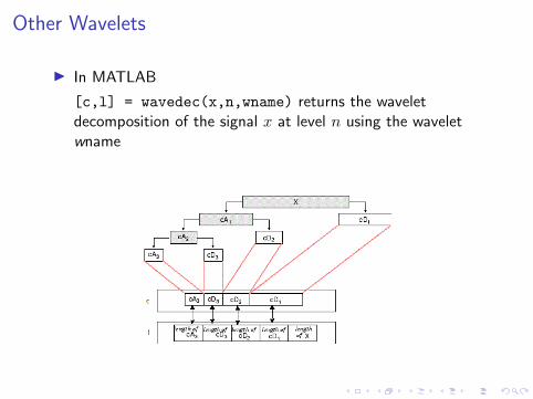
I In MATLAB
[c,l] = wavedec(x,n,wname) returns the waveletdecomposition of the signal x at level n using the waveletwname
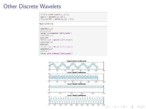
Other Discrete Wavelets
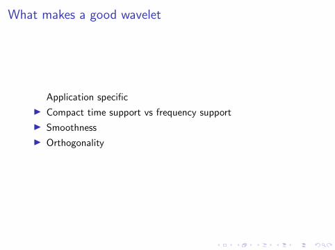
What makes a good wavelet
Application specific
I Compact time support vs frequency support
I Smoothness
I Orthogonality
Fourier vs Wavelet Transforms
I Fourier Transform has convolution theorem and mathematicalrelationships
I No closed form relations exist for wavelet transforms
I Fourier transform has uniform spectral resolution
I Wavelet transform has adaptive resolution
I 100 Hz resolution at 400 Hz and at 4000 Hz are not the same
Short-time Fourier Transform
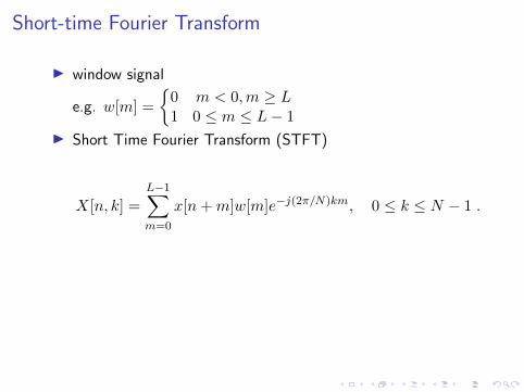
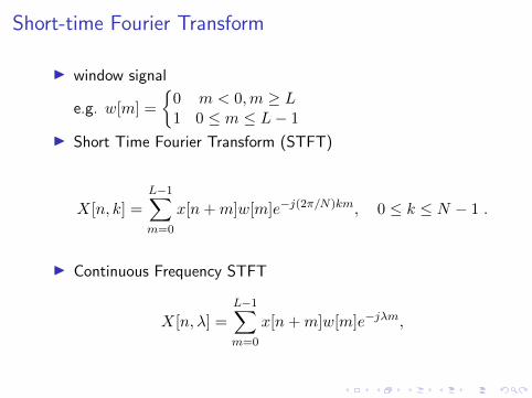
I window signal
e.g. w[m] =
{0 m < 0,m ≥ L1 0 ≤ m ≤ L− 1
I Short Time Fourier Transform (STFT)
X[n, k] =
L−1∑m=0
x[n+m]w[m]e−j(2π/N)km, 0 ≤ k ≤ N − 1 .
I Continuous Frequency STFT
X[n, λ] =L−1∑m=0
x[n+m]w[m]e−jλm,
Short-time Fourier Transform
I window signal
e.g. w[m] =
{0 m < 0,m ≥ L1 0 ≤ m ≤ L− 1
I Short Time Fourier Transform (STFT)
X[n, k] =
L−1∑m=0
x[n+m]w[m]e−j(2π/N)km, 0 ≤ k ≤ N − 1 .
I Continuous Frequency STFT
X[n, λ] =L−1∑m=0
x[n+m]w[m]e−jλm,
Wavelet Transform vs STFT
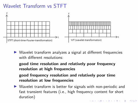
I Wavelet transform analyzes a signal at different frequencieswith different resolutions:
good time resolution and relatively poor frequencyresolution at high frequencies
good frequency resolution and relatively poor timeresolution at low frequencies
I Wavelet transform is better for signals with non-periodic andfast transient features (i.e., high frequency content for shortduration)
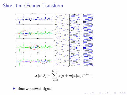
Short-time Fourier Transform
X[n, λ] =
L−1∑m=0
x[n+m]w[m]e−jλm,
I time-windowed signal
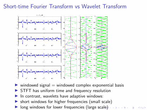
Short-time Fourier Transform vs Wavelet Transform
I windowed signal = windowed complex exponential basisI STFT has uniform time and frequency resolutionI In contrast, wavelets have adaptive windows:I short windows for higher frequencies (small scale)I long windows for lower frequencies (large scale)
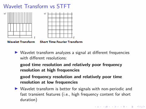
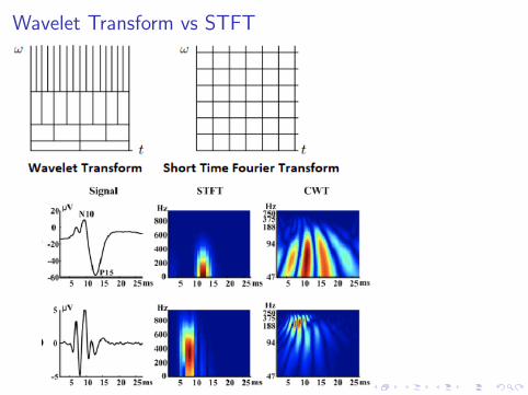
Wavelet Transform vs STFT
I Wavelet transform analyzes a signal at different frequencieswith different resolutions:
good time resolution and relatively poor frequencyresolution at high frequencies
good frequency resolution and relatively poor timeresolution at low frequencies
I Wavelet transform is better for signals with non-periodic andfast transient features (i.e., high frequency content for shortduration)
Wavelet Transform vs STFT
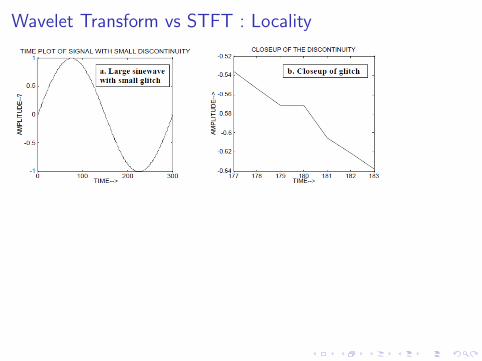
Wavelet Transform vs STFT : Locality
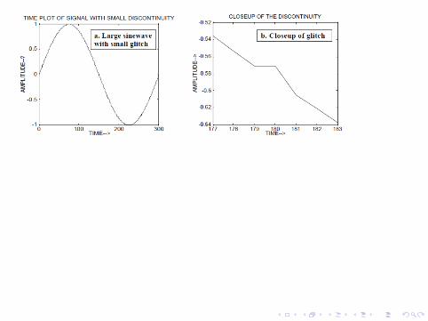
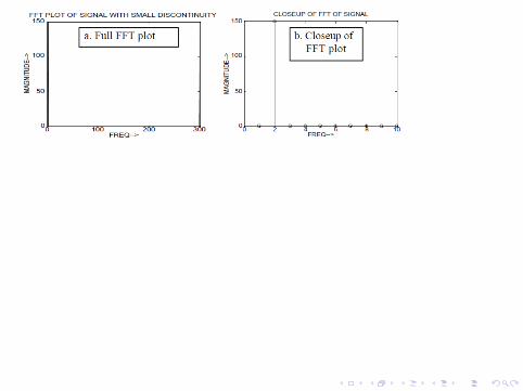
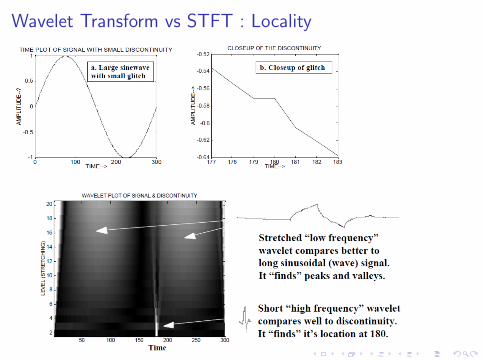
Wavelet Transform vs STFT : Locality
Fourier vs Wavelet Transforms
I Fourier Transform has convolution theorem and mathematicalrelationships
I No closed form relations exist for wavelet transforms
I Fourier transform has uniform spectral resolution
I Wavelet transform has adaptive resolution
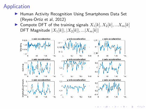
ApplicationI Human Activity Recognition Using Smartphones Data Set
(Reyes-Ortiz et al, 2012)I Compote DFT of the training signals X1[k], X2[k], ...Xm[k]
DFT Magnitude |X1[k]|, |X2[k]|, ...|Xm[k]|
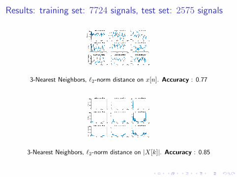
Results: training set: 7724 signals, test set: 2575 signals
3-Nearest Neighbors, `2-norm distance on x[n]. Accuracy : 0.77
3-Nearest Neighbors, `2-norm distance on |X[k]|. Accuracy : 0.85
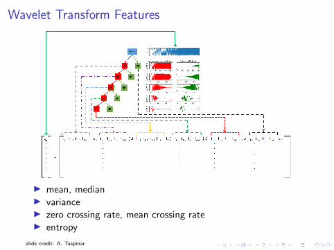
Wavelet Transform Features
I mean, medianI varianceI zero crossing rate, mean crossing rateI entropy
slide credit: A. Taspinar
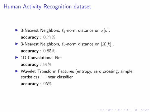
Human Activity Recognition dataset
I 3-Nearest Neighbors, `2-norm distance on x[n].
accuracy : 0.77%
I 3-Nearest Neighbors, `2-norm distance on |X[k]|.accuracy : 0.85%
I 1D Convolutional Net
accuracy : 91%
I Wavelet Transform Features (entropy, zero crossing, simplestatistics) + linear classifier
accuracy : 95%
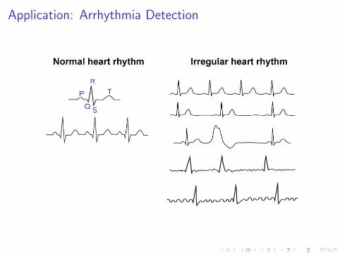
Application: Arrhythmia Detection
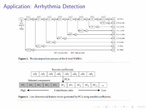
Application: Arrhythmia Detection
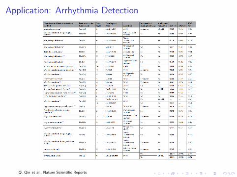
Application: Arrhythmia Detection
Q. Qin et al., Nature Scientific Reports