Lecture 15: Examples of hypothesis tests (v3) Ramesh...

MS&E 226: “Small” DataLecture 15: Examples of hypothesis tests (v3)

Ramesh [email protected]

1 / 31

The recipe

2 / 31

The hypothesis testing recipe

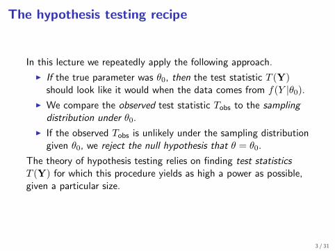
In this lecture we repeatedly apply the following approach.

I If the true parameter was θ0, then the test statistic T (Y)should look like it would when the data comes from f(Y |θ0).

I We compare the observed test statistic Tobs to the samplingdistribution under θ0.

I If the observed Tobs is unlikely under the sampling distributiongiven θ0, we reject the null hypothesis that θ = θ0.

The theory of hypothesis testing relies on finding test statisticsT (Y) for which this procedure yields as high a power as possible,given a particular size.

3 / 31

The Wald test

4 / 31

Assumption: Asymptotic normality

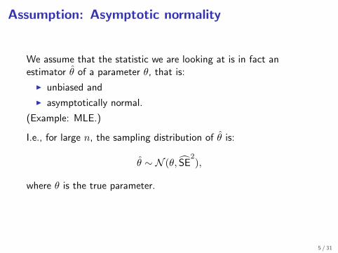
We assume that the statistic we are looking at is in fact anestimator θ of a parameter θ, that is:

I unbiased and

I asymptotically normal.

(Example: MLE.)

I.e., for large n, the sampling distribution of θ is:

θ ∼ N (θ, SE2),

where θ is the true parameter.

5 / 31

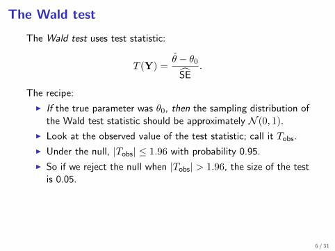
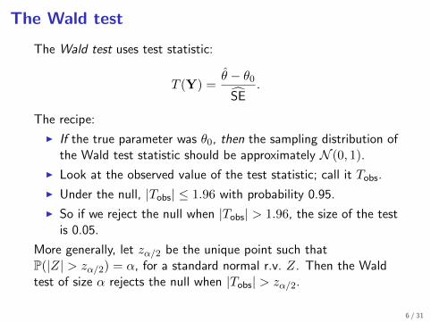
The Wald test

The Wald test uses test statistic:

T (Y) =θ − θ0

SE.

The recipe:

I If the true parameter was θ0, then the sampling distribution ofthe Wald test statistic should be approximately N (0, 1).

I Look at the observed value of the test statistic; call it Tobs.

I Under the null, |Tobs| ≤ 1.96 with probability 0.95.

I So if we reject the null when |Tobs| > 1.96, the size of the testis 0.05.

More generally, let zα/2 be the unique point such thatP(|Z| > zα/2) = α, for a standard normal r.v. Z. Then the Waldtest of size α rejects the null when |Tobs| > zα/2.

6 / 31

The Wald test: A picture

7 / 31

The Wald test and confidence intervals

Recall that a (asymptotic) 1− α confidence interval for the true θis:

[θ − zα/2SE, θ + zα/2SE].

The Wald test is equivalent to rejecting the null if θ0 is not in the1− α confidence interval.

8 / 31

Power of the Wald test

Now suppose the true θ 6= θ0. What is the chance we (correctly)reject the null?

Note that in this case, the sampling distribution of the Wald teststatistic is still approximately normal with variance 1, but now withmean (θ − θ0)/SE.

Therefore the power at θ is approximately P(|Z| > zα/2), where:

Z ∼ N(θ − θ0

SE, 1

).

9 / 31

Power of the Wald test: A picture

10 / 31

Example: Significance of an OLS coefficient

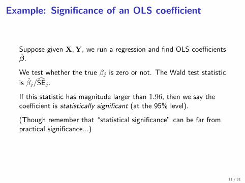
Suppose given X,Y, we run a regression and find OLS coefficientsβ.

We test whether the true βj is zero or not. The Wald test statistic

is βj/SEj .

If this statistic has magnitude larger than 1.96, then we say thecoefficient is statistically significant (at the 95% level).

(Though remember that “statistical significance” can be far frompractical significance...)

11 / 31

p-values

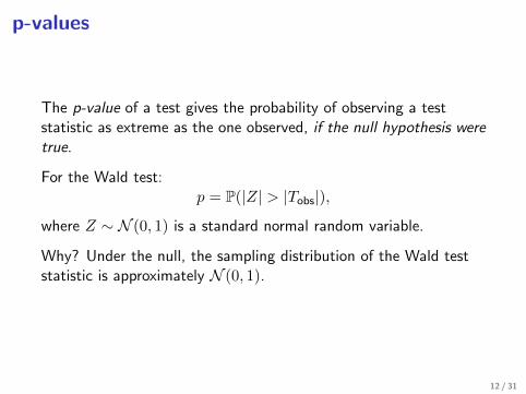
The p-value of a test gives the probability of observing a teststatistic as extreme as the one observed, if the null hypothesis weretrue.

For the Wald test:p = P(|Z| > |Tobs|),

where Z ∼ N (0, 1) is a standard normal random variable.

Why? Under the null, the sampling distribution of the Wald teststatistic is approximately N (0, 1).

12 / 31

p-values

Note that:

I If the p-value is small, the observed test statistic is veryunlikely under the null hypothesis.

I In fact, suppose we reject when p < α. This is exactly thesame as rejecting when |Tobs| > zα/2.

I In other words: The Wald test of size α is obtained byrejecting when the p-value is below α.

13 / 31

p-values: A picture

14 / 31

The sampling distribution of p-values: A picture

15 / 31

Use and misuse of p-values

Why p-values? They are transparent:

I Reporting “statistically significant” (or not) depends on yourchosen value of α.

I What if my desired α is different (more or less conservative)?

I p-values allow different people to interpret the data usingtheir own desired α.

But note: the p-value is not the probability the null hypothesis istrue!

16 / 31

The t-test

17 / 31

The z-test

We assume that Y = (Y1, . . . , Yn) are i.i.d. N (θ, σ2) randomvariables.

If we know σ2:

I The variance of the sampling distribution of Y is σ2/n, so itsexact standard error is SE = σ/

√n.

I Thus if θ = θ0, then (Y − θ0)/SE should be N (0, 1).

I So we can use (Y − θ0)/SE as a test statistic, and proceed aswe did for the Wald statistic. This is called a z-test.

The only difference from the Wald test is that if we know the Yi’sare normally distributed, then the test statistic is exactly normaleven in finite samples.

18 / 31

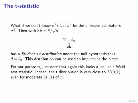
The t-statistic

What if we don’t know σ2? Let σ2 be the unbiased estimator ofσ2. Then with SE = σ/

√n,

Y − θ0SE

has a Student’s t distribution under the null hypothesis thatθ = θ0. This distribution can be used to implement the t-test.

For our purposes, just note that again this looks a lot like a Waldtest statistic! Indeed, the t distribution is very close to N (0, 1),even for moderate values of n.

19 / 31

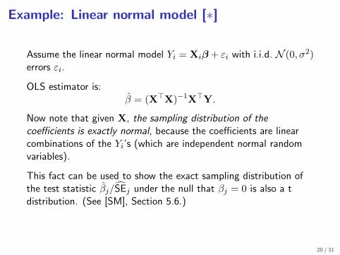
Example: Linear normal model [∗]

Assume the linear normal model Yi = Xiβ+ εi with i.i.d. N (0, σ2)errors εi.

OLS estimator is:β = (X>X)−1X>Y.

Now note that given X, the sampling distribution of thecoefficients is exactly normal, because the coefficients are linearcombinations of the Yi’s (which are independent normal randomvariables).

This fact can be used to show the exact sampling distribution ofthe test statistic βj/SEj under the null that βj = 0 is also a tdistribution. (See [SM], Section 5.6.)

20 / 31

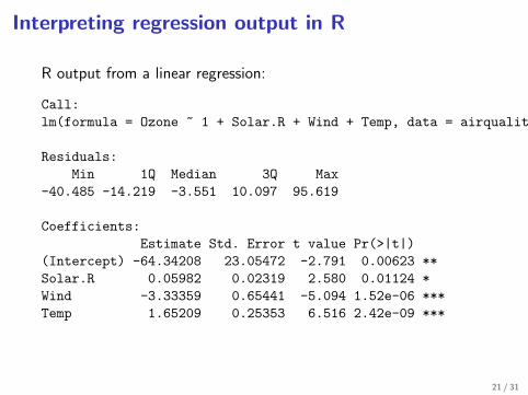
Interpreting regression output in R

R output from a linear regression:

Call:

lm(formula = Ozone ~ 1 + Solar.R + Wind + Temp, data = airquality)

Residuals:

Min 1Q Median 3Q Max

-40.485 -14.219 -3.551 10.097 95.619

Coefficients:

Estimate Std. Error t value Pr(>|t|)

(Intercept) -64.34208 23.05472 -2.791 0.00623 **

Solar.R 0.05982 0.02319 2.580 0.01124 *

Wind -3.33359 0.65441 -5.094 1.52e-06 ***

Temp 1.65209 0.25353 6.516 2.42e-09 ***

21 / 31

Statistical significance in R

In most statistical software (and in papers), statistical significanceis denoted as follows:

I *** means “statistically significant at the 99.9% level”.

I ** means “statistically significant at the 99% level”.

I * means “statistically significant at the 95% level”.

22 / 31

The F test in linear regression

23 / 31

Multiple regression coefficients

We again assume we are in the linear normal model:Yi = Xiβ + εi with i.i.d. N (0, σ2) errors εi.

The Wald (or t) test lets us test whether one regression coefficientis zero.

What if we want to know if multiple regression coefficients arezero? This is equivalent to asking: would a simpler model suffice?For this purpose we use the F test.

24 / 31

The F statistic

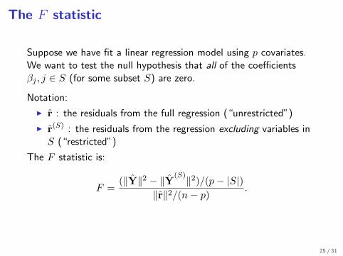
Suppose we have fit a linear regression model using p covariates.We want to test the null hypothesis that all of the coefficientsβj , j ∈ S (for some subset S) are zero.

Notation:

I r : the residuals from the full regression (“unrestricted”)

I r(S) : the residuals from the regression excluding variables inS (“restricted”)

The F statistic is:

F =(‖Y‖2 − ‖Y(S)‖2)/(p− |S|)

‖r‖2/(n− p).

25 / 31

The F test

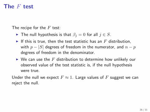
The recipe for the F test:

I The null hypothesis is that βj = 0 for all j ∈ S.

I If this is true, then the test statistic has an F distribution,with p− |S| degrees of freedom in the numerator, and n− pdegrees of freedom in the denominator.

I We can use the F distribution to determine how unlikely ourobserved value of the test statistic is, if the null hypothesiswere true.

Under the null we expect F ≈ 1. Large values of F suggest we canreject the null.

26 / 31

The F test

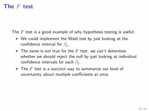
The F test is a good example of why hypothesis testing is useful:

I We could implement the Wald test by just looking at theconfidence interval for βj .

I The same is not true for the F test: we can’t determinewhether we should reject the null by just looking at individualconfidence intervals for each βj .

I The F test is a succinct way to summarize our level ofuncertainty about multiple coefficients at once.

27 / 31

“The” F test

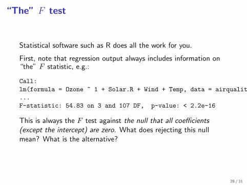
Statistical software such as R does all the work for you.

First, note that regression output always includes information on“the” F statistic, e.g.:

Call:

lm(formula = Ozone ~ 1 + Solar.R + Wind + Temp, data = airquality)

...

F-statistic: 54.83 on 3 and 107 DF, p-value: < 2.2e-16

This is always the F test against the null that all coefficients(except the intercept) are zero. What does rejecting this nullmean? What is the alternative?

28 / 31

F tests of one model against another

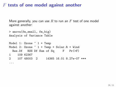
More generally, you can use R to run an F test of one modelagainst another:

> anova(fm_small, fm_big)

Analysis of Variance Table

Model 1: Ozone ~ 1 + Temp

Model 2: Ozone ~ 1 + Temp + Solar.R + Wind

Res.Df RSS Df Sum of Sq F Pr(>F)

1 109 62367

2 107 48003 2 14365 16.01 8.27e-07 ***

...

29 / 31

Caution

30 / 31

A word of warning

Used correctly, hypothesis tests are powerful tools to quantify youruncertainty.

However, they can easily be misused, as we will see later in thecourse. Some questions for thought:

I Suppose with 1000 covariates, you use the t (or Wald)statistic on each coefficient to determine whether to includeor exclude it. What might go wrong?

I Suppose that you test and compare many models byrepeatedly using F tests. What might go wrong?

31 / 31

Lecture 15: Examples of hypothesis tests (v3) Ramesh...

Documents

Transcript of Lecture 15: Examples of hypothesis tests (v3) Ramesh...