
Lecture 13 Auto/cross-correlation - Bauer College of … · 1 1 Lecture 13 Auto/cross-correlation...
24
RS – Lecture 13 1 1 Lecture 13 Auto/cross-correlation • The generalized regression model's assumptions: (A1) DGP: y = X + is correctly specified. (A2) E[|X] = 0 (A3’) Var[|X] = Σ = 2 . (A4) X has full column rank – rank(X)=k-, where T ≥ k. • We assume that the ’s in the sample are not longer generated independently of each other. Ignoring hetersocedasticity, we have a new Σ: E[ i j |X] = ij if i ≠j = 2 if i=j Generalized Regression Model
Transcript of Lecture 13 Auto/cross-correlation - Bauer College of … · 1 1 Lecture 13 Auto/cross-correlation...
RS – Lecture 13
1
1
Lecture 13Auto/cross-correlation
• The generalized regression model's assumptions:
(A1) DGP: y = X + is correctly specified.
(A2) E[|X] = 0
(A3’) Var[|X] = Σ = 2.
(A4) X has full column rank – rank(X)=k-, where T ≥ k.
• We assume that the ’s in the sample are not longer generated independently of each other. Ignoring hetersocedasticity, we have a new Σ:
E[ij|X] = ij if i ≠j
= 2 if i=j
Generalized Regression Model
RS – Lecture 13
2
• We keep the linear model:
- First-order autoregressive autocorrelation: AR(1)
- Fifth-order autoregressive autocorrelation: AR(5)
- Third-order moving average autocorrelation: MA(3)
ttt u 1
ttttttt u 5544332211
332211 ttttt uuuu
8
Note: The last example is described as third-order moving average autocorrelation, denoted MA(3), because it depends on the three previous innovations as well as the current one.
ttt Xy '
Autocorrelation: Examples
Implications for OLS
• Similar to the heteroscedasticity results: - OLS is unbiased, consistent (we need additional assumptions), asymptotic normality (we need additional assumptions and definitions), but inefficient. - OLS standard errors are incorrect, often biased downwards.
• A very important exception: The lagged dependent variableyt = xt + yt-1 + t. t = t-1 + ut.
Now, Cov[yt-1 ,t ] 0 ⟹ IV Estimation
• Useful strategy: OLS estimates with the Newey-West (NW) robust estimation of the covariance matrix. Recall NW’s HAC estimator of Q*:
ST = S0 + (1/T) l wL(l) t=l+1,...,T (xt-let-l etxt+ xtet et-lxt-l)
RS – Lecture 13
3
Newey-West estimator
• The performance of NW estimators depends on the choice of the kernel function –i.e., wL– and truncation lag (L). These choices affect the resulting test statistics and render testing results fragile.
• NW SEs perform poorly in Monte Carlo simulations: the finite-sample performance of tests using NW SE is not well approximated by the asymptotic theory (big size problems), especially when show xtet moderate or high persistence:
- The kernel weighting scheme yields negative bias –i.e., NW SEs are downward biased–, which could be big in finite samples.
- The tests based on the NW SE usually over-reject H0.
- A relatively small L is needed to minimize MSE, which leads to considerable bias of the Q* estimator (&, then, distorts the size the tests). Minimizing size distortions needs a larger L.
Newey-West estimator: Implementation
• To implement the HAC estimator, we need to determine: lag order –i.e., truncation lag (L) or bandwidth–, and kernel choice (wl (L)).
(1) Truncation lag (L) No optimal formula; though selecting L to minimize MSE is popular.
To determine L, we use: - Trial and error, informed guess.- Rules of thumb. For example: L+1 = 0.75T1/3.- Automatic selection rules, following Andrews (1991), Newey
and West (1994) or Sun et al. (2008).
The choice of L matters. In general, for ARMA models we have: - Shorter lags: Larger Bias, Smaller Variance- Longer lags: Smaller Bias, Larger Variance
RS – Lecture 13
4
Newey-West estimator: Implementation
• The usual practical advise regarding lags: Choose lags a little longer than you might otherwise.
• Sun et al. (2008) give some intuition using for longer lags than the MSE Optimal, by expanding the probability of a test. Simple example:
Let z~N(0, σ2), s2 is an estimator of σ2 (assume independent of z).
)('g'MSE2
1)(g')Bias()(
)('g')(2
1)(g')g(
)g(][IPrPr
2222
22222222
222222
2
21
sscF
sEsEE
sEcszEcszcs
z
⟹ Equal weight MSE + Bias. Longer L minimize the Bias; better size!
Newey-West estimator: Implementation
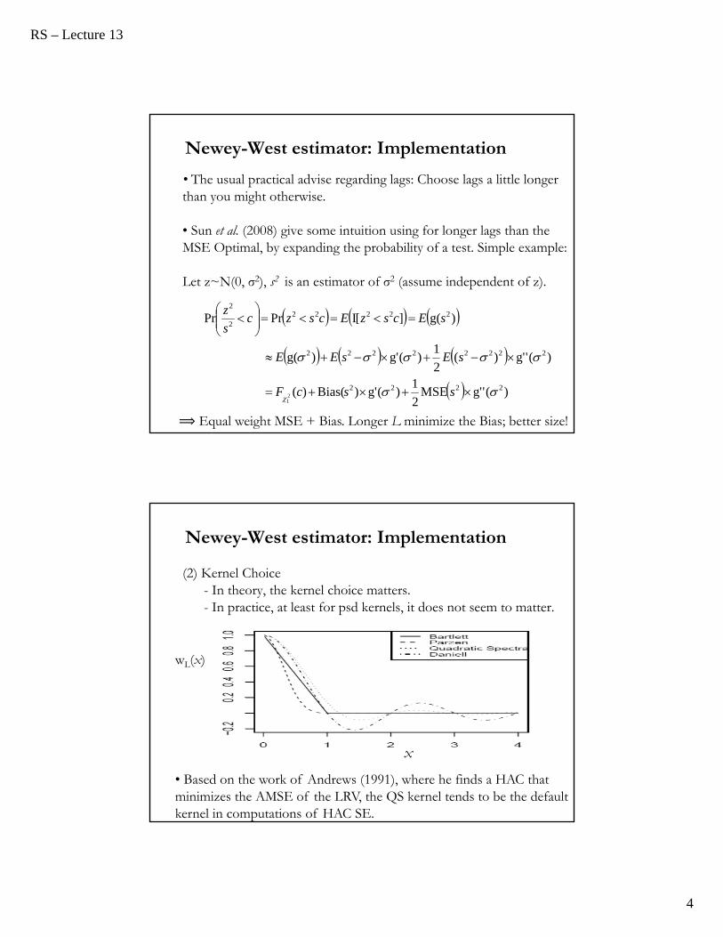
(2) Kernel Choice- In theory, the kernel choice matters.- In practice, at least for psd kernels, it does not seem to matter.
wL(x)
x
• Based on the work of Andrews (1991), where he finds a HAC that minimizes the AMSE of the LRV, the QS kernel tends to be the default kernel in computations of HAC SE.
RS – Lecture 13
5
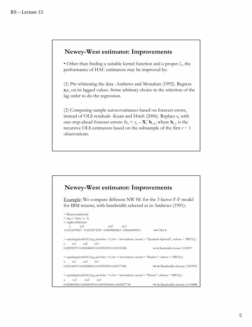
Newey-West estimator: Improvements
• Other than finding a suitable kernel function and a proper L, the performance of HAC estimators may be improved by:
(1) Pre-whitening the data -Andrews and Monahan (1992). Regress xiet on its lagged values. Some arbitrary choice in the selection of the lag order to do the regression.
(2) Computing sample autocovariances based on forecast errors, instead of OLS residuals -Kuan and Hsieh (2006). Replace et with one-step-ahead forecast errors: fet = yt – Xt’ bt-1, where bt-1 is the recursive OLS estimators based on the subsample of the first t − 1 observations.
Newey-West estimator: Improvements
Example: We compute different NW SE for the 3 factor F-F model for IBM returns, with bandwidth selected as in Andrews (1991):
> library(sandwich)> reg <- lm(y~x -1)> reg$coefficients
x xx1 xx2 xx3 -0.2331470817 0.0101872239 0.0009802843 -0.0044459013 ⟹ OLS b
> sqrt(diag(kernHAC(reg, prewhite = 0, bw = bwAndrews, kernel = "Quadratic Spectral", verbose = TRUE)))
x xx1 xx2 xx3
0.020959375 0.002848645 0.003983330 0.005310548 ⟹ & Bandwidth chosen: 3.035697
> sqrt(diag(kernHAC(reg, prewhite = 0, bw = bwAndrews, kernel = "Bartlett", verbose = TRUE)))
x xx1 xx2 xx3
0.020344074 0.002828663 0.003995942 0.005177482 ⟹ & Bandwidth chosen: 3.507051
> sqrt(diag(kernHAC(reg, prewhite = 0, bw = bwAndrews, kernel = "Parzen", verbose = TRUE)))
x xx1 xx2 xx3
0.022849506 0.002839034 0.003954436 0.005427730 ⟹ & Bandwidth chosen: 6.110888
RS – Lecture 13
6
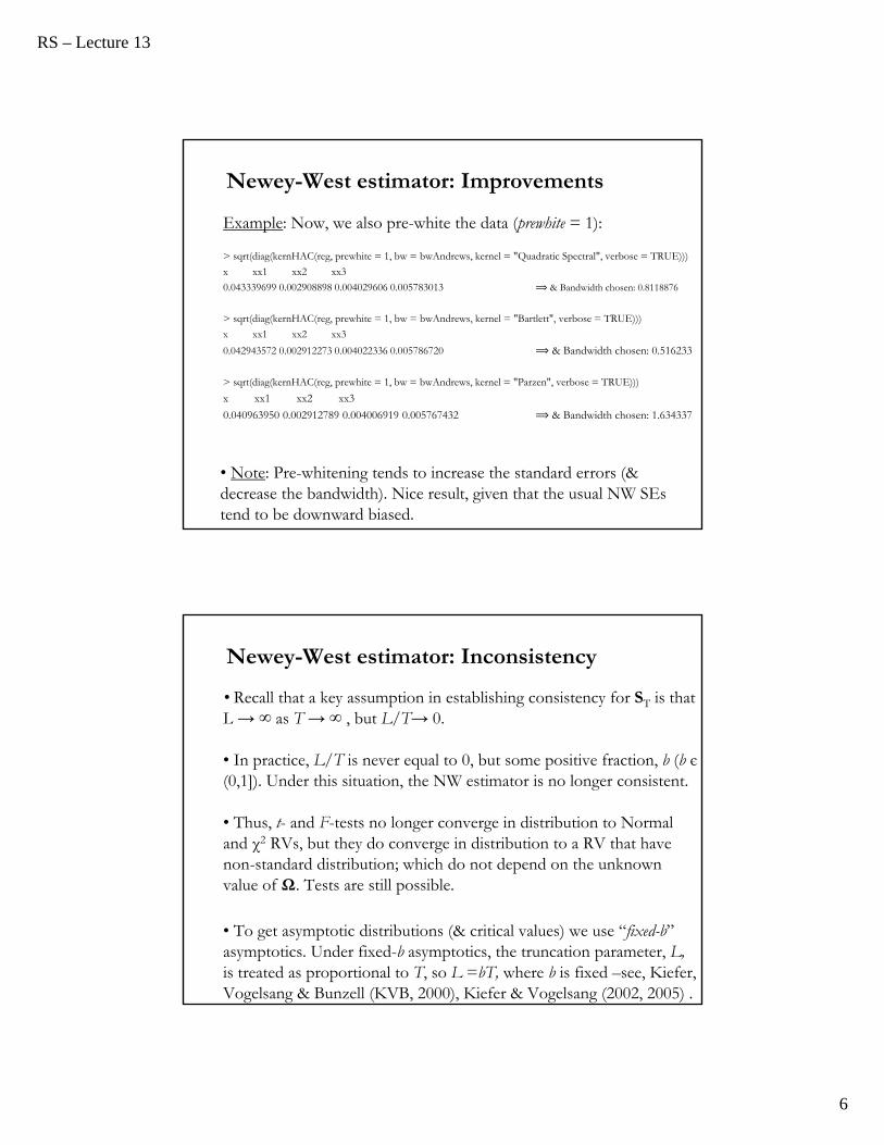
Newey-West estimator: Improvements
Example: Now, we also pre-white the data (prewhite = 1):
> sqrt(diag(kernHAC(reg, prewhite = 1, bw = bwAndrews, kernel = "Quadratic Spectral", verbose = TRUE)))
x xx1 xx2 xx3
0.043339699 0.002908898 0.004029606 0.005783013 ⟹ & Bandwidth chosen: 0.8118876
> sqrt(diag(kernHAC(reg, prewhite = 1, bw = bwAndrews, kernel = "Bartlett", verbose = TRUE)))
x xx1 xx2 xx3
0.042943572 0.002912273 0.004022336 0.005786720 ⟹ & Bandwidth chosen: 0.516233
> sqrt(diag(kernHAC(reg, prewhite = 1, bw = bwAndrews, kernel = "Parzen", verbose = TRUE)))
x xx1 xx2 xx3
0.040963950 0.002912789 0.004006919 0.005767432 ⟹ & Bandwidth chosen: 1.634337
• Note: Pre-whitening tends to increase the standard errors (& decrease the bandwidth). Nice result, given that the usual NW SEs tend to be downward biased.
Newey-West estimator: Inconsistency
• Recall that a key assumption in establishing consistency for ST is that L → ∞ as T → ∞ , but L/T→ 0.
• In practice, L/T is never equal to 0, but some positive fraction, b (b є(0,1]). Under this situation, the NW estimator is no longer consistent.
• Thus, t- and F-tests no longer converge in distribution to Normal and χ2 RVs, but they do converge in distribution to a RV that have non-standard distribution; which do not depend on the unknown value of Ω. Tests are still possible.
• To get asymptotic distributions (& critical values) we use “fixed-b” asymptotics. Under fixed-b asymptotics, the truncation parameter, L,is treated as proportional to T, so L =bT, where b is fixed –see, Kiefer, Vogelsang & Bunzell (KVB, 2000), Kiefer & Vogelsang (2002, 2005) .
RS – Lecture 13
7
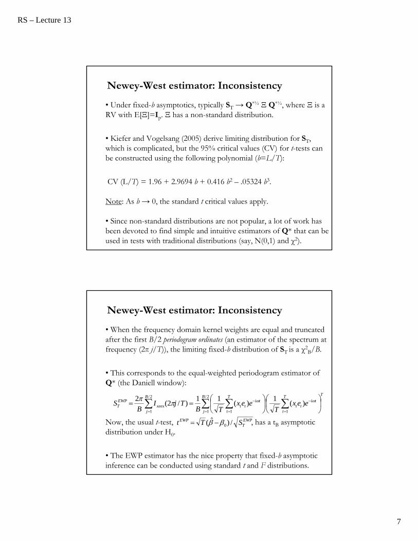
Newey-West estimator: Inconsistency
• Under fixed-b asymptotics, typically ST → Q*½ Ξ Q*½, where Ξ is a RV with E[Ξ]=Ip. Ξ has a non-standard distribution.
• Kiefer and Vogelsang (2005) derive limiting distribution for ST, which is complicated, but the 95% critical values (CV) for t-tests can be constructed using the following polynomial (b=L/T):
CV (L/T) = 1.96 + 2.9694 b + 0.416 b2 – .05324 b3.
Note: As b → 0, the standard t critical values apply.
• Since non-standard distributions are not popular, a lot of work has been devoted to find simple and intuitive estimators of Q* that can be used in tests with traditional distributions (say, N(0,1) and χ2).
Newey-West estimator: Inconsistency
• When the frequency domain kernel weights are equal and truncated after the first B/2 periodogram ordinates (an estimator of the spectrum at frequency (2π j/T)), the limiting fixed-b distribution of ST is a χ2
B/B.
• This corresponds to the equal-weighted periodogram estimator of Q* (the Daniell window):
Now, the usual t-test, , has a tB asymptotic distribution under H0.
• The EWP estimator has the nice property that fixed-b asymptotic inference can be conducted using standard t and F distributions.
TT
t
titt
B
j
T
t
titt
B
jxeex
EWPT eex
Teex
TBTjI
BS
1
2/
1 1
2/
1
)(1
)(11
)/2(2
EWPT
EWP STt /)ˆ( 0
RS – Lecture 13
8
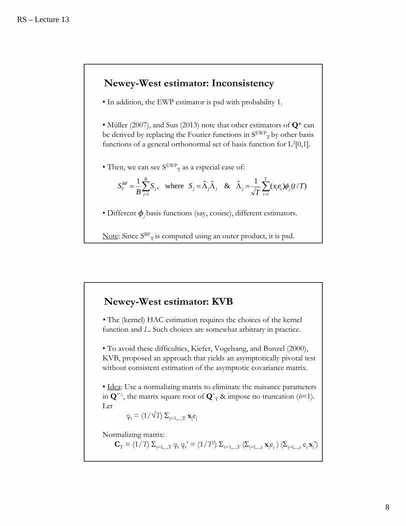
Newey-West estimator: Inconsistency
• In addition, the EWP estimator is psd with probability 1.
• Müller (2007), and Sun (2013) note that other estimators of Q* can be derived by replacing the Fourier functions in SEWP
T by other basis functions of a general orthonormal set of basis function for L2[0,1].
• Then, we can see SEWPT as a especial case of:
• Different j basis functions (say, cosine), different estimators.
Note: Since SBFT is computed using an outer product, it is psd.
T
tjtt
B
jjjjjj
BFT Ttex
TSS
BS
11
' )/()(1ˆ&ˆˆwhere,
1
Newey-West estimator: KVB
• The (kernel) HAC estimation requires the choices of the kernel function and L. Such choices are somewhat arbitrary in practice.
• To avoid these difficulties, Kiefer, Vogelsang, and Bunzel (2000), KVB, proposed an approach that yields an asymptotically pivotal test without consistent estimation of the asymptotic covariance matrix.
• Idea: Use a normalizing matrix to eliminate the nuisance parameters in Q*½, the matrix square root of Q*
T & impose no truncation (b=1). Let
φt = (1/√T) j=1,...,T xjej
Normalizing matrix:CT = (1/T) t=l,...,T φt φt’ = (1/T2) t=1,...,T (j=l,...,t xjej ) (j=l,...,t ej xj’)
RS – Lecture 13
9
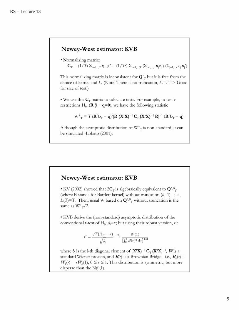
Newey-West estimator: KVB
• Normalizing matrix:CT = (1/T) t=l,...,T φt φt’ = (1/T2) t=1,...,T (j=l,...,t xjej ) (j=l,...,t ej xj’)
This normalizing matrix is inconsistent for Q*T but it is free from the
choice of kernel and L. (Note: There is no truncation, L=T => Good for size of test!)
• We use this CT matrix to calculate tests. For example, to test r restrictions H0: (R β− q=0), we have the following statistic
W+T = T (RˆbT− q)’[R (X’X)−1 CT (X’X)−1 R] -1 (RˆbT− q).
Although the asymptotic distribution of W+T is non-standard, it can
be simulated -Lobato (2001).
Newey-West estimator: KVB
• KV (2002) showed that 2CT is algebraically equivalent to Q*,BT
(where B stands for Bartlett kernel) without truncation (b=1) - i.e., L(T)=T. Then, usual W based on Q*,B
T without truncation is the same as W+
T/2.
• KVB derive the (non-standard) asymptotic distribution of the conventional t-test of H0: βi=r ; but using their robust version, t+:
where δi is the i-th diagonal element of (X’X)−1 CT (X’X)−1, W is a standard Wiener process, and B(r) is a Brownian Bridge –i.e., Bk(r) = Wk(r) − rWk(1), 0 ≤ r ≤ 1. This distribution is symmetric, but more disperse than the N(0,1).
RS – Lecture 13
10
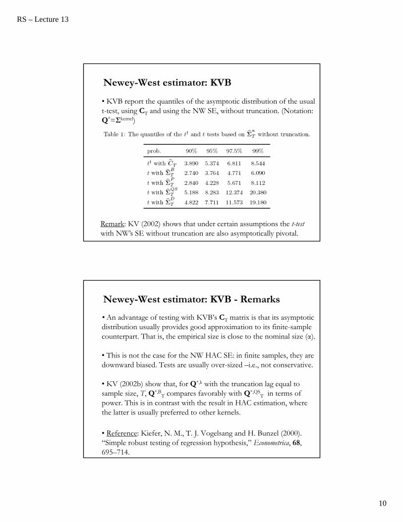
Newey-West estimator: KVB
• KVB report the quantiles of the asymptotic distribution of the usual t-test, using CT and using the NW SE, without truncation. (Notation: Q*=Σkernel)
Remark: KV (2002) shows that under certain assumptions the t-testwith NW’s SE without truncation are also asymptotically pivotal.
Newey-West estimator: KVB - Remarks
• An advantage of testing with KVB’s CT matrix is that its asymptotic distribution usually provides good approximation to its finite-sample counterpart. That is, the empirical size is close to the nominal size (α).
• This is not the case for the NW HAC SE: in finite samples, they are downward biased. Tests are usually over-sized –i.e., not conservative.
• KV (2002b) show that, for Q*,k with the truncation lag equal to sample size, T, Q*,B
T compares favorably with Q*,QST in terms of
power. This is in contrast with the result in HAC estimation, where the latter is usually preferred to other kernels.
• Reference: Kiefer, N. M., T. J. Vogelsang and H. Bunzel (2000). “Simple robust testing of regression hypothesis,” Econometrica, 68, 695–714.
RS – Lecture 13
11
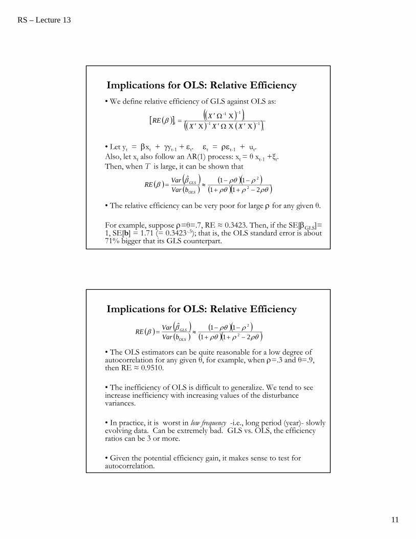
Implications for OLS: Relative Efficiency
• We define relative efficiency of GLS against OLS as:
• Let yt = xt + yt-1 + t. t = t-1 + ut. Also, let xt also follow an AR(1) process: xt = θ xt-1 +ξt.Then, when T is large, it can be shown that
• The relative efficiency can be very poor for large for any given θ.
For example, suppose =θ=.7, RE ≈ 0.3423. Then, if the SE[GLS]= 1, SE[b] = 1.71 (= 0.3423-.5); that is, the OLS standard error is about 71% bigger that its GLS counterpart.
i
ii
XXX
XRE 11
11-
X X X
X
211
11ˆ2
2
OLS
GLS
bVar
VarRE
Implications for OLS: Relative Efficiency
• The OLS estimators can be quite reasonable for a low degree of autocorrelation for any given θ, for example, when =.3 and θ=.9,then RE ≈ 0.9510.
• The inefficiency of OLS is difficult to generalize. We tend to see increase inefficiency with increasing values of the disturbance variances.
• In practice, it is worst in low frequency -i.e., long period (year)- slowly evolving data. Can be extremely bad. GLS vs. OLS, the efficiency ratios can be 3 or more.
• Given the potential efficiency gain, it makes sense to test for autocorrelation.
211
11ˆ2
2
OLS
GLS
bVar
VarRE
RS – Lecture 13
12
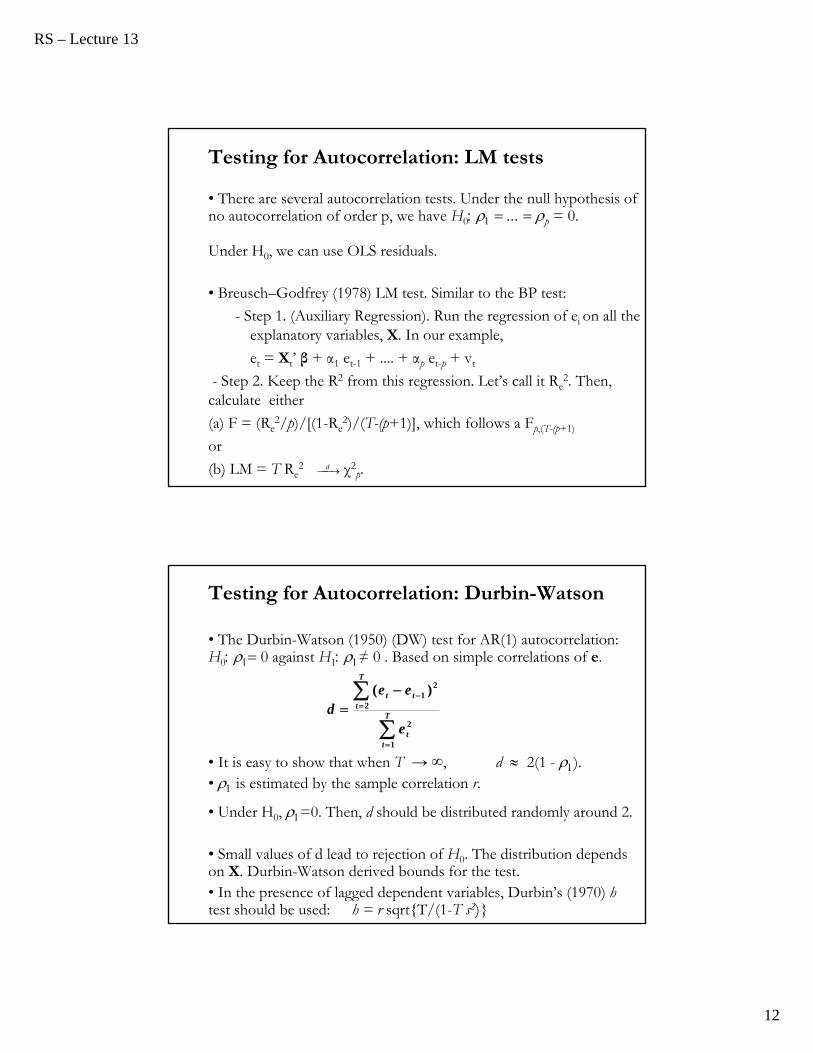
Testing for Autocorrelation: LM tests
• There are several autocorrelation tests. Under the null hypothesis of no autocorrelation of order p, we have H0 p = 0.
Under H0, we can use OLS residuals.
• Breusch–Godfrey (1978) LM test. Similar to the BP test:
- Step 1. (Auxiliary Regression). Run the regression of ei on all the explanatory variables, X. In our example,
et = Xt’ β + α1 et-1 + .... + αp et-p + vt
- Step 2. Keep the R2 from this regression. Let’s call it Re2. Then,
calculate either
(a) F = (Re2/p)/[(1-Re
2)/(T-(p+1)], which follows a Fp,(T-(p+1)
or
(b) LM = T Re2 χ2
p.d
Testing for Autocorrelation: Durbin-Watson
• The Durbin-Watson (1950) (DW) test for AR(1) autocorrelation: H00 against H1≠ 0 . Based on simple correlations of e.
• It is easy to show that when T → ∞, d 2(1 - ). • is estimated by the sample correlation r.
• Under H0, =0. Then, d should be distributed randomly around 2.
• Small values of d lead to rejection of H0. The distribution depends on X. Durbin-Watson derived bounds for the test.• In the presence of lagged dependent variables, Durbin’s (1970) h test should be used: h = r sqrtT/(1-T s2)
T
tt
T
ttt
e
eed
1
2
2
21 )(
RS – Lecture 13
13
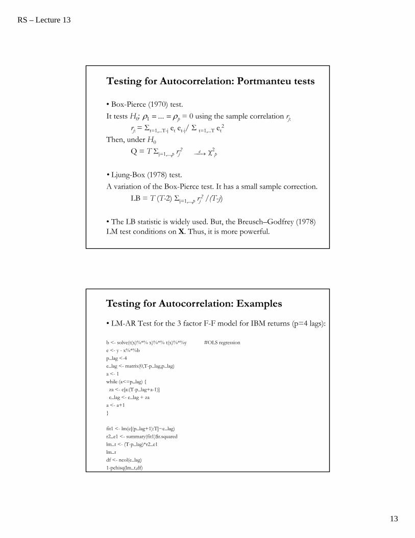
Testing for Autocorrelation: Portmanteu tests
• Box-Pierce (1970) test.
It tests H0 p = 0 using the sample correlation rj:
rj: = Σt=1,...T-j et et-j/ Σ t=1,...T et2
Then, under H0
Q = T Σj=1,...,p rj2 χ2
p
• Ljung-Box (1978) test.
A variation of the Box-Pierce test. It has a small sample correction.
LB = T (T-2) Σj=1,...,p rj2 /(T-j)
• The LB statistic is widely used. But, the Breusch–Godfrey (1978) LM test conditions on X. Thus, it is more powerful.
d
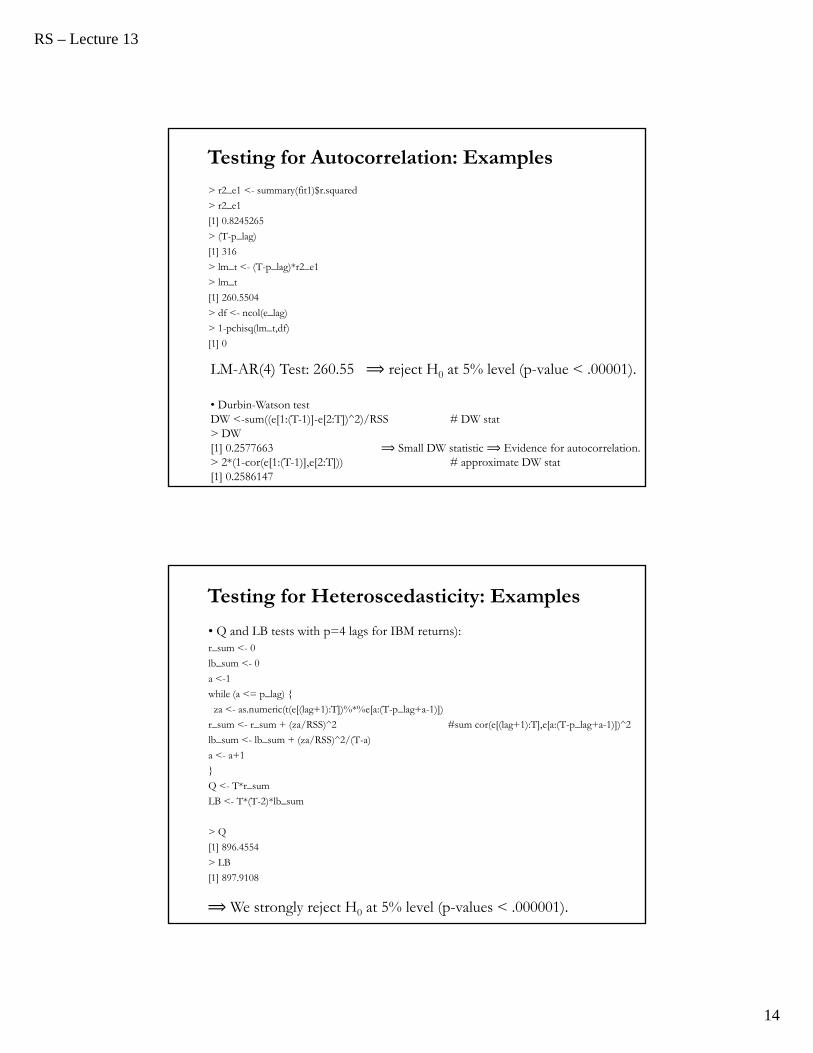
• LM-AR Test for the 3 factor F-F model for IBM returns (p=4 lags):
b <- solve(t(x)%*% x)%*% t(x)%*%y #OLS regression
e <- y - x%*%b
p_lag <-4
e_lag <- matrix(0,T-p_lag,p_lag)
a <- 1
while (a<=p_lag)
za <- e[a:(T-p_lag+a-1)]
e_lag <- e_lag + za
a <- a+1
fit1 <- lm(e[(p_lag+1):T]~e_lag)
r2_e1 <- summary(fit1)$r.squared
lm_t <- (T-p_lag)*r2_e1
lm_t
df <- ncol(e_lag)
1-pchisq(lm_t,df)
Testing for Autocorrelation: Examples
RS – Lecture 13
14
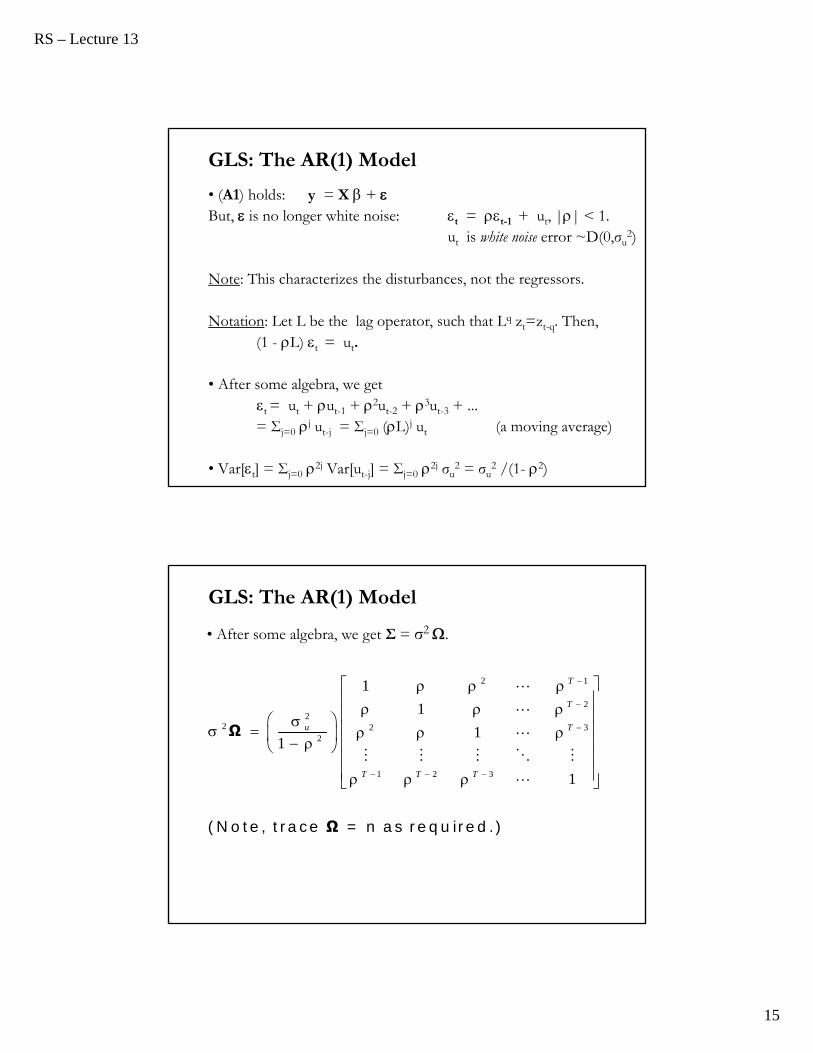
> r2_e1 <- summary(fit1)$r.squared
> r2_e1
[1] 0.8245265
> (T-p_lag)
[1] 316
> lm_t <- (T-p_lag)*r2_e1
> lm_t
[1] 260.5504
> df <- ncol(e_lag)
> 1-pchisq(lm_t,df)
[1] 0
LM-AR(4) Test: 260.55 ⟹ reject H0 at 5% level (p-value < .00001).
• Durbin-Watson testDW <-sum((e[1:(T-1)]-e[2:T])^2)/RSS # DW stat> DW[1] 0.2577663 ⟹ Small DW statistic ⟹ Evidence for autocorrelation.> 2*(1-cor(e[1:(T-1)],e[2:T])) # approximate DW stat[1] 0.2586147
Testing for Autocorrelation: Examples
• Q and LB tests with p=4 lags for IBM returns):r_sum <- 0
lb_sum <- 0
a <-1
while (a <= p_lag)
za <- as.numeric(t(e[(lag+1):T])%*%e[a:(T-p_lag+a-1)])
r_sum <- r_sum + (za/RSS)^2 #sum cor(e[(lag+1):T],e[a:(T-p_lag+a-1)])^2
lb_sum <- lb_sum + (za/RSS)^2/(T-a)
a <- a+1
Q <- T*r_sum
LB <- T*(T-2)*lb_sum
> Q
[1] 896.4554
> LB
[1] 897.9108
⟹ We strongly reject H0 at 5% level (p-values < .000001).
Testing for Heteroscedasticity: Examples
RS – Lecture 13
15
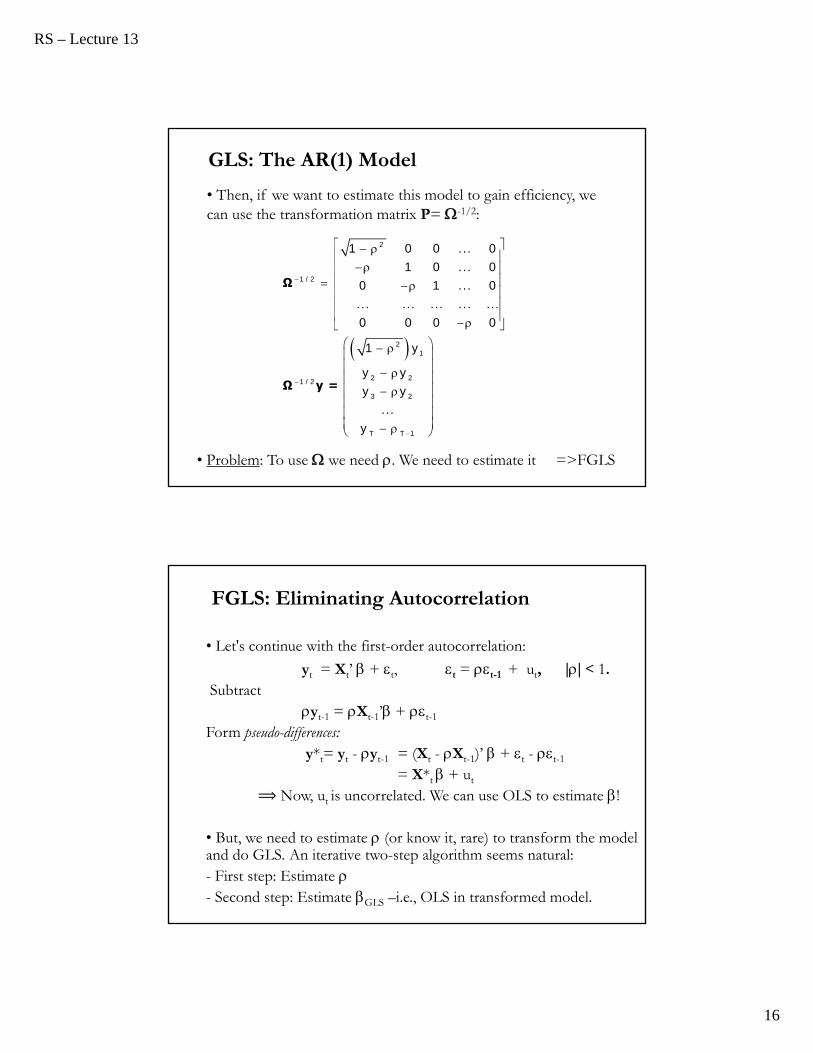
GLS: The AR(1) Model
• (A1) holds: y = X + But, is no longer white noise: t = t-1 + ut, || < 1.
ut is white noise error ~D(0,σu2)
Note: This characterizes the disturbances, not the regressors.
Notation: Let L be the lag operator, such that Lq zt=zt-q. Then, (1 - L) t = ut.
• After some algebra, we gett = ut + ut-1 + 2ut-2 + 3ut-3 + ...= Σj=0 j ut-j = Σj=0 (L)j ut (a moving average)
• Var[t] = Σj=0 2j Var[ut-j] = Σj=0 2j σu2 = σu
2 /(1- 2)
2 1
22
2 2 32
1 2 3
1
1
11
1
( N o te , t r a c e = n a s r e q u ir e d .)
Ω
Ω
T
T
u T
T T T
• After some algebra, we get Σ = σ2 .
GLS: The AR(1) Model
RS – Lecture 13
16
2
1 / 2
21
2 21 / 2
3 2
T T 1
1 0 0 ... 01 0 ... 0
0 1 ... 0... ... ... ... ...0 0 0 0
1 y
y yy y
...y
Ω
Ω y =
• Then, if we want to estimate this model to gain efficiency, we can use the transformation matrix P= -1/2:
• Problem: To use we need . We need to estimate it =>FGLS
GLS: The AR(1) Model
FGLS: Eliminating Autocorrelation
• Let's continue with the first-order autocorrelation:
yt = Xt’ + t, t = t-1 + ut, || < 1.Subtract
yt-1 = Xt-1’ + t-1
Form pseudo-differences:y*t= yt - yt-1 = (Xt - Xt-1)’ + t - t-1
= X*t + ut
⟹ Now, ut is uncorrelated. We can use OLS to estimate !
• But, we need to estimate (or know it, rare) to transform the model and do GLS. An iterative two-step algorithm seems natural: - First step: Estimate - Second step: Estimate GLS –i.e., OLS in transformed model.
RS – Lecture 13
17
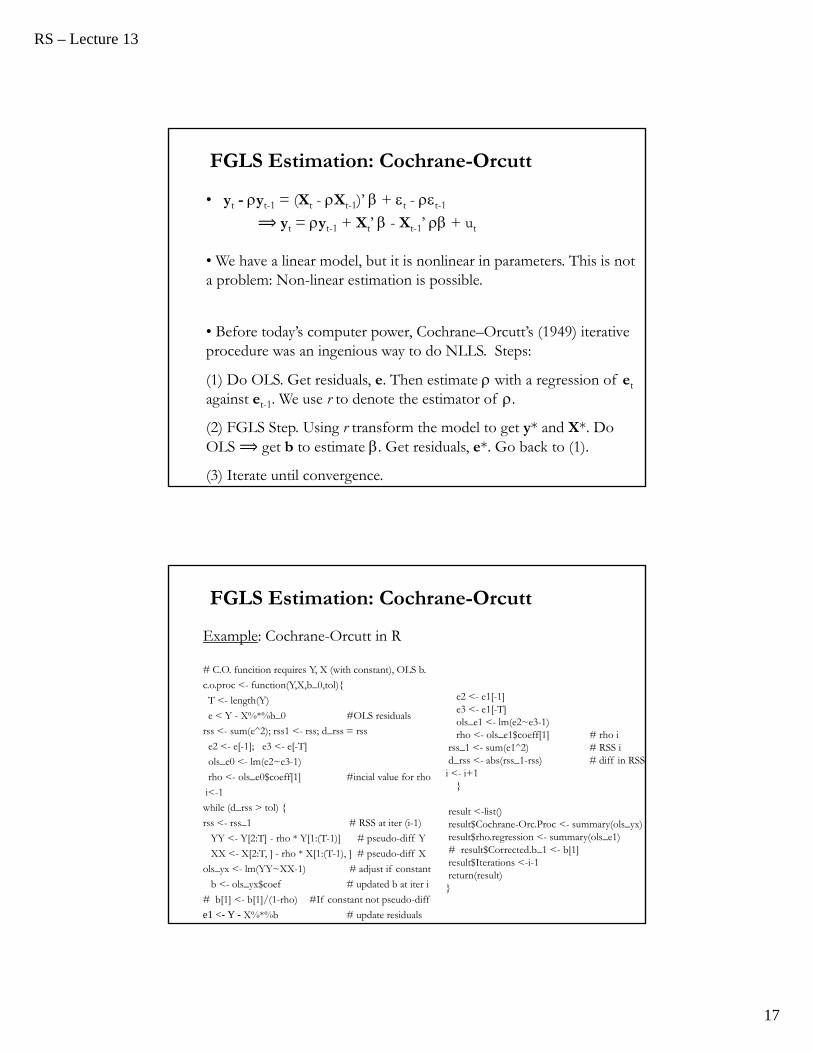
FGLS Estimation: Cochrane-Orcutt
• yt - yt-1 = (Xt - Xt-1)’ + t - t-1
⟹ yt = yt-1 + Xt’ - Xt-1’ + ut
• We have a linear model, but it is nonlinear in parameters. This is not a problem: Non-linear estimation is possible.
• Before today’s computer power, Cochrane–Orcutt’s (1949) iterative procedure was an ingenious way to do NLLS. Steps:
(1) Do OLS. Get residuals, e. Then estimate with a regression of et
against et-1. We use r to denote the estimator of .
(2) FGLS Step. Using r transform the model to get y* and X*. Do OLS ⟹ get b to estimate . Get residuals, e*. Go back to (1).
(3) Iterate until convergence.
Example: Cochrane-Orcutt in R
# C.O. funcition requires Y, X (with constant), OLS b.
c.o.proc <- function(Y,X,b_0,tol)
T <- length(Y)
e < Y - X%*%b_0 #OLS residuals
rss <- sum(e^2); rss1 <- rss; d_rss = rss
e2 <- e[-1]; e3 <- e[-T]
ols_e0 <- lm(e2~e3-1)
rho <- ols_e0$coeff[1] #incial value for rho
i<-1
while (d_rss > tol)
rss <- rss_1 # RSS at iter (i-1)
YY <- Y[2:T] - rho * Y[1:(T-1)] # pseudo-diff Y
XX <- X[2:T, ] - rho * X[1:(T-1), ] # pseudo-diff X
ols_yx <- lm(YY~XX-1) # adjust if constant
b <- ols_yx$coef # updated b at iter i
# b[1] <- b[1]/(1-rho) #If constant not pseudo-diff
e1 <- Y - X%*%b # update residuals
e2 <- e1[-1]e3 <- e1[-T]ols_e1 <- lm(e2~e3-1)rho <- ols_e1$coeff[1] # rho i
rss_1 <- sum(e1^2) # RSS id_rss <- abs(rss_1-rss) # diff in RSSi <- i+1
result <-list()result$Cochrane-Orc.Proc <- summary(ols_yx)result$rho.regression <- summary(ols_e1)# result$Corrected.b_1 <- b[1]result$Iterations <-i-1return(result)
FGLS Estimation: Cochrane-Orcutt
RS – Lecture 13
18
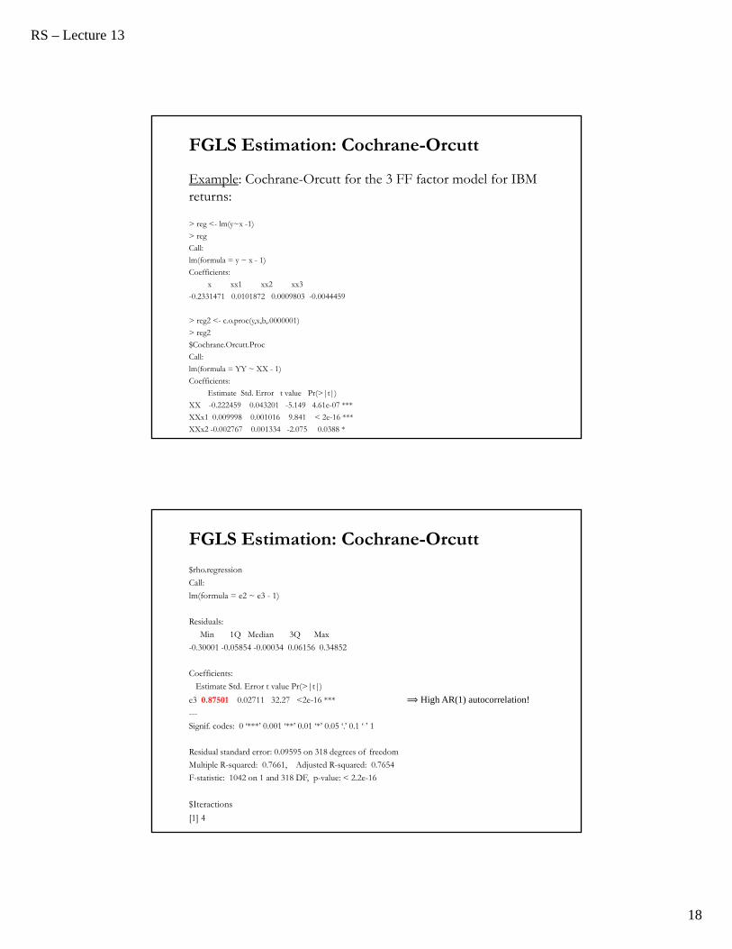
Example: Cochrane-Orcutt for the 3 FF factor model for IBM returns:
> reg <- lm(y~x -1)
> reg
Call:
lm(formula = y ~ x - 1)
Coefficients:
x xx1 xx2 xx3
-0.2331471 0.0101872 0.0009803 -0.0044459
> reg2 <- c.o.proc(y,x,b,.0000001)
> reg2
$Cochrane.Orcutt.Proc
Call:
lm(formula = YY ~ XX - 1)
Coefficients:
Estimate Std. Error t value Pr(>|t|)
XX -0.222459 0.043201 -5.149 4.61e-07 ***
XXx1 0.009998 0.001016 9.841 < 2e-16 ***
XXx2 -0.002767 0.001334 -2.075 0.0388 *
XX 3 0 003927 0 001565 2 510 0 0126 *
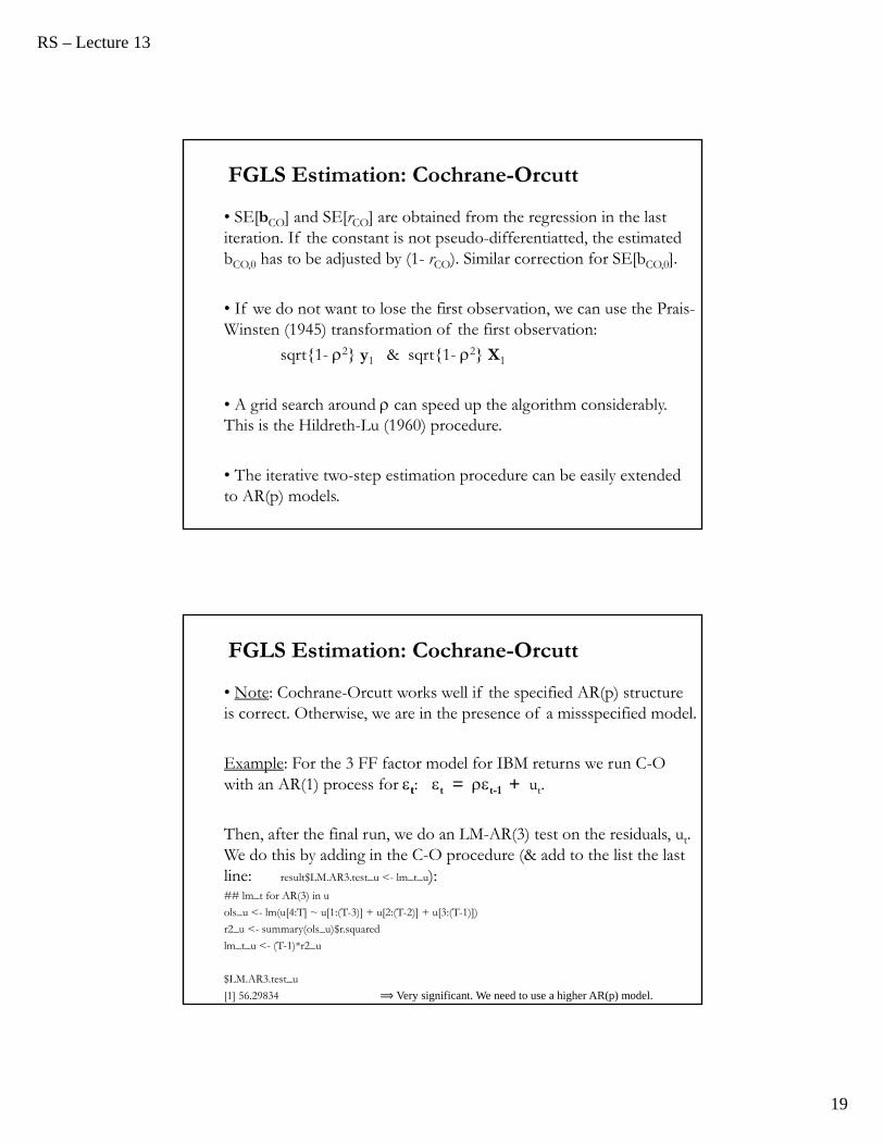
FGLS Estimation: Cochrane-Orcutt
$rho.regression
Call:
lm(formula = e2 ~ e3 - 1)
Residuals:
Min 1Q Median 3Q Max
-0.30001 -0.05854 -0.00034 0.06156 0.34852
Coefficients:
Estimate Std. Error t value Pr(>|t|)
e3 0.87501 0.02711 32.27 <2e-16 *** ⟹ High AR(1) autocorrelation!---
Signif. codes: 0 ‘***’ 0.001 ‘**’ 0.01 ‘*’ 0.05 ‘.’ 0.1 ‘ ’ 1
Residual standard error: 0.09595 on 318 degrees of freedom
Multiple R-squared: 0.7661, Adjusted R-squared: 0.7654
F-statistic: 1042 on 1 and 318 DF, p-value: < 2.2e-16
$Iteractions
[1] 4
FGLS Estimation: Cochrane-Orcutt
RS – Lecture 13
19
• SE[bCO] and SE[rCO] are obtained from the regression in the last iteration. If the constant is not pseudo-differentiatted, the estimated bCO,0 has to be adjusted by (1- rCO). Similar correction for SE[bCO,0].
• If we do not want to lose the first observation, we can use the Prais-Winsten (1945) transformation of the first observation:
sqrt1- 2 y1 & sqrt1- 2 X1
• A grid search around can speed up the algorithm considerably. This is the Hildreth-Lu (1960) procedure.
• The iterative two-step estimation procedure can be easily extended to AR(p) models.
FGLS Estimation: Cochrane-Orcutt
• Note: Cochrane-Orcutt works well if the specified AR(p) structure is correct. Otherwise, we are in the presence of a missspecified model.
Example: For the 3 FF factor model for IBM returns we run C-O with an AR(1) process for t: t = t-1 + ut.
Then, after the final run, we do an LM-AR(3) test on the residuals, ut. We do this by adding in the C-O procedure (& add to the list the last line: result$LM.AR3.test_u <- lm_t_u):## lm_t for AR(3) in u
ols_u <- lm(u[4:T] ~ u[1:(T-3)] + u[2:(T-2)] + u[3:(T-1)])
r2_u <- summary(ols_u)$r.squared
lm_t_u <- (T-1)*r2_u
$LM.AR3.test_u
[1] 56.29834 ⟹ Very significant. We need to use a higher AR(p) model.
FGLS Estimation: Cochrane-Orcutt
RS – Lecture 13
20
FGLS & MLE Estimation
• We need to estimate ⟹ We need a model for = (θ).
⟹ In the AR(1) model, we had = ().
- FGLS estimation is done using Cochrane-Orcutt or NLLS.
- MLE can also be done, say assuming a normal distribution for ut, to estimate and simultaneously. For the AR(1) problem, the MLE algorithm works like the Cochrane-Orcutt algorithm.
• For an AR(2) model, Beach-Mackinnon (1978) propose an MLE algorithm that is very fast to converge.
• For an AR(p) models, with p > 3, MLE becomes complicated. Two-step estimation is usually done.
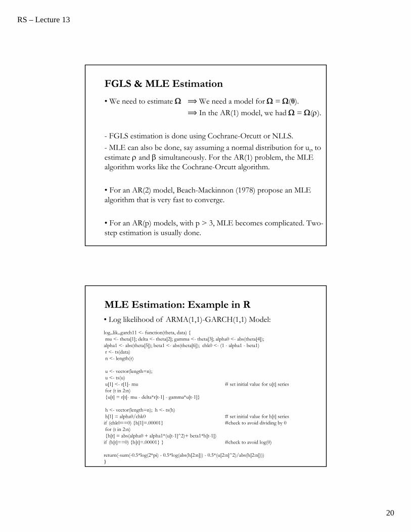
• Log likelihood of ARMA(1,1)-GARCH(1,1) Model:
log_lik_garch11 <- function(theta, data) mu <- theta[1]; delta <- theta[2]; gamma <- theta[3]; alpha0 <- abs(theta[4]); alpha1 <- abs(theta[5]); beta1 <- abs(theta[6]); chk0 <- (1 - alpha1 - beta1)r <- ts(data)n <- length(r)
u <- vector(length=n); u <- ts(u)u[1] <- r[1]- mu # set initial value for u[t] seriesfor (t in 2:n)u[t] = r[t]- mu - delta*r[t-1] - gamma*u[t-1]
h <- vector(length=n); h <- ts(h)h[1] = alpha0/chk0 # set initial value for h[t] seriesif (chk0==0) h[1]=.00001 #check to avoid dividing by 0for (t in 2:n)h[t] = abs(alpha0 + alpha1*(u[t-1]^2)+ beta1*h[t-1])if (h[t]==0) h[t]=.00001 #check to avoid log(0)
return(-sum(-0.5*log(2*pi) - 0.5*log(abs(h[2:n])) - 0.5*(u[2:n]^2)/abs(h[2:n])))
MLE Estimation: Example in R
RS – Lecture 13
21
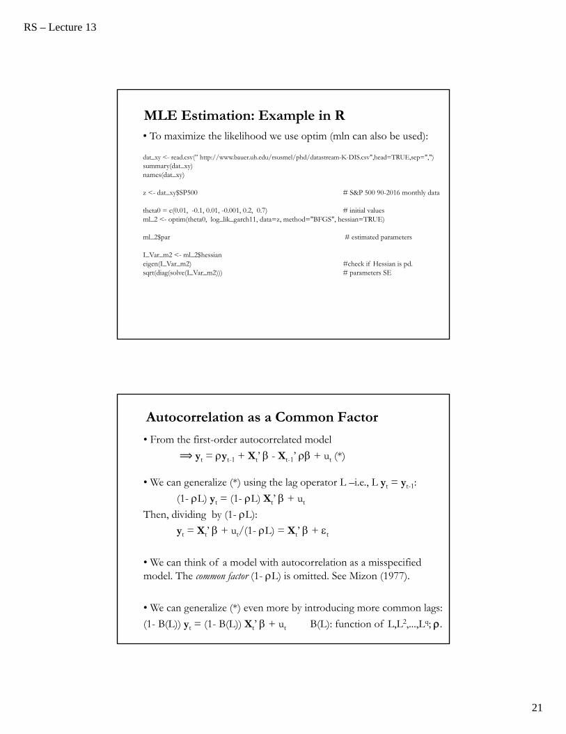
• To maximize the likelihood we use optim (mln can also be used):
dat_xy <- read.csv(” http://www.bauer.uh.edu/rsusmel/phd/datastream-K-DIS.csv",head=TRUE,sep=",")summary(dat_xy)names(dat_xy)
z <- dat_xy$SP500 # S&P 500 90-2016 monthly data
theta0 = c(0.01, -0.1, 0.01, -0.001, 0.2, 0.7) # initial valuesml_2 <- optim(theta0, log_lik_garch11, data=z, method="BFGS", hessian=TRUE)
ml_2$par # estimated parameters
I_Var_m2 <- ml_2$hessianeigen(I_Var_m2) #check if Hessian is pd.sqrt(diag(solve(I_Var_m2))) # parameters SE
MLE Estimation: Example in R
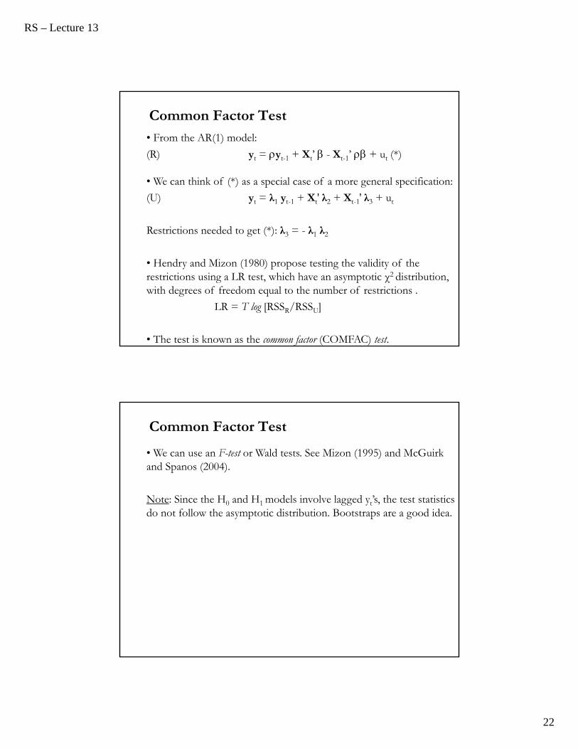
Autocorrelation as a Common Factor
• From the first-order autocorrelated model
⟹ yt = yt-1 + Xt’ - Xt-1’ + ut (*)
• We can generalize (*) using the lag operator L –i.e., L yt = yt-1:
(1- L) yt = (1- L) Xt’ + ut
Then, dividing by (1- L):
yt = Xt’ + ut/(1- L) = Xt’ + t
• We can think of a model with autocorrelation as a misspecified model. The common factor (1- L) is omitted. See Mizon (1977).
• We can generalize (*) even more by introducing more common lags:
(1- B(L)) yt = (1- B(L)) Xt’ + ut B(L): function of L,L2,...,Lq; .
RS – Lecture 13
22
Common Factor Test
• From the AR(1) model:
(R) yt = yt-1 + Xt’ - Xt-1’ + ut (*)
• We can think of (*) as a special case of a more general specification:
(U) yt = λ1 yt-1 + Xt′ λ2 + Xt-1′ λ3 + ut
Restrictions needed to get (*): λ3 = - λ1 λ2
• Hendry and Mizon (1980) propose testing the validity of the restrictions using a LR test, which have an asymptotic χ2 distribution, with degrees of freedom equal to the number of restrictions .
LR = T log [RSSR/RSSU]
• The test is known as the common factor (COMFAC) test.
• We can use an F-test or Wald tests. See Mizon (1995) and McGuirk and Spanos (2004).
Note: Since the H0 and H1 models involve lagged yt’s, the test statistics do not follow the asymptotic distribution. Bootstraps are a good idea.
Common Factor Test
RS – Lecture 13
23
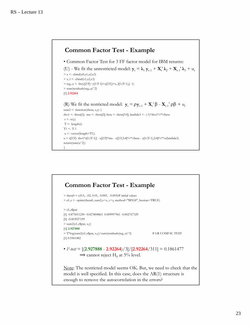
• Common Factor Test for 3 FF factor model for IBM returns:
(U) - We fit the unrestricted model: yt = λ1 yt-1 + Xt′ λ2 + Xt-1′ λ3 + ut> x <- cbind(x0,x1,x2,x3)
> x_l <- cbind(x1,x2,x3)
> reg_u <- lm(y[2:T]~y[1:T-1]+x[2:T,]+x_l[1:(T-1),] -1)
> sum(residuals(reg_u)^2)
[1] 2.92264
(R) We fit the restricted model: yt = yt-1 + Xt’ - Xt-1’ + utsum2 <- function(theta, x,y)
rho1 <- theta[1]; mu <- theta[2]; beta <- theta[3:5]; lambda3 <- (-1)*rho1%*%beta
r <- ts(y)
T <- length(r)
T1 <- T-1
u <- vector(length=T1);
u = r[2:T]- rho1*r[1:(T-1)] - x[2:T]*mu - x[2:T,2:4]%*%beta - x[1:(T-1),2:4]%*%t(lambda3)
return(sum(u^2))
Common Factor Test - Example
> theta0 = c(0.5, -.02, 0.01, -0.005, -0.003)# initial values
> cf_r <- optim(theta0, sum2,x=x, y=y, method="BFGS", hessian=TRUE)
> cf_r$par
[1] 0.875011230 -0.027804863 0.009997961 -0.002767329
[5] -0.003927199
> sum2(cf_r$par, x,y)
[1] 2.927888
> T*log(sum2(cf_r$par, x,y)/sum(residuals(reg_u)^2) # LR COMFAC TEST
[1] 0.5561482
• F-test = [(2.927888 - 2.92264)/3]/[2.92264/311] = 0.1861477 ⟹ cannot reject H0 at 5% level.
Note: The restricted model seems OK. But, we need to check that the model is well specified. In this case, does the AR(1) structure is enough to remove the autocorrelation in the errors?
Common Factor Test - Example
RS – Lecture 13
24
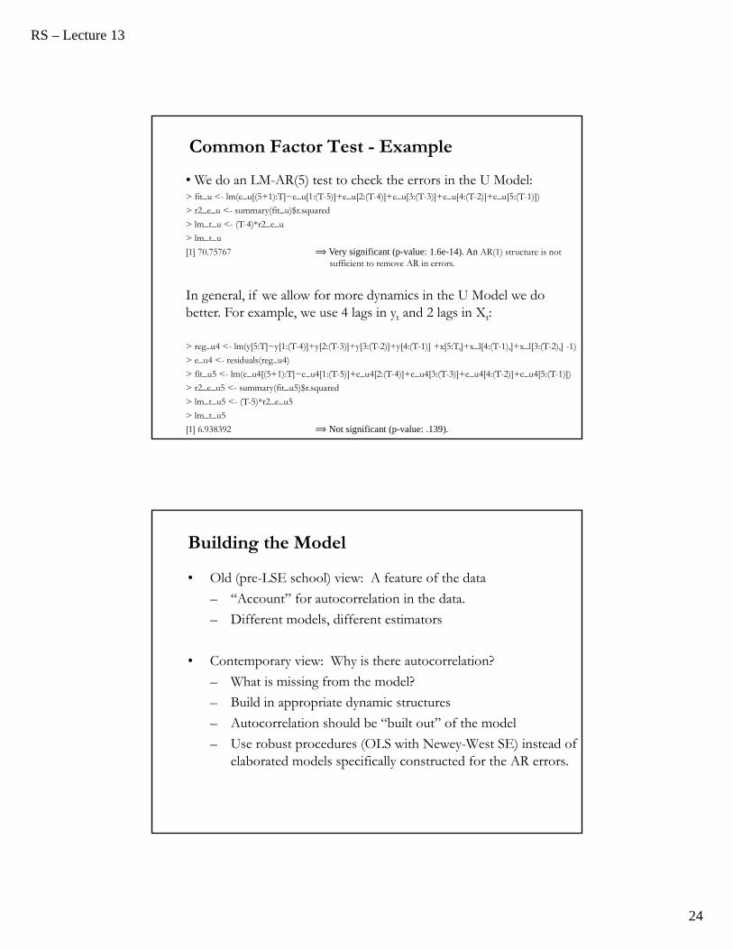
• We do an LM-AR(5) test to check the errors in the U Model:> fit_u <- lm(e_u[(5+1):T]~e_u[1:(T-5)]+e_u[2:(T-4)]+e_u[3:(T-3)]+e_u[4:(T-2)]+e_u[5:(T-1)])
> r2_e_u <- summary(fit_u)$r.squared
> lm_t_u <- (T-4)*r2_e_u
> lm_t_u
[1] 70.75767 ⟹ Very significant (p-value: 1.6e-14). An AR(1) structure is not sufficient to remove AR in errors.
In general, if we allow for more dynamics in the U Model we do better. For example, we use 4 lags in yt and 2 lags in Xt:
> reg_u4 <- lm(y[5:T]~y[1:(T-4)]+y[2:(T-3)]+y[3:(T-2)]+y[4:(T-1)] +x[5:T,]+x_l[4:(T-1),]+x_l[3:(T-2),] -1)
> e_u4 <- residuals(reg_u4)
> fit_u5 <- lm(e_u4[(5+1):T]~e_u4[1:(T-5)]+e_u4[2:(T-4)]+e_u4[3:(T-3)]+e_u4[4:(T-2)]+e_u4[5:(T-1)])
> r2_e_u5 <- summary(fit_u5)$r.squared
> lm_t_u5 <- (T-5)*r2_e_u5
> lm_t_u5
[1] 6.938392 ⟹ Not significant (p-value: .139).
Common Factor Test - Example
Building the Model
• Old (pre-LSE school) view: A feature of the data
– “Account” for autocorrelation in the data.
– Different models, different estimators
• Contemporary view: Why is there autocorrelation?
– What is missing from the model?
– Build in appropriate dynamic structures
– Autocorrelation should be “built out” of the model
– Use robust procedures (OLS with Newey-West SE) instead of elaborated models specifically constructed for the AR errors.


![α Physiologic correlation - medinfo2.psu.ac.thmedinfo2.psu.ac.th/pr/chest2012/chest2010/pdf/[12] Cases with physiologic correlation... · Morphology Physiology Physiology of lung](https://static.fdocument.org/doc/165x107/5d4b913888c99388658b7bf0/-physiologic-correlation-12-cases-with-physiologic-correlation-morphology.jpg)