Lecture 11: Parallel finite differences

Lecture 11: Parallel finite differences p. 1

Overview

1D heat equation ut = uxx + f(x, t) as example

Recapitulation of the finite difference method

Recapitulation of parallelization

Jacobi method for the steady-state case: uxx = g(x)

Relevant reading: Chapter 13 in Michael J. Quinn, ParallelProgramming in C with MPI and OpenMP

Lecture 11: Parallel finite differences p. 2

The heat equation

1D Example: temperature history of a thin metal rodu(x, t), for 0 < x < 1 and 0 < t T

Initial temperature distribution is known: u(x, 0) = I(x)

Temperature at both ends is zero: u(0, t) = u(1, t) = 0Heat conduction capability of the metal rod is knownHeat source is known

The 1D partial differential equation:

u

t=

2u

x2+ f(x, t)

u(x, t): the unknown function we want to find: known heat conductivity constantf(x, t): known heat source distribution

More compact notation: ut = uxx + f(x, t)

Lecture 11: Parallel finite differences p. 3

The finite difference method

A uniform spatial mesh: x0, x1, x2, . . . , xn, where xi = ix, x = 1n

Introduction of discrete time levels: t = t, t = Tm

Notation: ui = u(xi, t)

Derivatives are approximated by finite differences

u

t

u+1i ui

t

2u

x2

ui1 2ui + u

i+1

x2

Lecture 11: Parallel finite differences p. 4

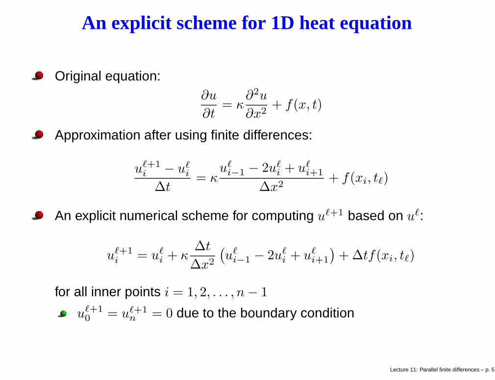
An explicit scheme for 1D heat equation

Original equation:u

t=

2u

x2+ f(x, t)

Approximation after using finite differences:

u+1i ui

t=

ui1 2ui + u

i+1

x2+ f(xi, t)

An explicit numerical scheme for computing u+1 based on u:

u+1i = ui +

t

x2(

ui1 2ui + u

i+1

)

+ tf(xi, t)

for all inner points i = 1, 2, . . . , n 1

u+10 = u+1n = 0 due to the boundary condition

Lecture 11: Parallel finite differences p. 5

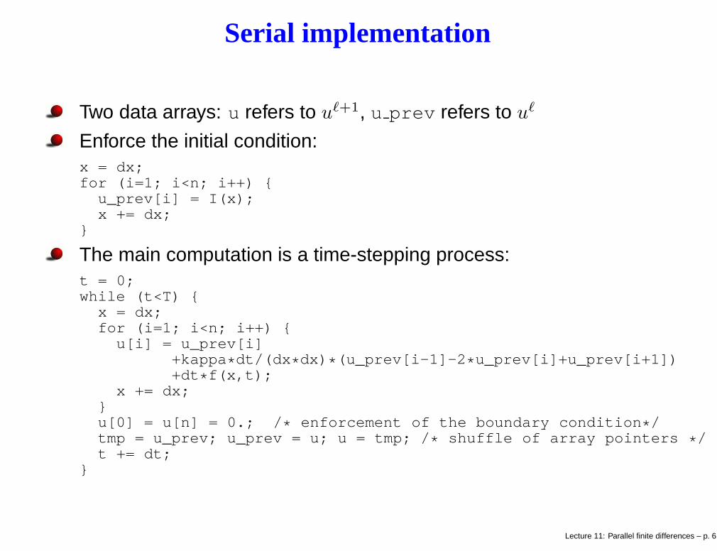
Serial implementation

Two data arrays: u refers to u+1, u prev refers to u

Enforce the initial condition:x = dx;for (i=1; i

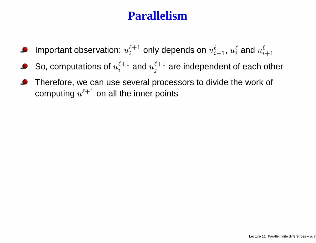
Parallelism

Important observation: u+1i only depends on ui1, u

i and u

i+1

So, computations of u+1i and u+1j are independent of each other

Therefore, we can use several processors to divide the work ofcomputing u+1 on all the inner points

Lecture 11: Parallel finite differences p. 7

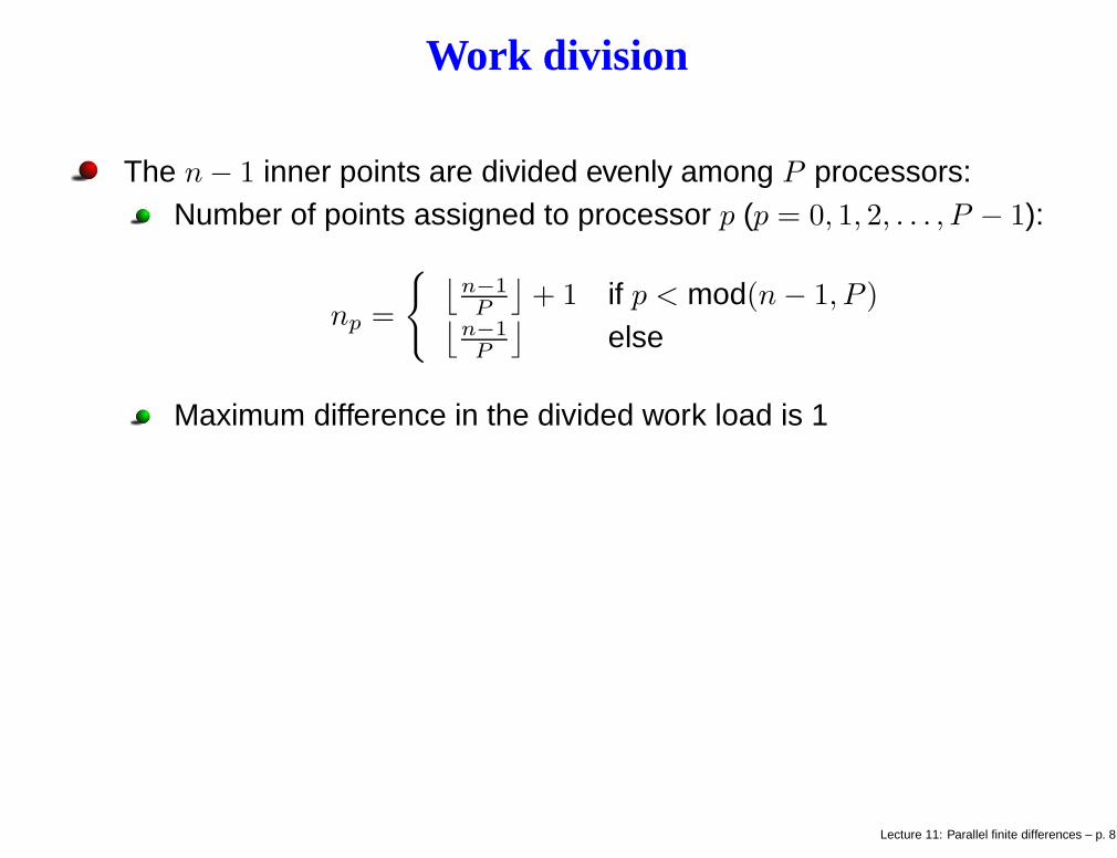
Work division

The n 1 inner points are divided evenly among P processors:Number of points assigned to processor p (p = 0, 1, 2, . . . , P 1):

np =

{

n1P

+ 1 if p < mod(n 1, P )

n1P

else

Maximum difference in the divided work load is 1

Lecture 11: Parallel finite differences p. 8

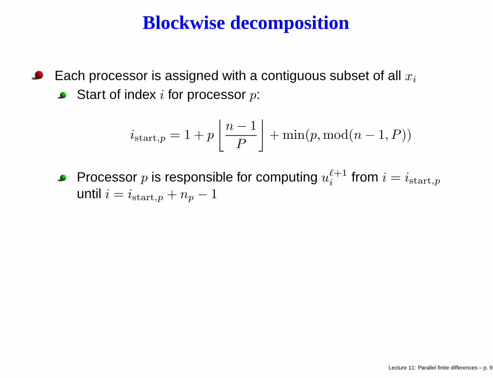
Blockwise decomposition

Each processor is assigned with a contiguous subset of all xiStart of index i for processor p:

istart,p = 1 + p

n 1

P

+ min(p, mod(n 1, P ))

Processor p is responsible for computing u+1i from i = istart,puntil i = istart,p + np 1

Lecture 11: Parallel finite differences p. 9

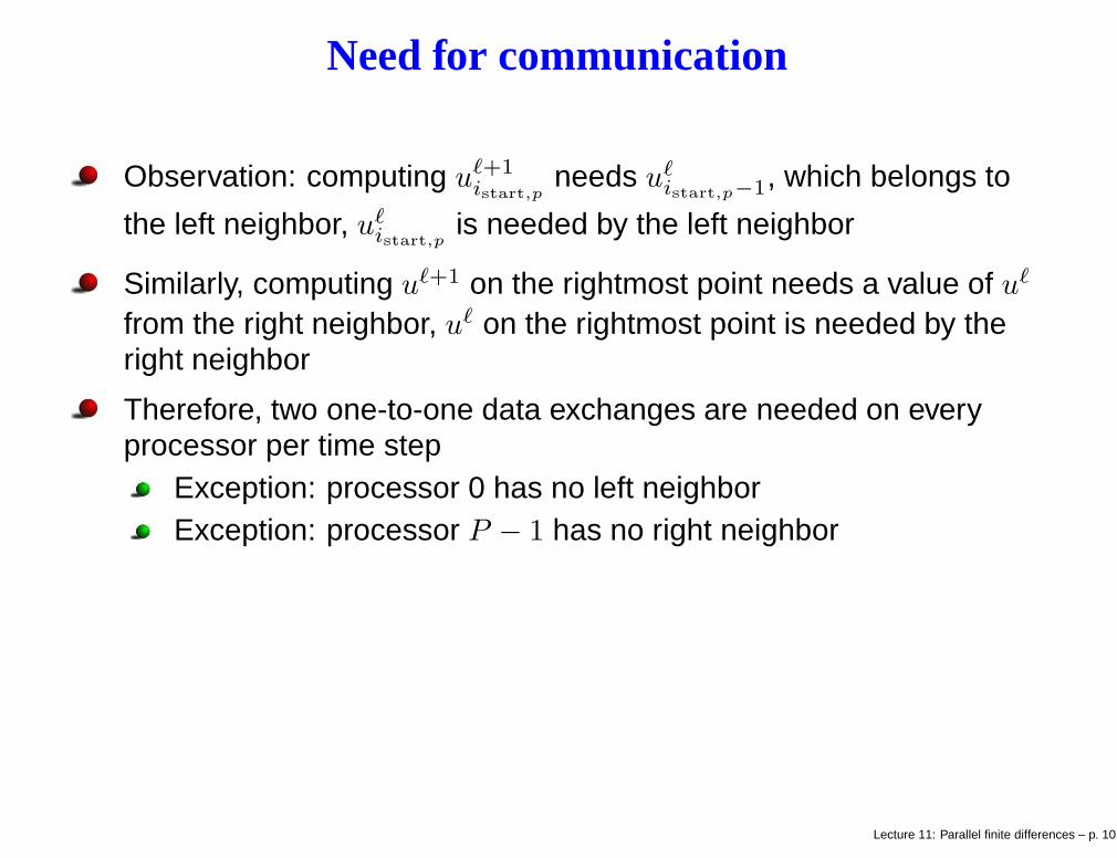
Need for communication

Observation: computing u+1istart,p needs uistart,p1

, which belongs to

the left neighbor, uistart,p is needed by the left neighbor

Similarly, computing u+1 on the rightmost point needs a value of u

from the right neighbor, u on the rightmost point is needed by theright neighbor

Therefore, two one-to-one data exchanges are needed on everyprocessor per time step

Exception: processor 0 has no left neighborException: processor P 1 has no right neighbor

Lecture 11: Parallel finite differences p. 10

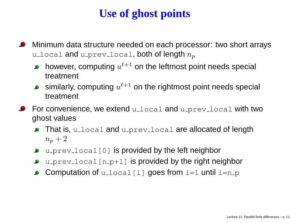
Use of ghost points

Minimum data structure needed on each processor: two short arraysu local and u prev local, both of length np

however, computing u+1 on the leftmost point needs specialtreatmentsimilarly, computing u+1 on the rightmost point needs specialtreatment

For convenience, we extend u local and u prev local with twoghost values

That is, u local and u prev local are allocated of lengthnp + 2

u prev local[0] is provided by the left neighboru prev local[n p+1] is provided by the right neighborComputation of u local[i] goes from i=1 until i=n p

Lecture 11: Parallel finite differences p. 11

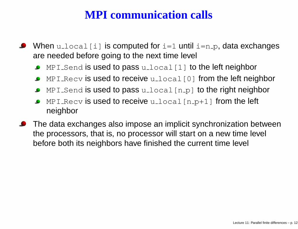
MPI communication calls

When u local[i] is computed for i=1 until i=n p, data exchangesare needed before going to the next time level

MPI Send is used to pass u local[1] to the left neighborMPI Recv is used to receive u local[0] from the left neighborMPI Send is used to pass u local[n p] to the right neighborMPI Recv is used to receive u local[n p+1] from the leftneighbor

The data exchanges also impose an implicit synchronization betweenthe processors, that is, no processor will start on a new time levelbefore both its neighbors have finished the current time level

Lecture 11: Parallel finite differences p. 12

Danger for deadlock

If two neighboring processors both start with MPI Recv and conitnuewith MPI Send, deadlock will arise because none can return from theMPI Recv call

Deadlock will probably not be a problem if both processors start withMPI Send and continue with MPI Recv

The safest approach is to use a rea-black coloring scheme:Processors with an odd rank are labeled as redProcessors with an even rank are labeled as blackOn red processor: first MPI Send then MPI RecvOn black processor: first MPI Recv then MPI Send

Lecture 11: Parallel finite differences p. 13

MPI_Sendrecv

The MPI Sendrecv command is designed to handle one-to-one dataexchangeMPI_Sendrecv(void *sendbuf, int sendcount, MPI_Datatype sendtype,

int dest, int sendtag,void *recvbuf, int recvcount, MPI_Datatype recvtype,int source, int recvtag,MPI_Comm comm, MPI_Status *status )

MPI PROC NULL can be used if the receiver or sender process doesnot exist

Note that processor 0 has no left neighborNote that processor P 1 has no right neighbor

Lecture 11: Parallel finite differences p. 14

Use of non-blocking MPI calls

Another way of avoiding deadlock is to use non-blocking MPI calls,for example, MPI Isend and MPI Irecv

However, the programmer typically has to make sure later that thecommunication tasks acutally complete by MPI Wait

A more important motivation for using non-blocking MPI calls is toexploit the possibility of communication and computation overlap hiding communication overhead

Lecture 11: Parallel finite differences p. 15

Stationary heat conduction

If the heat equation ut = uxx + f(x, t) reaches a steady state, thenut = 0 and f(x, t) = f(x)

The resulting 1D equation becomes

d2u

dx2= g(x)

where g(x) = f(x)/

Lecture 11: Parallel finite differences p. 16

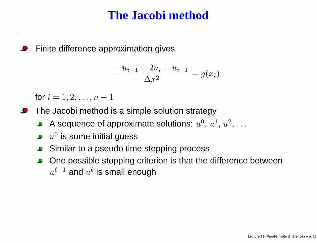
The Jacobi method

Finite difference approximation gives

ui1 + 2ui ui+1x2

= g(xi)

for i = 1, 2, . . . , n 1

The Jacobi method is a simple solution strategy

A sequence of approximate solutions: u0, u1, u2, . . .

u0 is some initial guessSimilar to a pseudo time stepping processOne possible stopping criterion is that the difference betweenu+1 and u is small enough

Lecture 11: Parallel finite differences p. 17

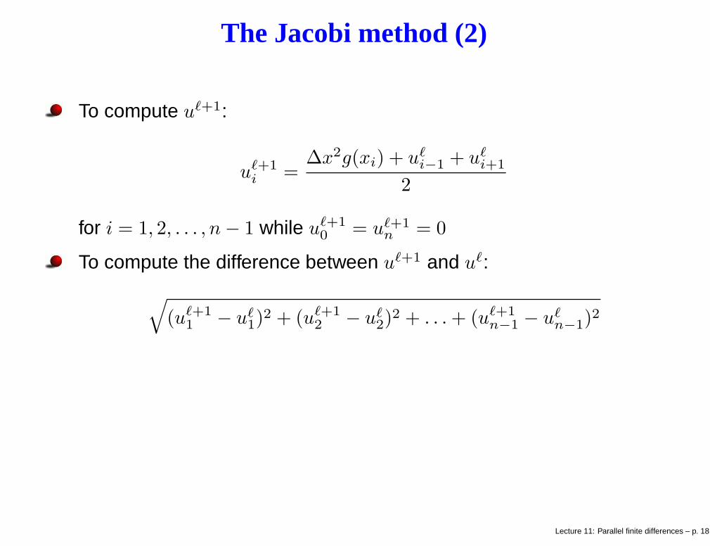
The Jacobi method (2)

To compute u+1:

u+1i =x2g(xi) + u

i1 + u

i+1

2

for i = 1, 2, . . . , n 1 while u+10 = u+1n = 0

To compute the difference between u+1 and u:

(u+11 u1)

2 + (u+12 u2)

2 + . . . + (u+1n1 un1)

2

Lecture 11: Parallel finite differences p. 18

Observations

The Jacobi method has the same parallelism as the explicit schemefor the time-dependent heat equation

Data partitioning is the same as before

In an MPI implementation, two arrays u local and u prev localare needed on each processor

Computing the difference between u+1 and u is also parallelizableFirst, every processor computes

diffp = (u+1p,1 up,1)

2 + (u+1p,2 up,2)

2 + . . . + (u+1p,np up,np

)2

Then all the diffp values are added up by a reduction operation,using MPI AllreduceThe summed value thereafter is applied with a square rootoperation

Lecture 11: Parallel finite differences p. 19

Comments

Parallelization of the Jacobi method requires both one-to-onecommunication and collective communication

There are more advanced solution strategies (than Jacobi) for solvingthe steady-state heat equation

Parallelization is not necessarily more difficult

2D/3D heat equations (both time-dependent and steady-state) canbe handled by the same principles

Lecture 11: Parallel finite differences p. 20

Exercise

Make an MPI implementation of the Jacobi method for solving a 2Dsteady-state heat equation

Lecture 11: Parallel finite differences p. 21

OverviewThe heat equationThe finite difference methodAn explicit scheme for 1D heat equationSerial implementationParallelismWork divisionBlockwise decompositionNeed for communicationUse of ghost pointsMPI communication callsDanger for deadlockMPI_SendrecvUse of non-blocking MPI callsStationary heat conductionThe Jacobi methodThe Jacobi method (2)ObservationsCommentsExercise