Lecture 10: Logistical Regression II— Multinomial Data
73
Lecture 10: Logistical Regression II— Multinomial Data Prof. Sharyn O’Halloran Sustainable Development U9611 Econometrics II
-
Upload
nguyenxuyen -
Category
Documents
-
view
224 -
download
1
Transcript of Lecture 10: Logistical Regression II— Multinomial Data

Lecture 10: Logistical Regression II—Multinomial Data
Prof. Sharyn O’Halloran Sustainable Development U9611Econometrics II
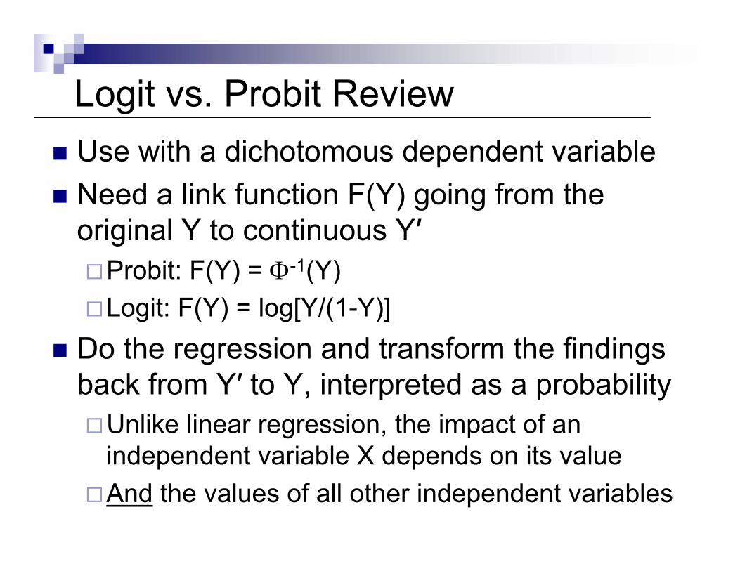
Logit vs. Probit ReviewUse with a dichotomous dependent variableNeed a link function F(Y) going from the original Y to continuous Y′
Probit: F(Y) = Φ-1(Y)Logit: F(Y) = log[Y/(1-Y)]
Do the regression and transform the findings back from Y′ to Y, interpreted as a probability
Unlike linear regression, the impact of an independent variable X depends on its valueAnd the values of all other independent variables
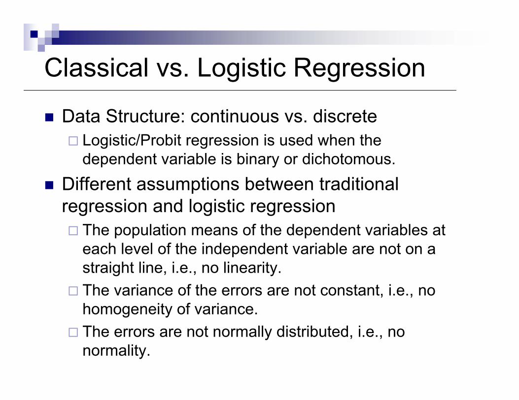
Classical vs. Logistic Regression
Data Structure: continuous vs. discrete Logistic/Probit regression is used when the dependent variable is binary or dichotomous.
Different assumptions between traditional regression and logistic regression
The population means of the dependent variables at each level of the independent variable are not on a straight line, i.e., no linearity. The variance of the errors are not constant, i.e., no homogeneity of variance. The errors are not normally distributed, i.e., no normality.
Logistic Regression Assumptions 1. The model is correctly specified, i.e.,
The true conditional probabilities are a logistic function of the independent variables;No important variables are omitted;No extraneous variables are included; andThe independent variables are measured without error.
2. The cases are independent. 3. The independent variables are not linear
combinations of each other. Perfect multicollinearity makes estimation impossible, While strong multicollinearity makes estimates imprecise.
About Logistic Regression It uses a maximum likelihood estimation rather than the least squares estimation used in traditional multiple regression. The general form of the distribution is assumed. Starting values of the estimated parameters are used and the likelihood that the sample came from a population with those parameters is computed. The values of the estimated parameters are adjusted iteratively until the maximum likelihood value for the estimated parameters is obtained.
That is, maximum likelihood approaches try to find estimates of parameters that make the data actually observed "most likely."
Interpreting Logistic CoefficientsLogistic slope coefficients can be interpreted as the effect of a unit of change in the X variable on the predicted logits with the other variables in the model held constant.
That is, how a one unit change in X effects the log of the odds when the other variables in the model held constant.
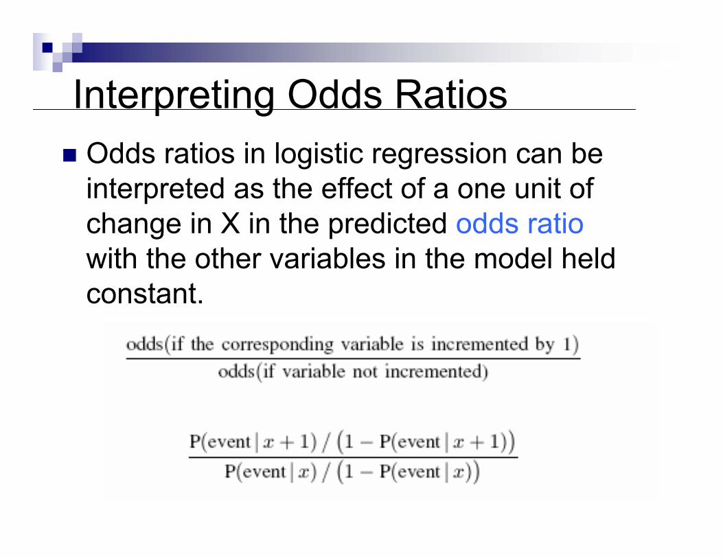
Interpreting Odds Ratios Odds ratios in logistic regression can be interpreted as the effect of a one unit of change in X in the predicted odds ratiowith the other variables in the model held constant.
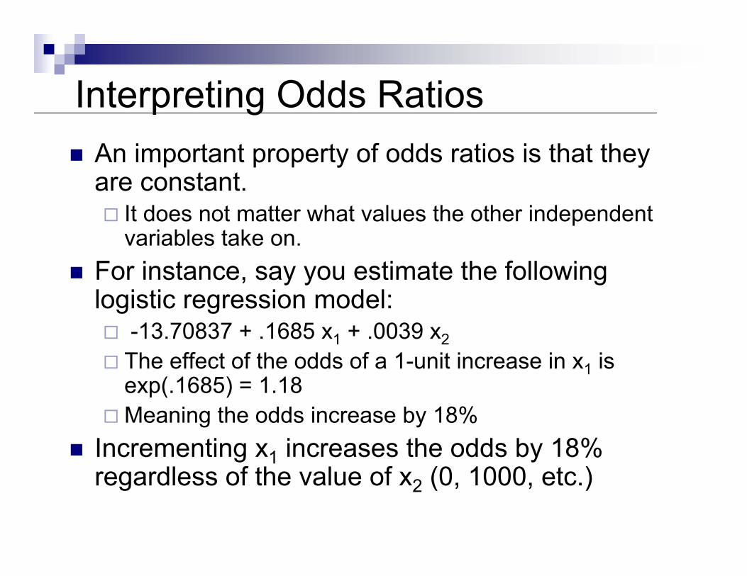
Interpreting Odds Ratios An important property of odds ratios is that they are constant.
It does not matter what values the other independent variables take on.
For instance, say you estimate the following logistic regression model:
-13.70837 + .1685 x1 + .0039 x2The effect of the odds of a 1-unit increase in x1 is exp(.1685) = 1.18Meaning the odds increase by 18%
Incrementing x1 increases the odds by 18% regardless of the value of x2 (0, 1000, etc.)
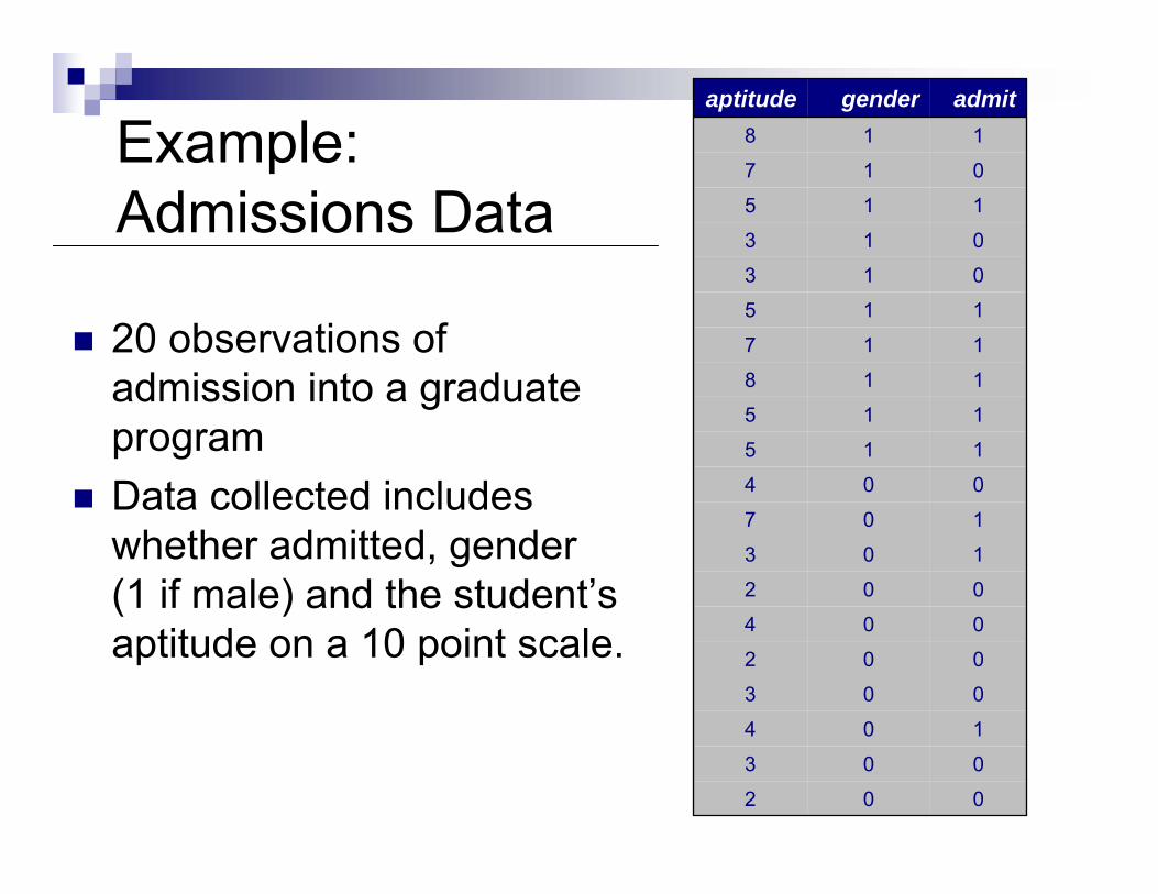
Example: Admissions Data
20 observations of admission into a graduate programData collected includes whether admitted, gender (1 if male) and the student’s aptitude on a 10 point scale.
002
003
104
003
002
004
002
103
107
004
115
115
118
117
115
013
013
115
017
118
admitgender aptitude
Admissions Example – Calculating the Odds Ratio
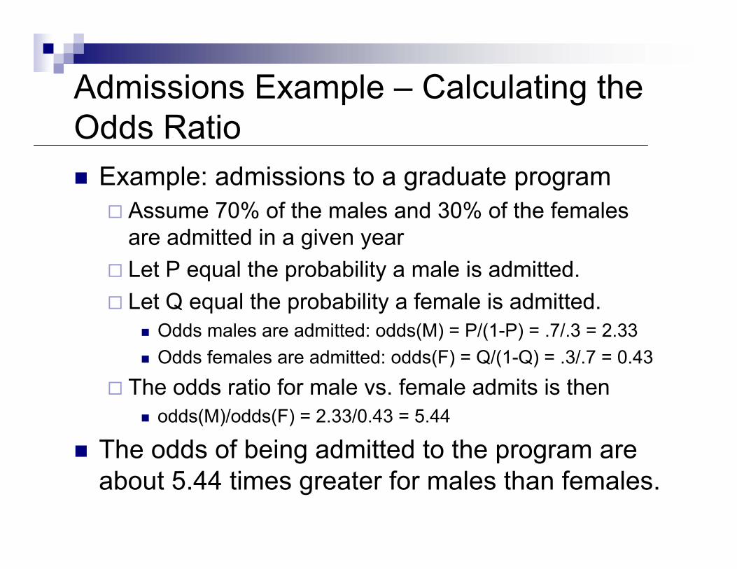
Example: admissions to a graduate programAssume 70% of the males and 30% of the females are admitted in a given yearLet P equal the probability a male is admitted. Let Q equal the probability a female is admitted.
Odds males are admitted: odds(M) = P/(1-P) = .7/.3 = 2.33 Odds females are admitted: odds(F) = Q/(1-Q) = .3/.7 = 0.43
The odds ratio for male vs. female admits is thenodds(M)/odds(F) = 2.33/0.43 = 5.44
The odds of being admitted to the program are about 5.44 times greater for males than females.
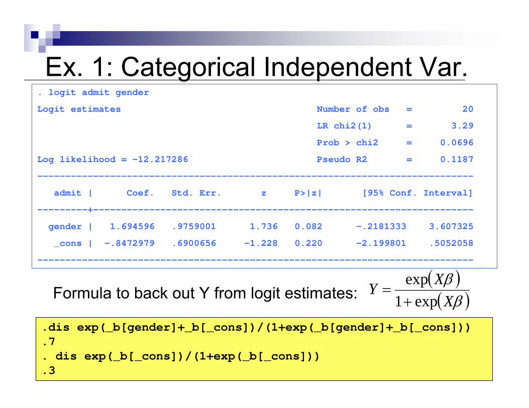
Ex. 1: Categorical Independent Var.. logit admit gender
Logit estimates Number of obs = 20
LR chi2(1) = 3.29
Prob > chi2 = 0.0696
Log likelihood = -12.217286 Pseudo R2 = 0.1187
------------------------------------------------------------------------------
admit | Coef. Std. Err. z P>|z| [95% Conf. Interval]
---------+--------------------------------------------------------------------
gender | 1.694596 .9759001 1.736 0.082 -.2181333 3.607325
_cons | -.8472979 .6900656 -1.228 0.220 -2.199801 .5052058
------------------------------------------------------------------------------
.dis exp(_b[gender]+_b[_cons])/(1+exp(_b[gender]+_b[_cons]))
.7
. dis exp(_b[_cons])/(1+exp(_b[_cons]))
.3
Formula to back out Y from logit estimates: ( )( )ββX
XYexp1
exp+
=
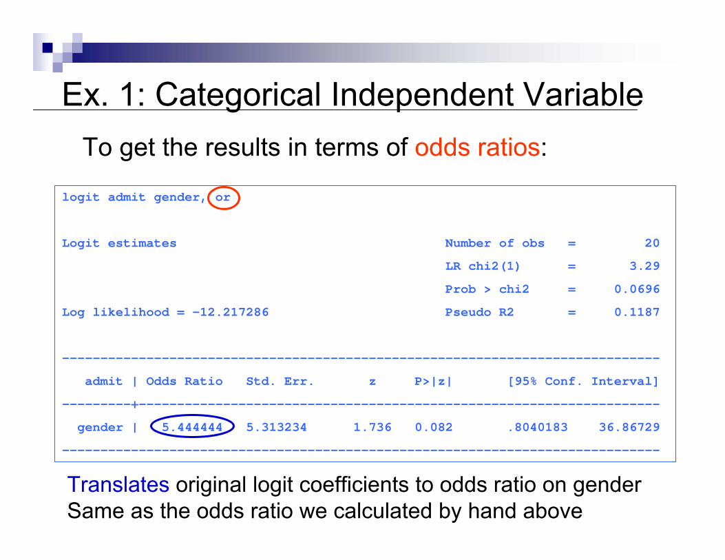
Ex. 1: Categorical Independent Variable
logit admit gender, or
Logit estimates Number of obs = 20
LR chi2(1) = 3.29
Prob > chi2 = 0.0696
Log likelihood = -12.217286 Pseudo R2 = 0.1187
------------------------------------------------------------------------------
admit | Odds Ratio Std. Err. z P>|z| [95% Conf. Interval]
---------+--------------------------------------------------------------------
gender | 5.444444 5.313234 1.736 0.082 .8040183 36.86729
------------------------------------------------------------------------------
To get the results in terms of odds ratios:
Translates original logit coefficients to odds ratio on genderSame as the odds ratio we calculated by hand above
Ex. 1: Categorical Independent Variable
logit admit gender, or
Logit estimates Number of obs = 20
LR chi2(1) = 3.29
Prob > chi2 = 0.0696
Log likelihood = -12.217286 Pseudo R2 = 0.1187
------------------------------------------------------------------------------
admit | Odds Ratio Std. Err. z P>|z| [95% Conf. Interval]
---------+--------------------------------------------------------------------
gender | 5.444444 5.313234 1.736 0.082 .8040183 36.86729
------------------------------------------------------------------------------
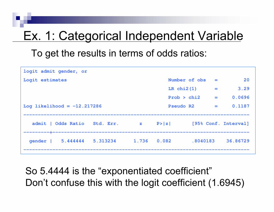
To get the results in terms of odds ratios:
So 5.4444 is the “exponentiated coefficient”Don’t confuse this with the logit coefficient (1.6945)
Ex. 1: Categorical Independent Variable
logit admit gender, or
Logit estimates Number of obs = 20
LR chi2(1) = 3.29
Prob > chi2 = 0.0696
Log likelihood = -12.217286 Pseudo R2 = 0.1187
------------------------------------------------------------------------------
admit | Odds Ratio Std. Err. z P>|z| [95% Conf. Interval]
---------+--------------------------------------------------------------------
gender | 5.444444 5.313234 1.736 0.082 .8040183 36.86729
------------------------------------------------------------------------------
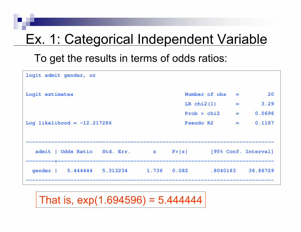
To get the results in terms of odds ratios:
That is, exp(1.694596) = 5.444444
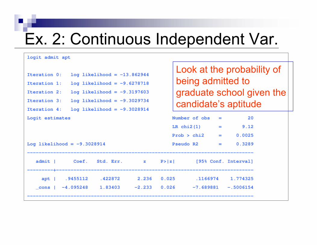
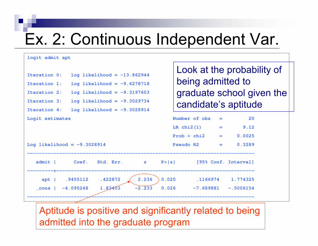
Ex. 2: Continuous Independent Var.logit admit apt
Iteration 0: log likelihood = -13.862944
Iteration 1: log likelihood = -9.6278718
Iteration 2: log likelihood = -9.3197603
Iteration 3: log likelihood = -9.3029734
Iteration 4: log likelihood = -9.3028914
Logit estimates Number of obs = 20
LR chi2(1) = 9.12
Prob > chi2 = 0.0025
Log likelihood = -9.3028914 Pseudo R2 = 0.3289
------------------------------------------------------------------------------
admit | Coef. Std. Err. z P>|z| [95% Conf. Interval]
---------+--------------------------------------------------------------------
apt | .9455112 .422872 2.236 0.025 .1166974 1.774325
_cons | -4.095248 1.83403 -2.233 0.026 -7.689881 -.5006154
------------------------------------------------------------------------------
Look at the probability of being admitted to graduate school given the candidate’s aptitude
Aptitude is positive and significantly related to being admitted into the graduate program
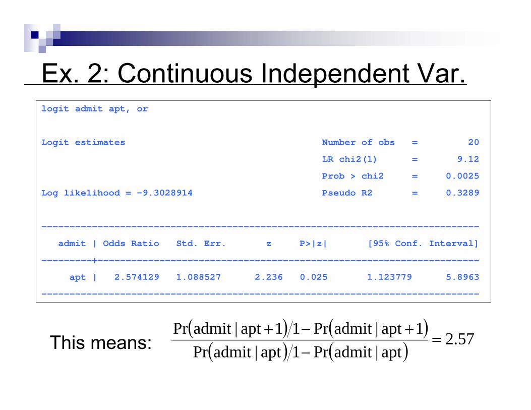
Ex. 2: Continuous Independent Var.logit admit apt, or
Logit estimates Number of obs = 20
LR chi2(1) = 9.12
Prob > chi2 = 0.0025
Log likelihood = -9.3028914 Pseudo R2 = 0.3289
------------------------------------------------------------------------------
admit | Odds Ratio Std. Err. z P>|z| [95% Conf. Interval]
---------+--------------------------------------------------------------------
apt | 2.574129 1.088527 2.236 0.025 1.123779 5.8963
------------------------------------------------------------------------------
This means:( ) ( )
( ) ( ) 57.2apt|admitPr1apt|admitPr
1apt|admitPr11apt|admitPr=
−+−+
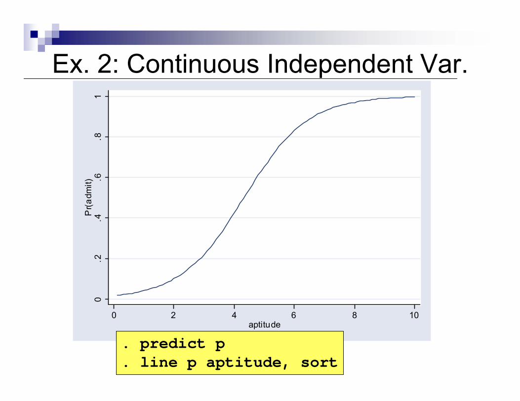
Ex. 2: Continuous Independent Var.0
.2.4
.6.8
1P
r(adm
it)
0 2 4 6 8 10aptitude
. predict p
. line p aptitude, sort
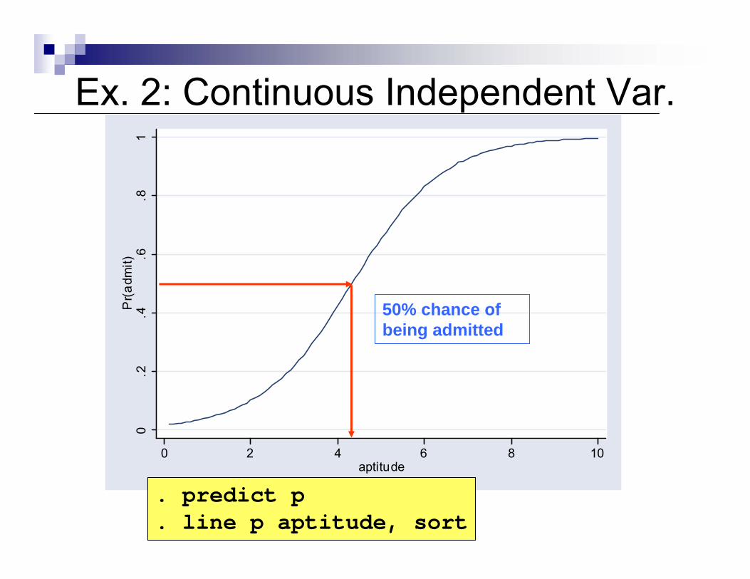
Ex. 2: Continuous Independent Var.0
.2.4
.6.8
1P
r(adm
it)
0 2 4 6 8 10aptitude
. predict p
. line p aptitude, sort
50% chance of being admitted
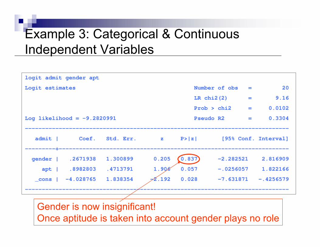
Example 3: Categorical & Continuous Independent Variables
logit admit gender apt
Logit estimates Number of obs = 20
LR chi2(2) = 9.16
Prob > chi2 = 0.0102
Log likelihood = -9.2820991 Pseudo R2 = 0.3304
------------------------------------------------------------------------------
admit | Coef. Std. Err. z P>|z| [95% Conf. Interval]
---------+--------------------------------------------------------------------
gender | .2671938 1.300899 0.205 0.837 -2.282521 2.816909
apt | .8982803 .4713791 1.906 0.057 -.0256057 1.822166
_cons | -4.028765 1.838354 -2.192 0.028 -7.631871 -.4256579
------------------------------------------------------------------------------
Gender is now insignificant!Once aptitude is taken into account gender plays no role
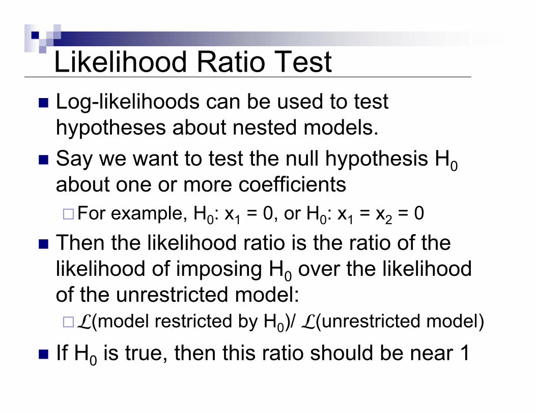
Likelihood Ratio TestLog-likelihoods can be used to test hypotheses about nested models.Say we want to test the null hypothesis H0about one or more coefficients
For example, H0: x1 = 0, or H0: x1 = x2 = 0Then the likelihood ratio is the ratio of the likelihood of imposing H0 over the likelihood of the unrestricted model:L(model restricted by H0)/ L(unrestricted model)
If H0 is true, then this ratio should be near 1
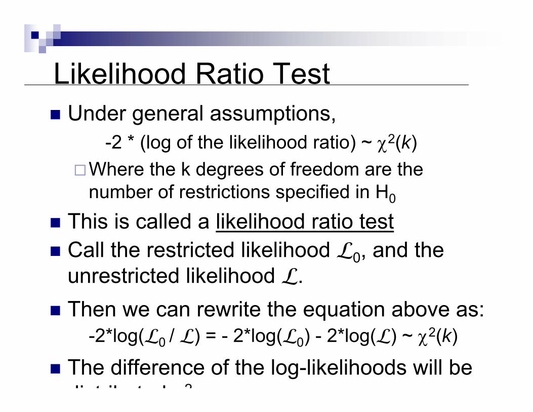
Likelihood Ratio TestUnder general assumptions,
-2 * (log of the likelihood ratio) ~ χ2(k)Where the k degrees of freedom are the number of restrictions specified in H0
This is called a likelihood ratio testCall the restricted likelihood L0, and the unrestricted likelihood L.Then we can rewrite the equation above as:
-2*log(L0 / L) = - 2*log(L0) - 2*log(L) ~ χ2(k)
The difference of the log-likelihoods will be di t ib t d 2
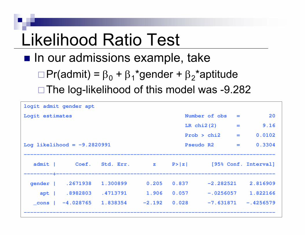
Likelihood Ratio TestIn our admissions example, take
Pr(admit) = β0 + β1*gender + β2*aptitudeThe log-likelihood of this model was -9.282
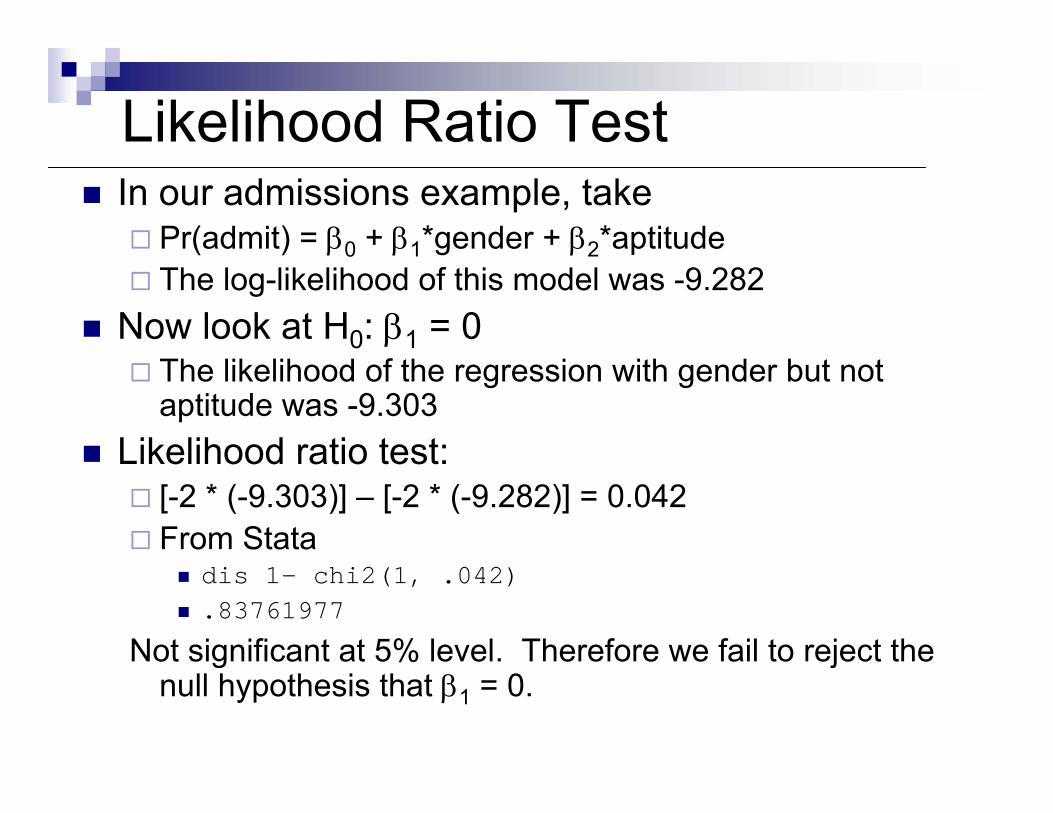
Likelihood Ratio TestIn our admissions example, take
Pr(admit) = β0 + β1*gender + β2*aptitudeThe log-likelihood of this model was -9.282
logit admit gender apt
Logit estimates Number of obs = 20
LR chi2(2) = 9.16
Prob > chi2 = 0.0102
Log likelihood = -9.2820991 Pseudo R2 = 0.3304
------------------------------------------------------------------------------
admit | Coef. Std. Err. z P>|z| [95% Conf. Interval]
---------+--------------------------------------------------------------------
gender | .2671938 1.300899 0.205 0.837 -2.282521 2.816909
apt | .8982803 .4713791 1.906 0.057 -.0256057 1.822166
_cons | -4.028765 1.838354 -2.192 0.028 -7.631871 -.4256579
------------------------------------------------------------------------------
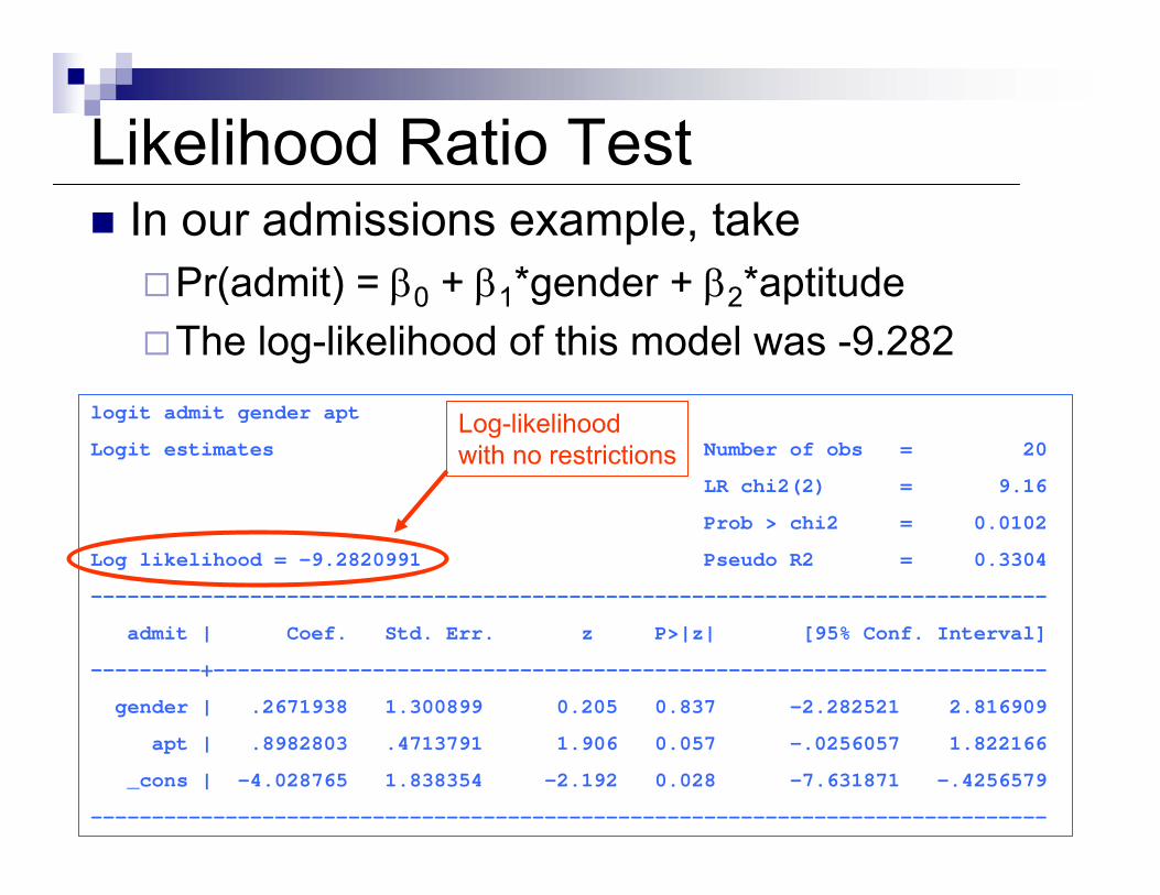
Log-likelihoodwith no restrictions
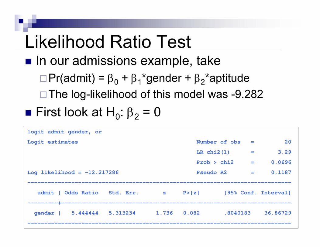
Likelihood Ratio TestIn our admissions example, take
Pr(admit) = β0 + β1*gender + β2*aptitudeThe log-likelihood of this model was -9.282
First look at H0: β2 = 0logit admit gender, or
Logit estimates Number of obs = 20
LR chi2(1) = 3.29
Prob > chi2 = 0.0696
Log likelihood = -12.217286 Pseudo R2 = 0.1187
------------------------------------------------------------------------------
admit | Odds Ratio Std. Err. z P>|z| [95% Conf. Interval]
---------+--------------------------------------------------------------------
gender | 5.444444 5.313234 1.736 0.082 .8040183 36.86729
------------------------------------------------------------------------------
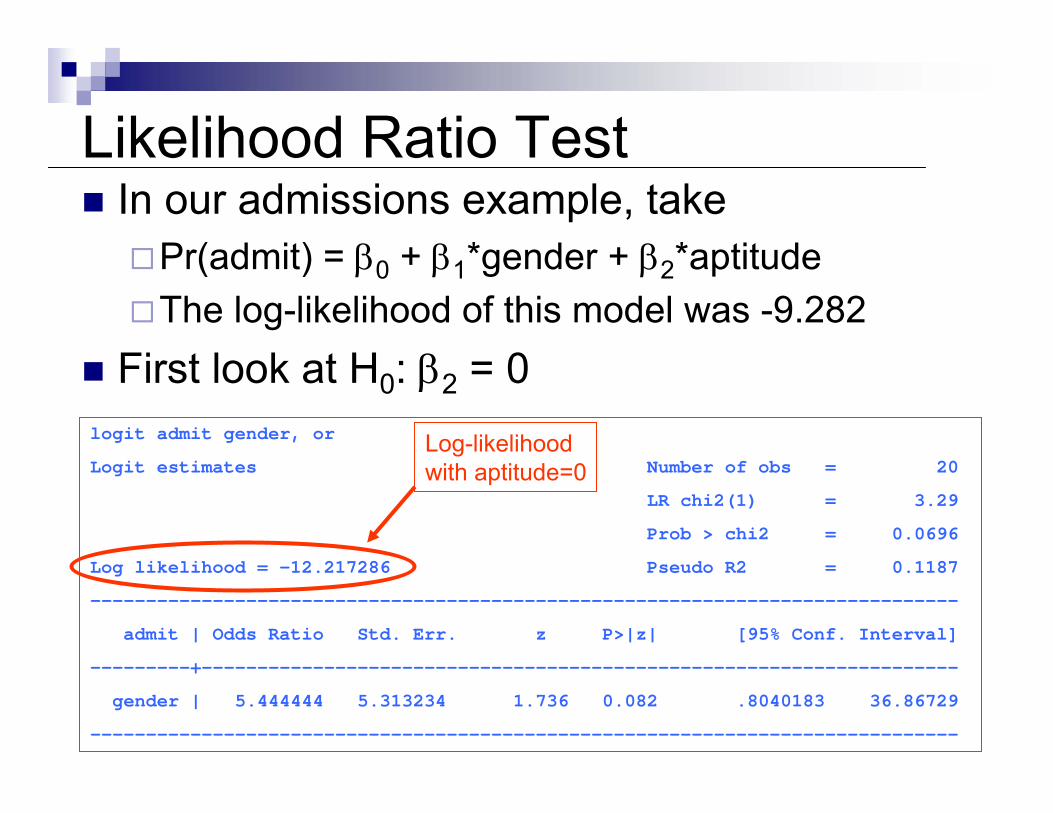
Log-likelihoodwith aptitude=0
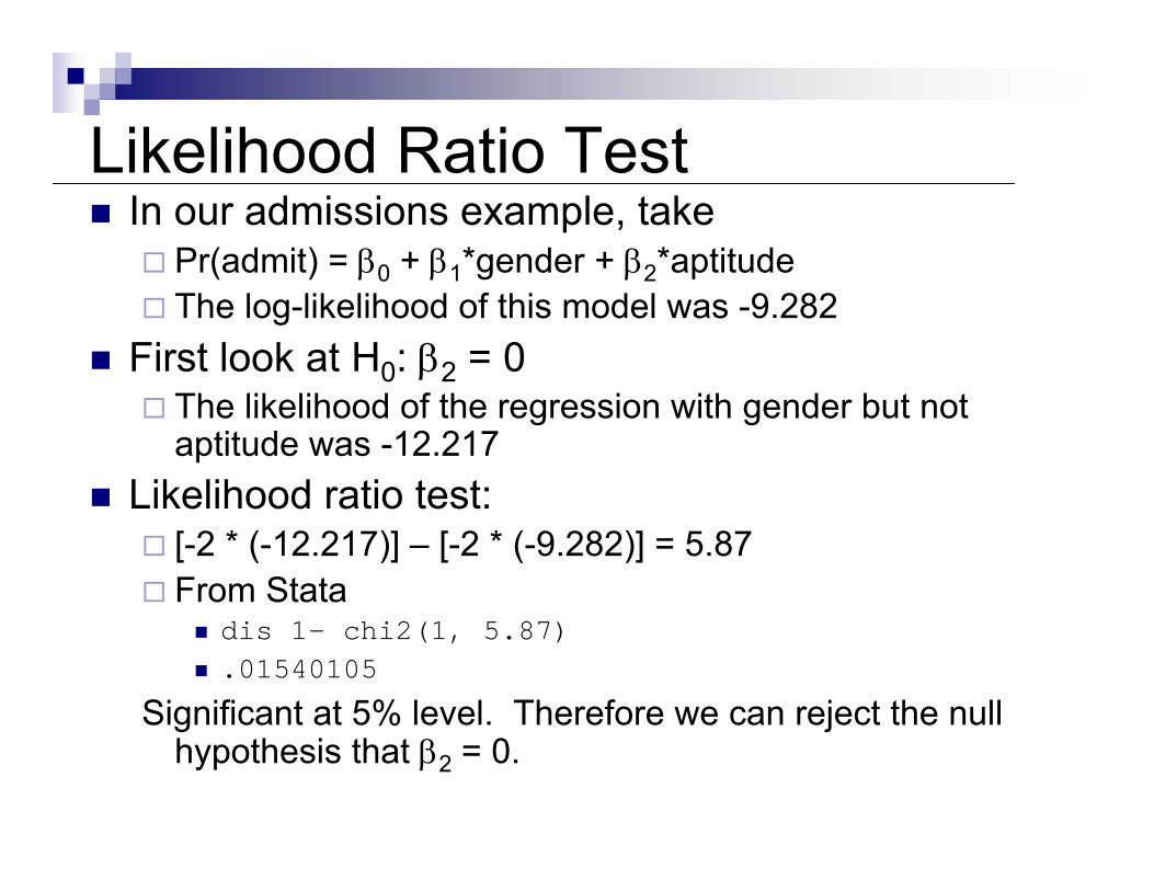
Likelihood Ratio TestIn our admissions example, take
Pr(admit) = β0 + β1*gender + β2*aptitudeThe log-likelihood of this model was -9.282
First look at H0: β2 = 0The likelihood of the regression with gender but not aptitude was -12.217
Likelihood ratio test:[-2 * (-12.217)] – [-2 * (-9.282)] = 5.87From Stata
dis 1- chi2(1, 5.87).01540105
Significant at 5% level. Therefore we can reject the null hypothesis that β2 = 0.
Likelihood Ratio TestIn our admissions example, take
Pr(admit) = β0 + β1*gender + β2*aptitudeThe log-likelihood of this model was -9.282
Now look at H0: β1 = 0
logit admit apt, or
Logit estimates Number of obs = 20
LR chi2(1) = 9.12
Prob > chi2 = 0.0025
Log likelihood = -9.3028914 Pseudo R2 = 0.3289
------------------------------------------------------------------------------
admit | Odds Ratio Std. Err. z P>|z| [95% Conf. Interval]
---------+--------------------------------------------------------------------
apt | 2.574129 1.088527 2.236 0.025 1.123779 5.8963
------------------------------------------------------------------------------
Likelihood Ratio TestIn our admissions example, take
Pr(admit) = β0 + β1*gender + β2*aptitudeThe log-likelihood of this model was -9.282
Now look at H0: β1 = 0
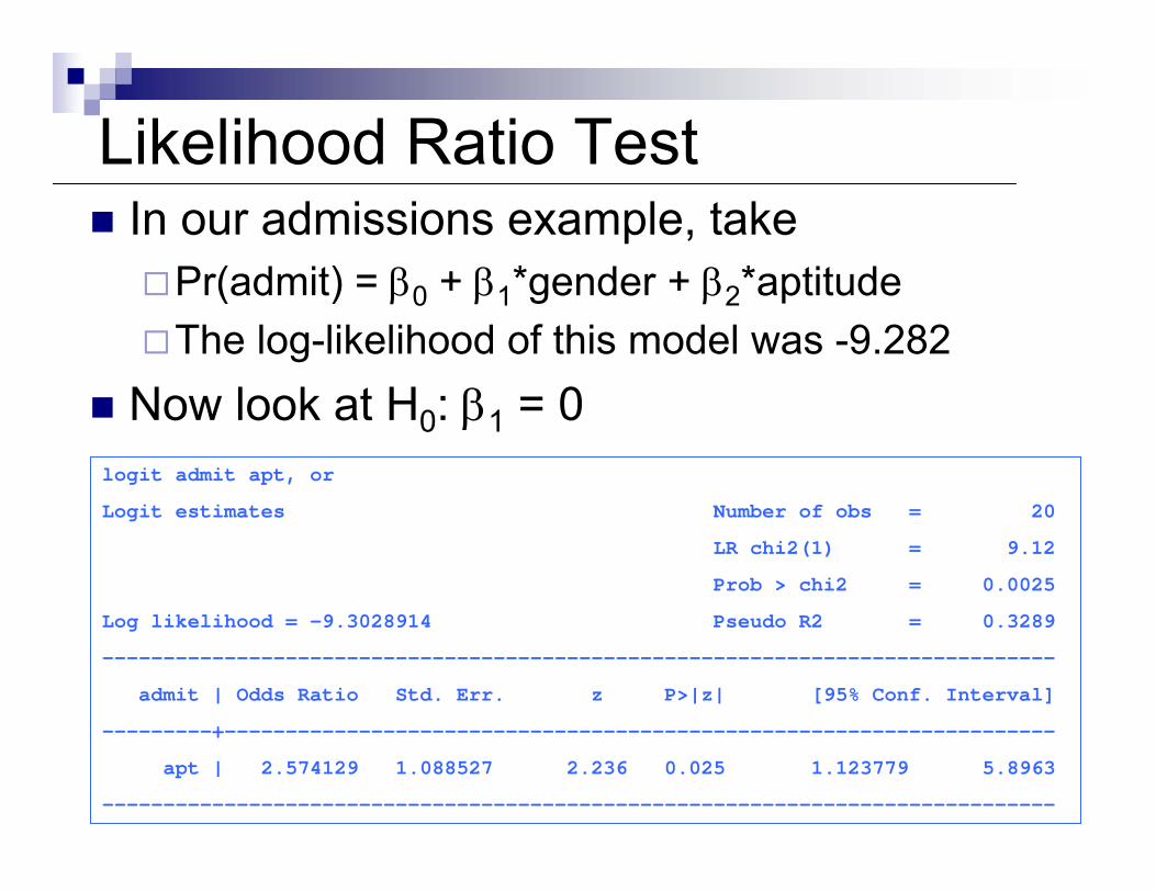
Likelihood Ratio TestIn our admissions example, take
Pr(admit) = β0 + β1*gender + β2*aptitudeThe log-likelihood of this model was -9.282
Now look at H0: β1 = 0Log-likelihoodwith gender=0
logit admit apt, or
Logit estimates Number of obs = 20
LR chi2(1) = 9.12
Prob > chi2 = 0.0025
Log likelihood = -9.3028914 Pseudo R2 = 0.3289
------------------------------------------------------------------------------
admit | Odds Ratio Std. Err. z P>|z| [95% Conf. Interval]
---------+--------------------------------------------------------------------
apt | 2.574129 1.088527 2.236 0.025 1.123779 5.8963
------------------------------------------------------------------------------
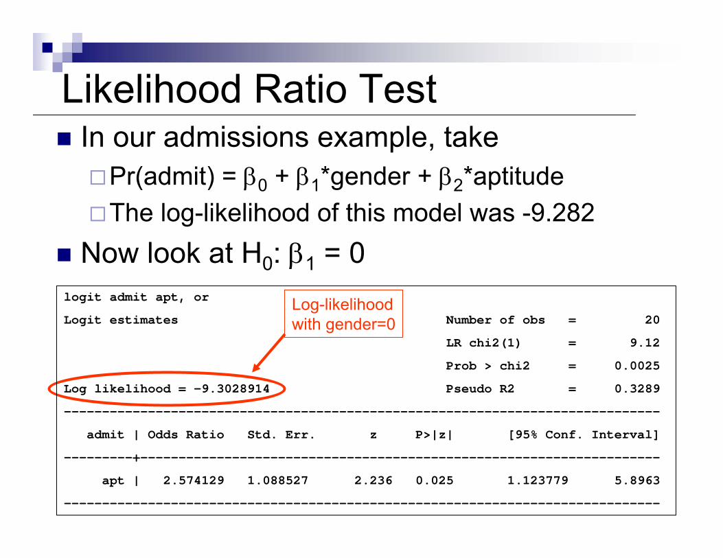
Likelihood Ratio TestIn our admissions example, take
Pr(admit) = β0 + β1*gender + β2*aptitudeThe log-likelihood of this model was -9.282
Now look at H0: β1 = 0The likelihood of the regression with gender but not aptitude was -9.303
Likelihood ratio test:[-2 * (-9.303)] – [-2 * (-9.282)] = 0.042From Stata
dis 1- chi2(1, .042).83761977
Not significant at 5% level. Therefore we fail to reject the null hypothesis that β1 = 0.
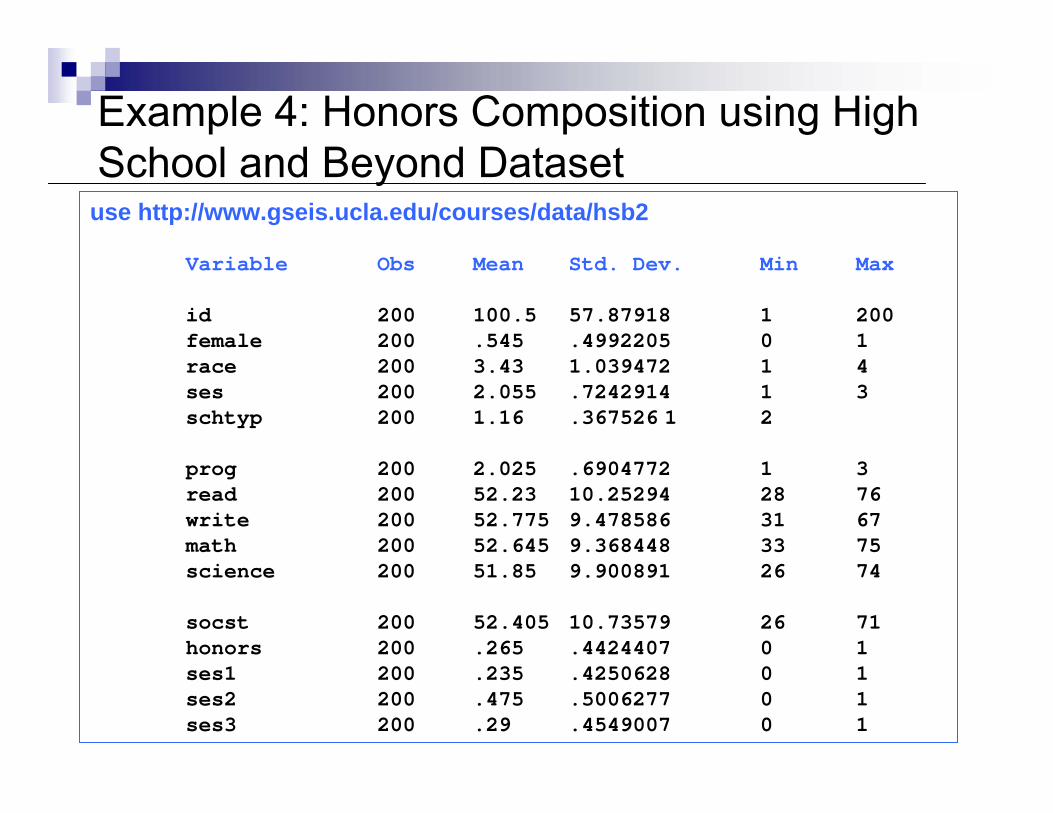
Example 4: Honors Composition using High School and Beyond Dataset
use http://www.gseis.ucla.edu/courses/data/hsb2
Variable Obs Mean Std. Dev. Min Max
id 200 100.5 57.87918 1 200female 200 .545 .4992205 0 1race 200 3.43 1.039472 1 4ses 200 2.055 .7242914 1 3schtyp 200 1.16 .367526 1 2
prog 200 2.025 .6904772 1 3read 200 52.23 10.25294 28 76write 200 52.775 9.478586 31 67math 200 52.645 9.368448 33 75science 200 51.85 9.900891 26 74
socst 200 52.405 10.73579 26 71honors 200 .265 .4424407 0 1ses1 200 .235 .4250628 0 1ses2 200 .475 .5006277 0 1ses3 200 .29 .4549007 0 1
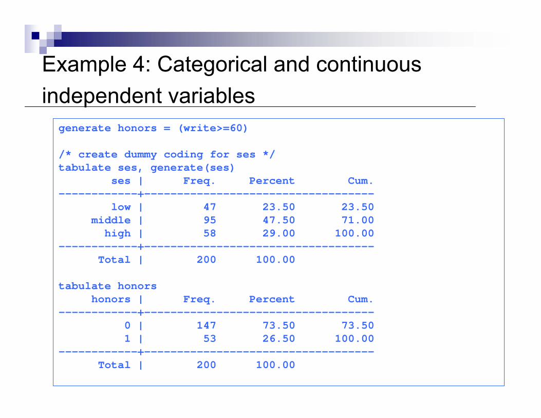
Example 4: Categorical and continuous independent variables
generate honors = (write>=60)
/* create dummy coding for ses */tabulate ses, generate(ses)
ses | Freq. Percent Cum.------------+-----------------------------------
low | 47 23.50 23.50middle | 95 47.50 71.00
high | 58 29.00 100.00------------+-----------------------------------
Total | 200 100.00
tabulate honorshonors | Freq. Percent Cum.
------------+-----------------------------------0 | 147 73.50 73.501 | 53 26.50 100.00
------------+-----------------------------------Total | 200 100.00
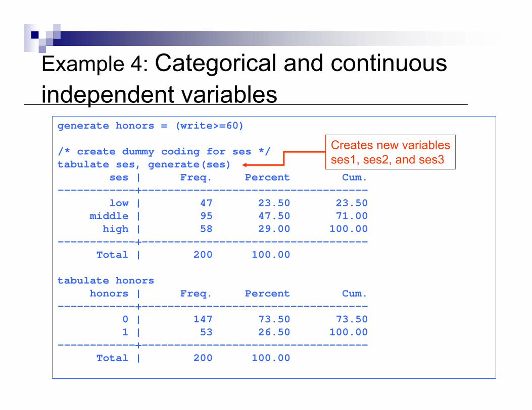
Creates new variablesses1, ses2, and ses3
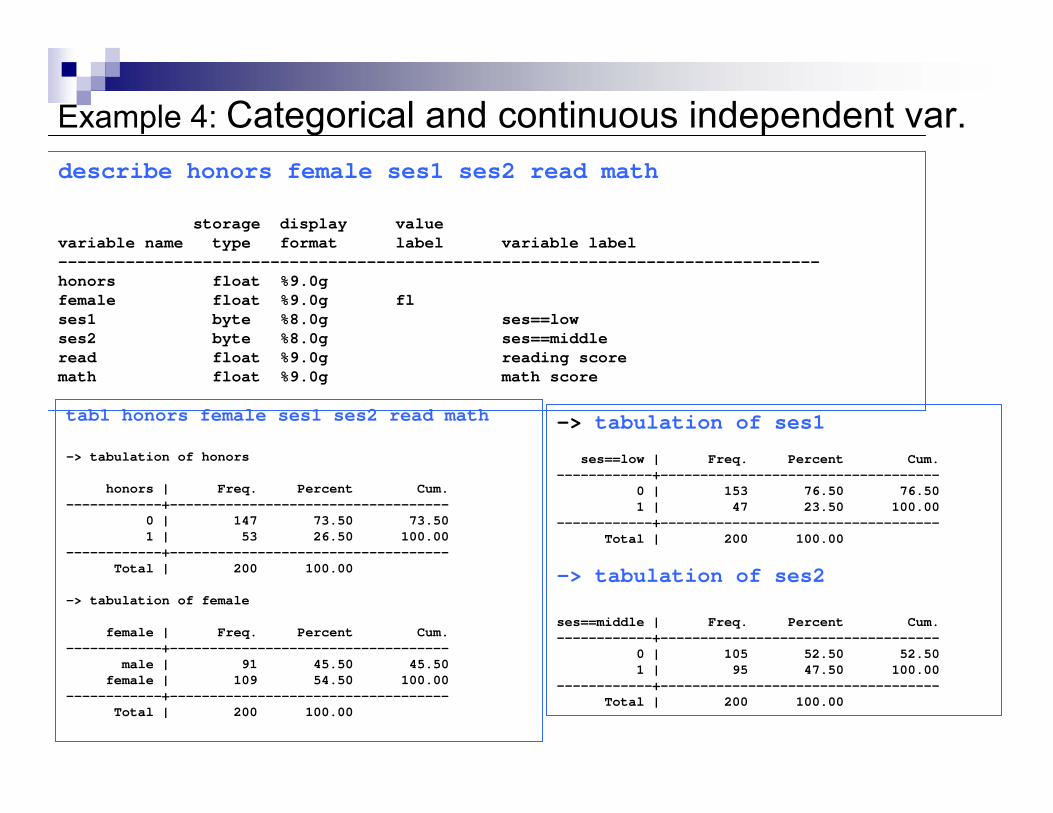
Example 4: Categorical and continuous independent var.describe honors female ses1 ses2 read math
storage display valuevariable name type format label variable label-------------------------------------------------------------------------------honors float %9.0g female float %9.0g fl ses1 byte %8.0g ses==lowses2 byte %8.0g ses==middleread float %9.0g reading scoremath float %9.0g math score
tab1 honors female ses1 ses2 read math
-> tabulation of honors
honors | Freq. Percent Cum.------------+-----------------------------------
0 | 147 73.50 73.501 | 53 26.50 100.00
------------+-----------------------------------Total | 200 100.00
-> tabulation of female
female | Freq. Percent Cum.------------+-----------------------------------
male | 91 45.50 45.50female | 109 54.50 100.00
------------+-----------------------------------Total | 200 100.00
-> tabulation of ses1
ses==low | Freq. Percent Cum.------------+-----------------------------------
0 | 153 76.50 76.501 | 47 23.50 100.00
------------+-----------------------------------Total | 200 100.00
-> tabulation of ses2
ses==middle | Freq. Percent Cum.------------+-----------------------------------
0 | 105 52.50 52.501 | 95 47.50 100.00
------------+-----------------------------------Total | 200 100.00
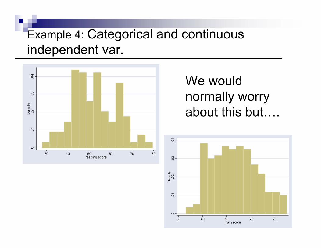
Example 4: Categorical and continuous independent var.
0.0
1.0
2.0
3.0
4D
ensi
ty
30 40 50 60 70 80reading score
0.0
1.0
2.0
3.0
4D
ensi
ty
30 40 50 60 70math score
We would normally worry about this but….
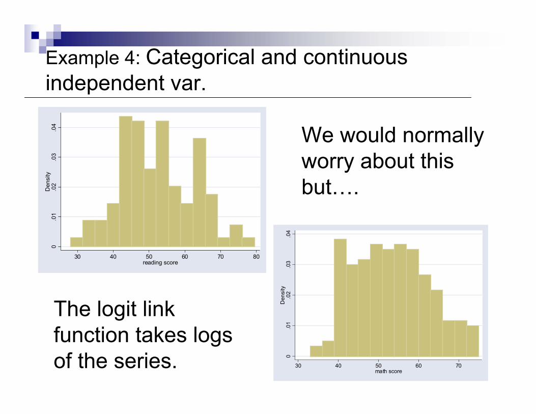
Example 4: Categorical and continuous independent var.
0.0
1.0
2.0
3.0
4D
ensi
ty
30 40 50 60 70 80reading score
0.0
1.0
2.0
3.0
4D
ensi
ty
30 40 50 60 70math score
We would normally worry about this but….
The logit link function takes logs of the series.
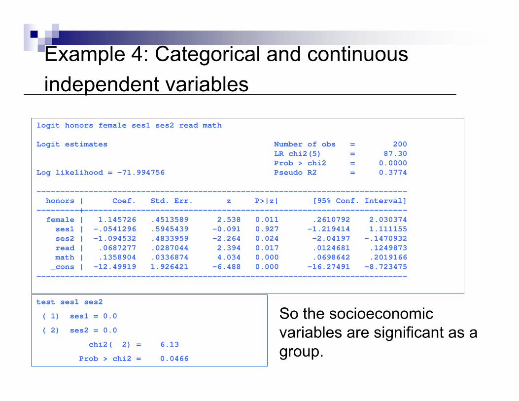
Example 4: Categorical and continuous independent variables
logit honors female ses1 ses2 read math
Logit estimates Number of obs = 200LR chi2(5) = 87.30Prob > chi2 = 0.0000
Log likelihood = -71.994756 Pseudo R2 = 0.3774
------------------------------------------------------------------------------honors | Coef. Std. Err. z P>|z| [95% Conf. Interval]
---------+--------------------------------------------------------------------female | 1.145726 .4513589 2.538 0.011 .2610792 2.030374
ses1 | -.0541296 .5945439 -0.091 0.927 -1.219414 1.111155ses2 | -1.094532 .4833959 -2.264 0.024 -2.04197 -.1470932read | .0687277 .0287044 2.394 0.017 .0124681 .1249873math | .1358904 .0336874 4.034 0.000 .0698642 .2019166
_cons | -12.49919 1.926421 -6.488 0.000 -16.27491 -8.723475------------------------------------------------------------------------------
test ses1 ses2
( 1) ses1 = 0.0
( 2) ses2 = 0.0
chi2( 2) = 6.13
Prob > chi2 = 0.0466
So the socioeconomic variables are significant as a group.
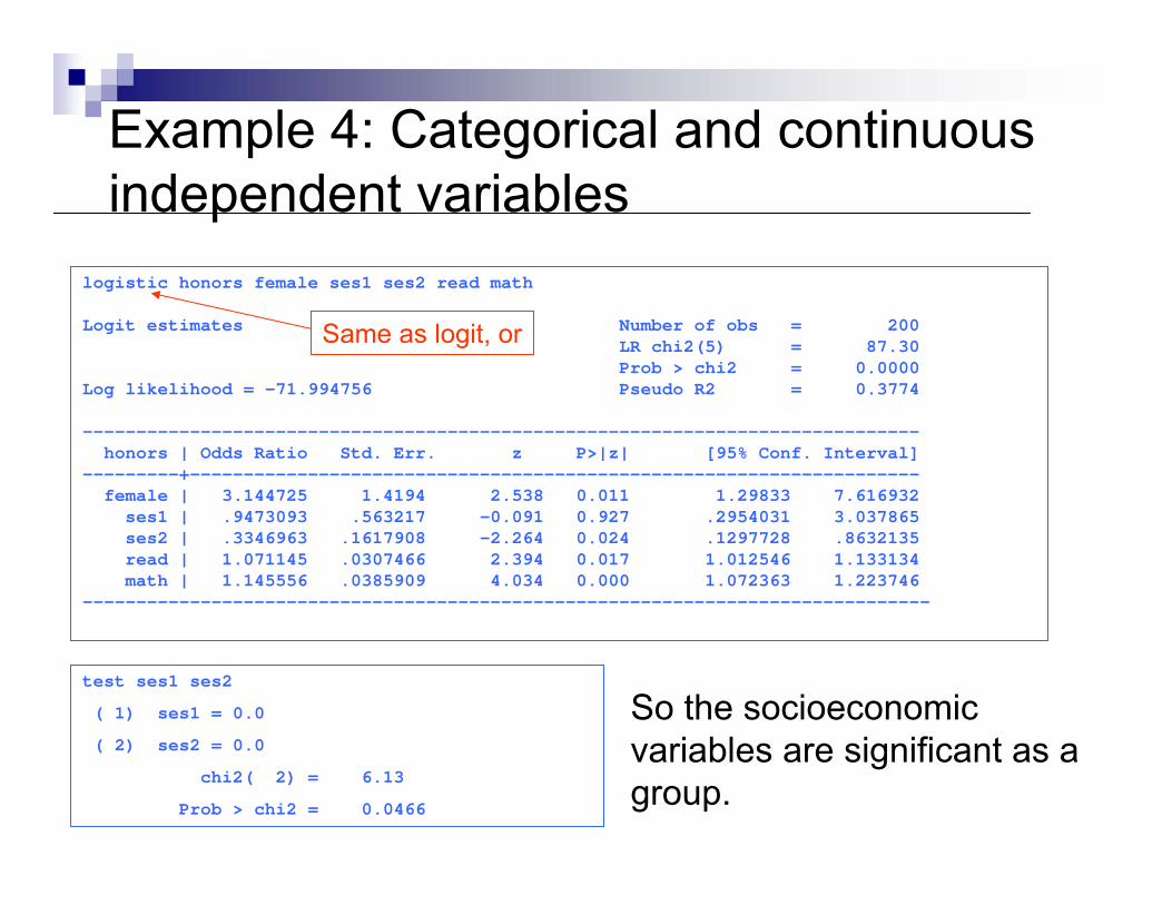
logistic honors female ses1 ses2 read math
Logit estimates Number of obs = 200LR chi2(5) = 87.30Prob > chi2 = 0.0000
Log likelihood = -71.994756 Pseudo R2 = 0.3774
------------------------------------------------------------------------------honors | Odds Ratio Std. Err. z P>|z| [95% Conf. Interval]
---------+--------------------------------------------------------------------female | 3.144725 1.4194 2.538 0.011 1.29833 7.616932
ses1 | .9473093 .563217 -0.091 0.927 .2954031 3.037865ses2 | .3346963 .1617908 -2.264 0.024 .1297728 .8632135read | 1.071145 .0307466 2.394 0.017 1.012546 1.133134math | 1.145556 .0385909 4.034 0.000 1.072363 1.223746
-------------------------------------------------------------------------------
test ses1 ses2
( 1) ses1 = 0.0
( 2) ses2 = 0.0
chi2( 2) = 6.13
Prob > chi2 = 0.0466
Example 4: Categorical and continuous independent variables
So the socioeconomic variables are significant as a group.
Same as logit, or
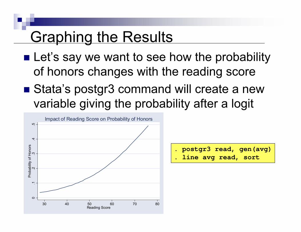
Graphing the ResultsLet’s say we want to see how the probability of honors changes with the reading scoreStata’s postgr3 command will create a new variable giving the probability after a logit
0.1
.2.3
.4.5
Pro
babi
lity
of H
onor
s
30 40 50 60 70 80Reading Score
Impact of Reading Score on Probability of Honors
. postgr3 read, gen(avg)
. line avg read, sort
0.2
.4.6
Pro
babi
lity
of H
onor
s
30 40 50 60 70 80Reading Score
Average Male Female
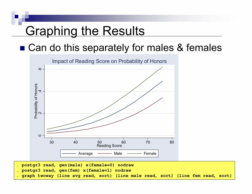
Impact of Reading Score on Probability of Honors
Graphing the ResultsCan do this separately for males & females
. postgr3 read, gen(male) x(female=0) nodraw
. postgr3 read, gen(fem) x(female=1) nodraw
. graph twoway (line avg read, sort) (line male read, sort) (line fem read, sort)
0.2
.4.6
Pro
babi
lity
of H
onor
s
30 40 50 60 70 80Reading Score
Average Male Female
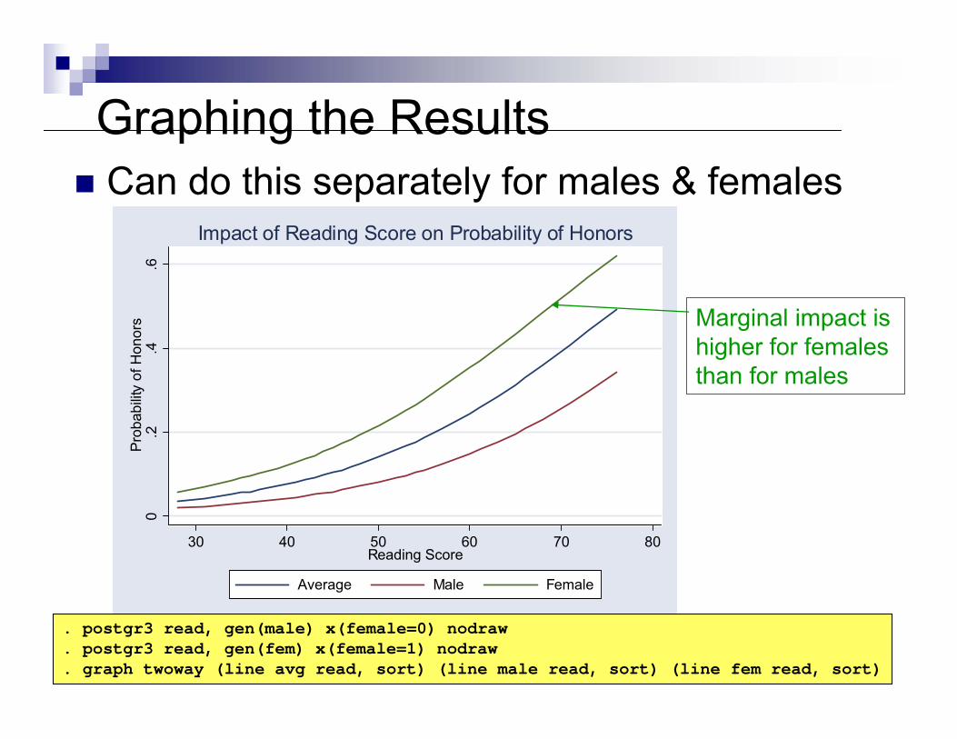
Impact of Reading Score on Probability of Honors
Graphing the ResultsCan do this separately for males & females
. postgr3 read, gen(male) x(female=0) nodraw
. postgr3 read, gen(fem) x(female=1) nodraw
. graph twoway (line avg read, sort) (line male read, sort) (line fem read, sort)
Marginal impact ishigher for females than for males
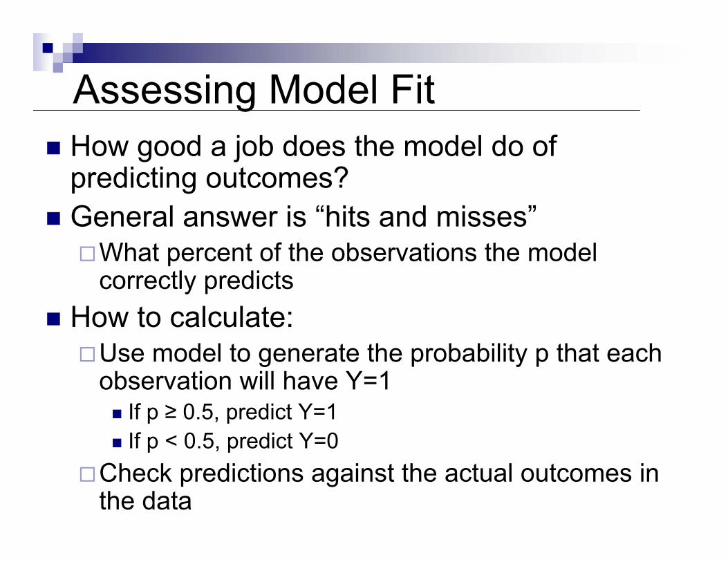
Assessing Model FitHow good a job does the model do of predicting outcomes?General answer is “hits and misses”
What percent of the observations the model correctly predicts
How to calculate:Use model to generate the probability p that each observation will have Y=1
If p ≥ 0.5, predict Y=1If p < 0.5, predict Y=0
Check predictions against the actual outcomes in the data
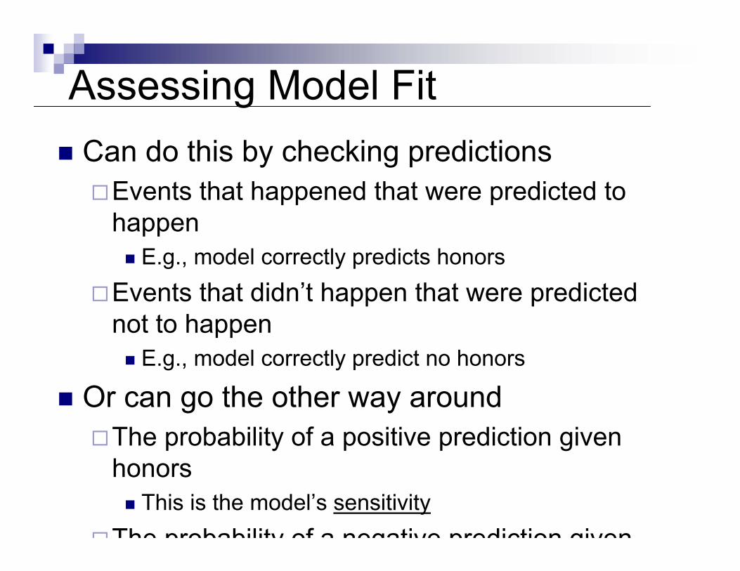
Assessing Model FitCan do this by checking predictions
Events that happened that were predicted to happen
E.g., model correctly predicts honorsEvents that didn’t happen that were predicted not to happen
E.g., model correctly predict no honors
Or can go the other way aroundThe probability of a positive prediction given honors
This is the model’s sensitivityThe probability of a negative prediction given
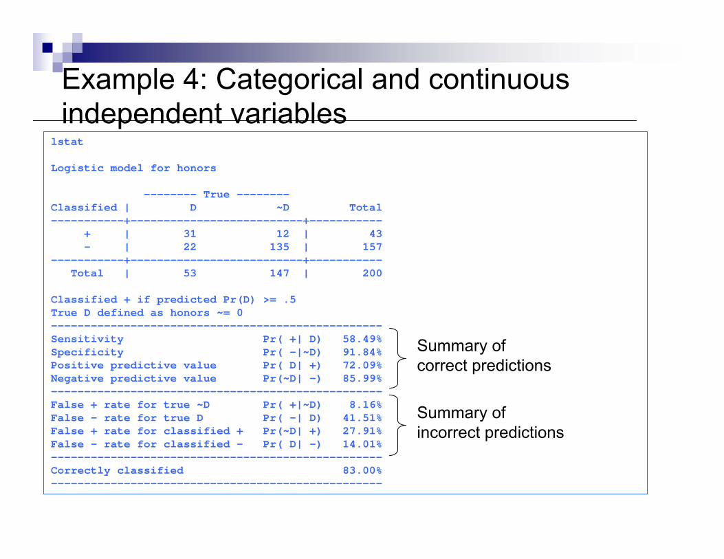
Example 4: Categorical and continuous independent variables
lstat
Logistic model for honors
-------- True --------Classified | D ~D Total-----------+--------------------------+-----------
+ | 31 12 | 43- | 22 135 | 157
-----------+--------------------------+-----------Total | 53 147 | 200
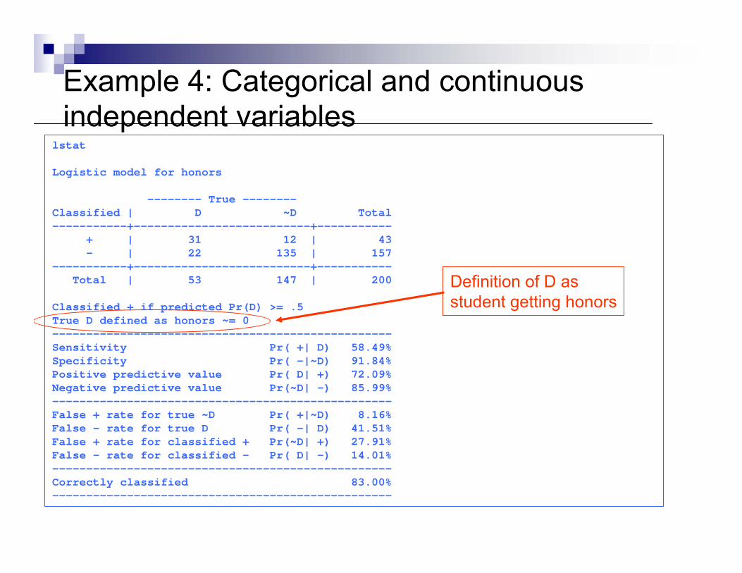
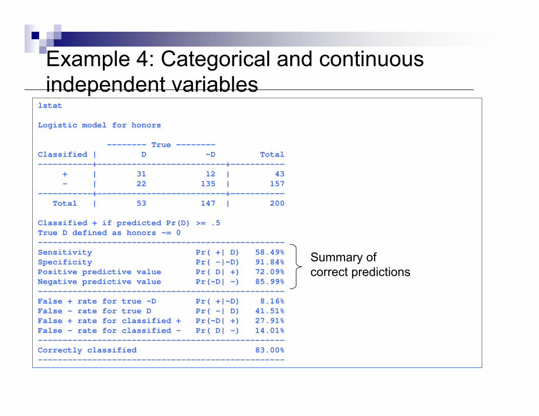
Classified + if predicted Pr(D) >= .5True D defined as honors ~= 0--------------------------------------------------Sensitivity Pr( +| D) 58.49%Specificity Pr( -|~D) 91.84%Positive predictive value Pr( D| +) 72.09%Negative predictive value Pr(~D| -) 85.99%--------------------------------------------------False + rate for true ~D Pr( +|~D) 8.16%False - rate for true D Pr( -| D) 41.51%False + rate for classified + Pr(~D| +) 27.91%False - rate for classified - Pr( D| -) 14.01%--------------------------------------------------Correctly classified 83.00%--------------------------------------------------
Definition of D asstudent getting honors
lstat
Logistic model for honors
-------- True --------Classified | D ~D Total-----------+--------------------------+-----------
+ | 31 12 | 43- | 22 135 | 157
-----------+--------------------------+-----------Total | 53 147 | 200
Classified + if predicted Pr(D) >= .5True D defined as honors ~= 0--------------------------------------------------Sensitivity Pr( +| D) 58.49%Specificity Pr( -|~D) 91.84%Positive predictive value Pr( D| +) 72.09%Negative predictive value Pr(~D| -) 85.99%--------------------------------------------------False + rate for true ~D Pr( +|~D) 8.16%False - rate for true D Pr( -| D) 41.51%False + rate for classified + Pr(~D| +) 27.91%False - rate for classified - Pr( D| -) 14.01%--------------------------------------------------Correctly classified 83.00%--------------------------------------------------
Summary ofcorrect predictions
Example 4: Categorical and continuous independent variables
lstat
Logistic model for honors
-------- True --------Classified | D ~D Total-----------+--------------------------+-----------
+ | 31 12 | 43- | 22 135 | 157
-----------+--------------------------+-----------Total | 53 147 | 200
Classified + if predicted Pr(D) >= .5True D defined as honors ~= 0--------------------------------------------------Sensitivity Pr( +| D) 58.49%Specificity Pr( -|~D) 91.84%Positive predictive value Pr( D| +) 72.09%Negative predictive value Pr(~D| -) 85.99%--------------------------------------------------False + rate for true ~D Pr( +|~D) 8.16%False - rate for true D Pr( -| D) 41.51%False + rate for classified + Pr(~D| +) 27.91%False - rate for classified - Pr( D| -) 14.01%--------------------------------------------------Correctly classified 83.00%--------------------------------------------------
Summary ofcorrect predictions
Summary ofincorrect predictions
Example 4: Categorical and continuous independent variables
lstat
Logistic model for honors
-------- True --------Classified | D ~D Total-----------+--------------------------+-----------
+ | 31 12 | 43- | 22 135 | 157
-----------+--------------------------+-----------Total | 53 147 | 200
Classified + if predicted Pr(D) >= .5True D defined as honors ~= 0--------------------------------------------------Sensitivity Pr( +| D) 58.49%Specificity Pr( -|~D) 91.84%Positive predictive value Pr( D| +) 72.09%Negative predictive value Pr(~D| -) 85.99%--------------------------------------------------False + rate for true ~D Pr( +|~D) 8.16%False - rate for true D Pr( -| D) 41.51%False + rate for classified + Pr(~D| +) 27.91%False - rate for classified - Pr( D| -) 14.01%--------------------------------------------------Correctly classified 83.00%--------------------------------------------------
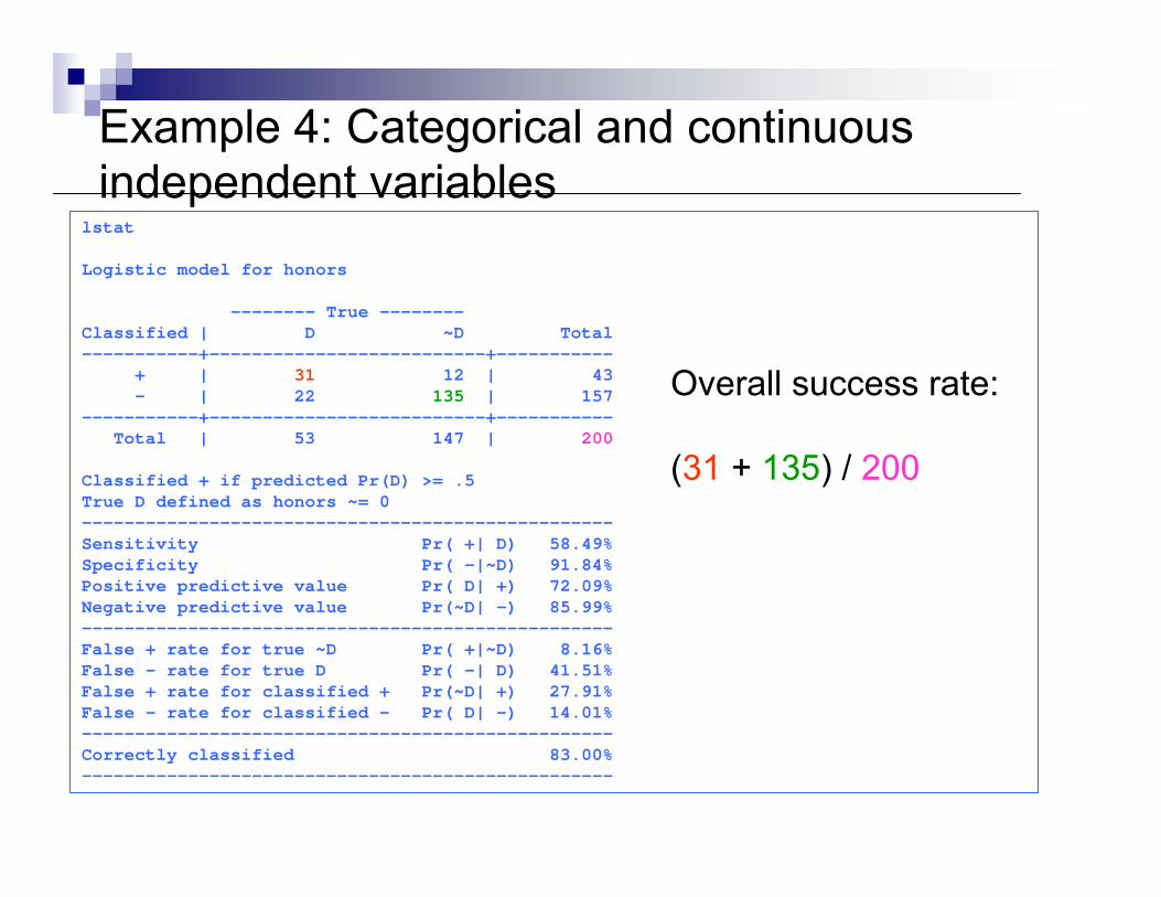
Overall success rate:
(31 + 135) / 200
Example 4: Categorical and continuous independent variables
lstat
Logistic model for honors
-------- True --------Classified | D ~D Total-----------+--------------------------+-----------
+ | 31 12 | 43- | 22 135 | 157
-----------+--------------------------+-----------Total | 53 147 | 200
Classified + if predicted Pr(D) >= .5True D defined as honors ~= 0--------------------------------------------------Sensitivity Pr( +| D) 58.49%Specificity Pr( -|~D) 91.84%Positive predictive value Pr( D| +) 72.09%Negative predictive value Pr(~D| -) 85.99%--------------------------------------------------False + rate for true ~D Pr( +|~D) 8.16%False - rate for true D Pr( -| D) 41.51%False + rate for classified + Pr(~D| +) 27.91%False - rate for classified - Pr( D| -) 14.01%--------------------------------------------------Correctly classified 83.00%--------------------------------------------------
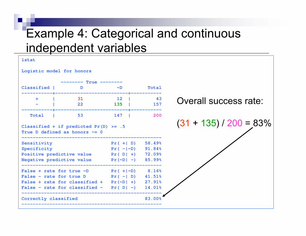
Overall success rate:
(31 + 135) / 200 = 83%
Example 4: Categorical and continuous independent variables
Assessing Model FitThis is all calculated using 50% as a cutoff point for positive predictionsBut this isn’t set in stone; depending on your application, you might want to change itYou might want to avoid false positives
For example, don’t convict innocent peopleThen you would set the cutoff higher than 50%
Or you might want to avoid false negativesFor example, don’t report that someone who has a disease is actually healthyThen you would set the cutoff lower than 50%
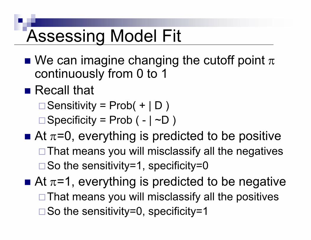
Assessing Model FitWe can imagine changing the cutoff point πcontinuously from 0 to 1Recall that
Sensitivity = Prob( + | D )Specificity = Prob ( - | ~D )
At π=0, everything is predicted to be positiveThat means you will misclassify all the negativesSo the sensitivity=1, specificity=0
At π=1, everything is predicted to be negativeThat means you will misclassify all the positivesSo the sensitivity=0, specificity=1
Assessing Model FitIn between, you can vary the number of false positives and false negatives
If your model does a good job of predicting outcomes, these should be low for all π
The ROC curve plots the sensitivity and 1-specificity as π goes from 0 to 1
The better the model does at predicting, the greater will be the area under the ROC curve
Produce these with Stata command “lroc”
Example 4: Categorical and continuous independent variables
0.00
0.25
0.50
0.75
1.00
Sen
sitiv
ity
0.00 0.25 0.50 0.75 1.001 - Specificity
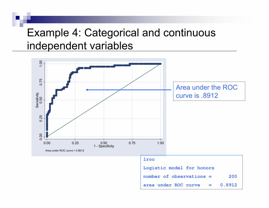
Area under ROC curve = 0.8912
lroc
Logistic model for honors
number of observations = 200
area under ROC curve = 0.8912
Area under the ROC curve is .8912
Example 4: Categorical and continuous independent variables
0.00
0.25
0.50
0.75
1.00
Sen
sitiv
ity/S
peci
ficity
0.00 0.25 0.50 0.75 1.00Probability cutoff
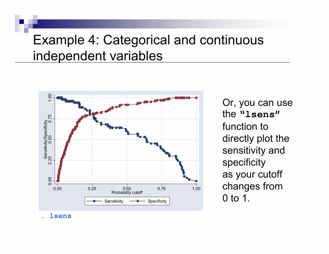
Sensitivity Specificity
. lsens
Or, you can use the “lsens”function to directly plot the sensitivity and specificityas your cutoff changes from0 to 1.
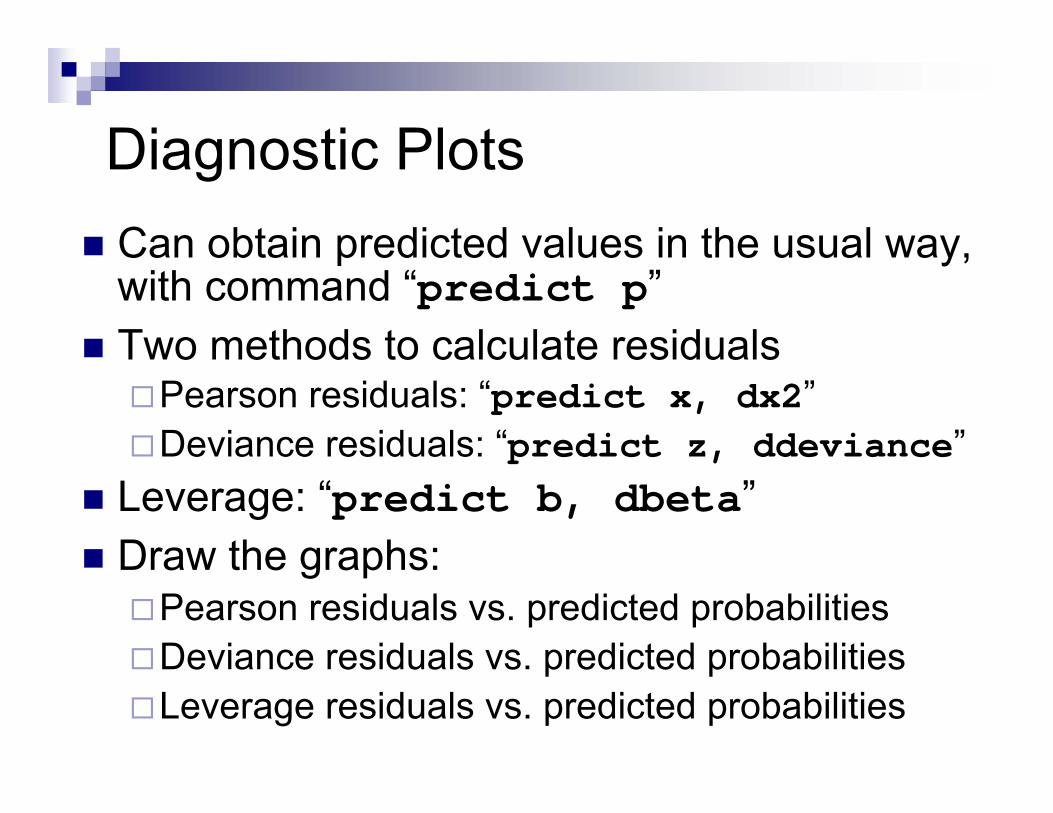
Diagnostic PlotsCan obtain predicted values in the usual way, with command “predict p”Two methods to calculate residuals
Pearson residuals: “predict x, dx2”Deviance residuals: “predict z, ddeviance”
Leverage: “predict b, dbeta”Draw the graphs:
Pearson residuals vs. predicted probabilitiesDeviance residuals vs. predicted probabilitiesLeverage residuals vs. predicted probabilities
Diagnostic Plots0
1020
30H
-L d
X^2
0 .2 .4 .6 .8 1Pr(honors)
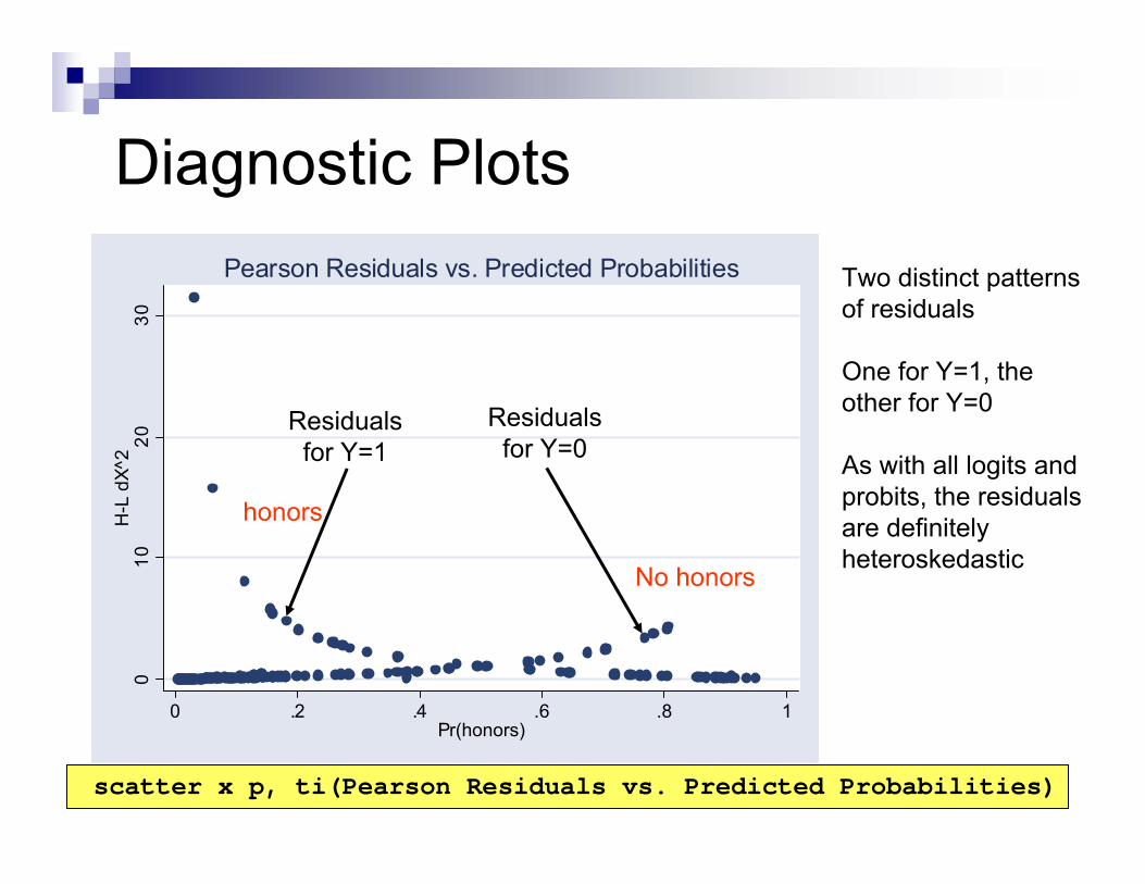
Pearson Residuals vs. Predicted Probabilities
Residualsfor Y=1
Two distinct patternsof residuals
One for Y=1, the other for Y=0
As with all logits andprobits, the residualsare definitelyheteroskedastic
scatter x p, ti(Pearson Residuals vs. Predicted Probabilities)
Residualsfor Y=0
honors
No honors
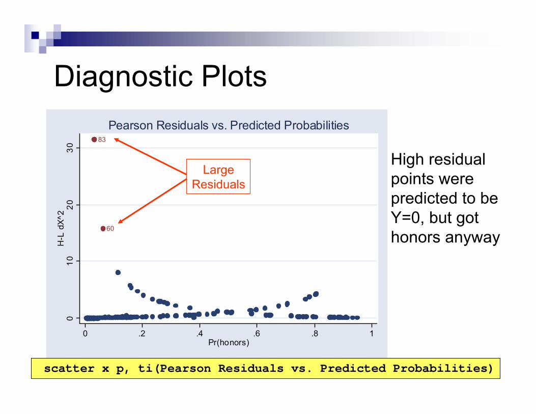
60
83
010
2030
H-L
dX^
2
0 .2 .4 .6 .8 1Pr(honors)
Pearson Residuals vs. Predicted Probabilities
Diagnostic Plots
LargeResiduals
High residual points were predicted to be Y=0, but got honors anyway
scatter x p, ti(Pearson Residuals vs. Predicted Probabilities)
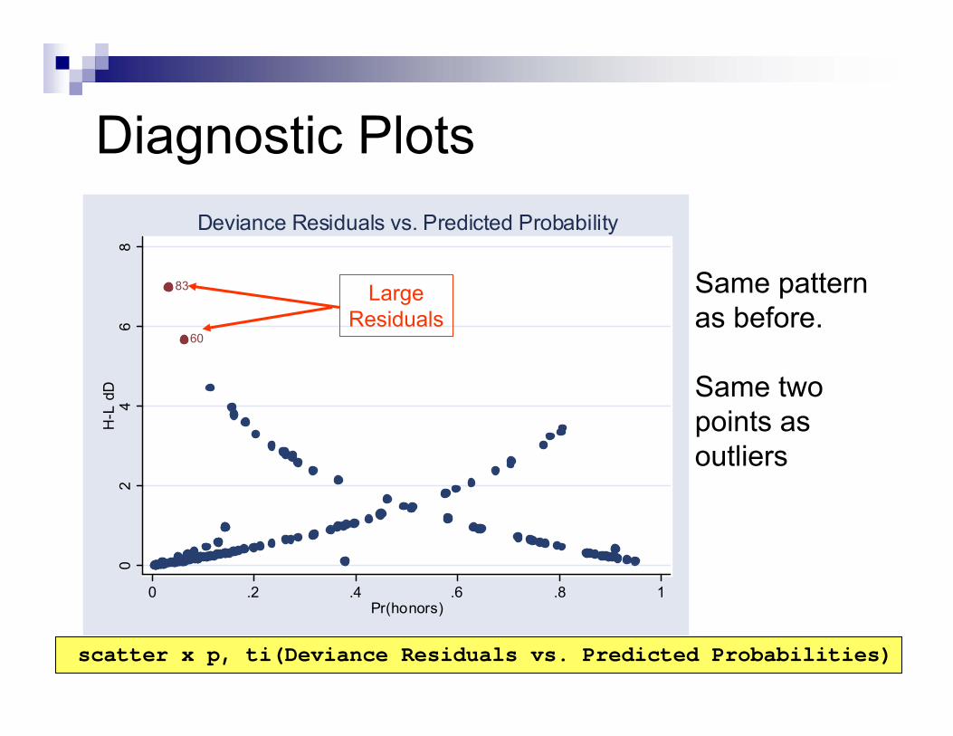
60
83
02
46
8H
-L d
D
0 .2 .4 .6 .8 1Pr(honors)
Deviance Residuals vs. Predicted Probability
Diagnostic Plots
LargeResiduals
Same pattern as before.
Same two points as outliers
scatter x p, ti(Deviance Residuals vs. Predicted Probabilities)
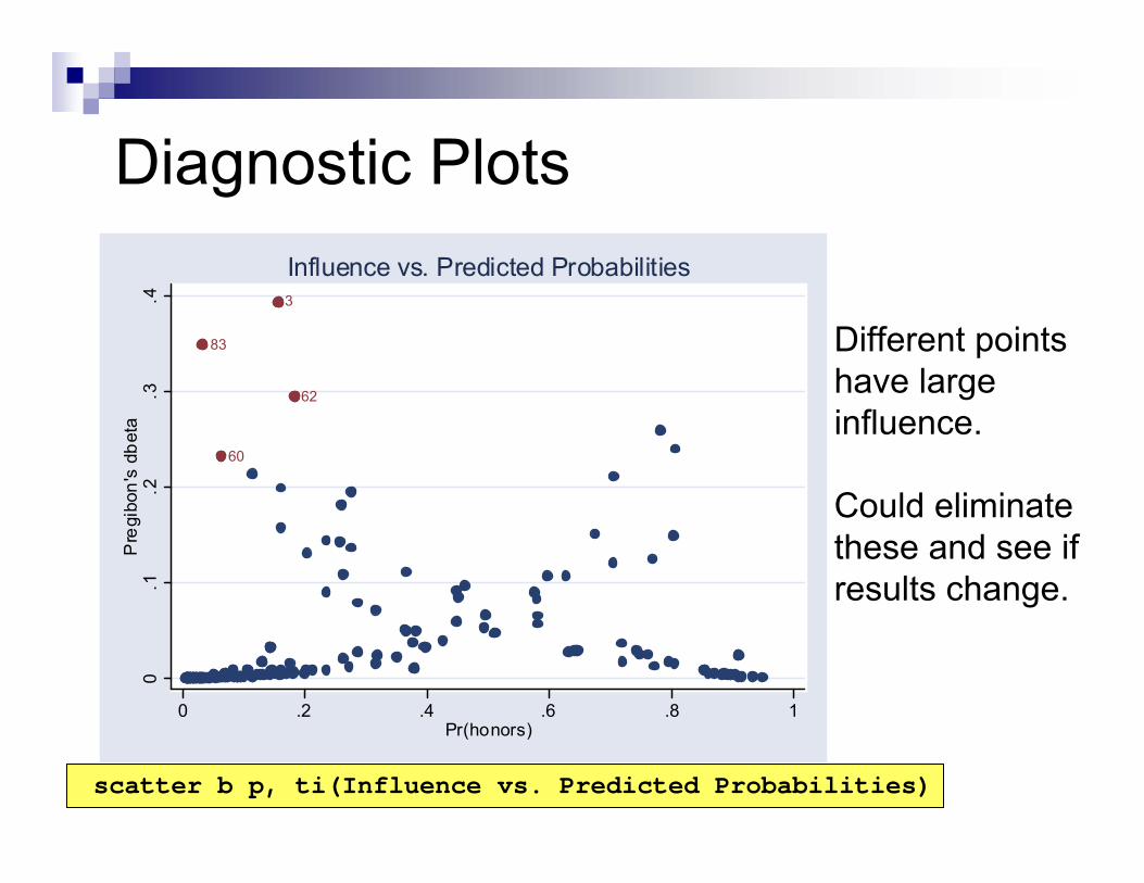
62
3
60
83
0.1
.2.3
.4P
regi
bon'
s db
eta
0 .2 .4 .6 .8 1Pr(honors)
Influence vs. Predicted Probabilities
Diagnostic Plots
scatter b p, ti(Influence vs. Predicted Probabilities)
Different points have large influence.
Could eliminate these and see if results change.
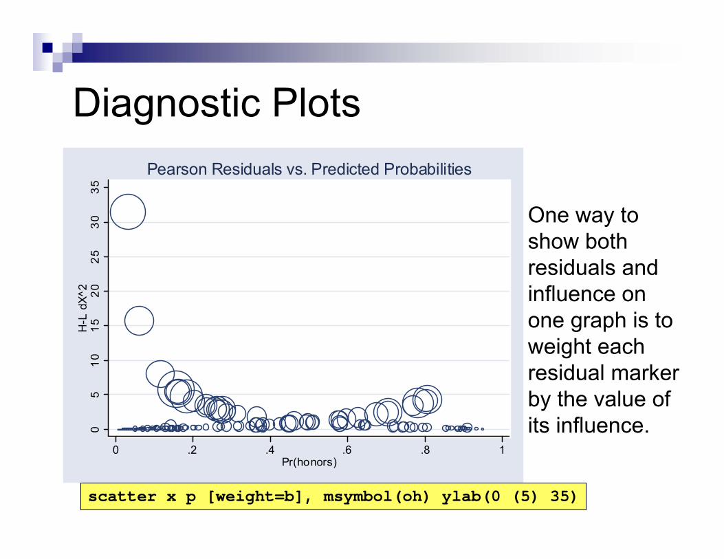
05
1015
2025
3035
H-L
dX^
2
0 .2 .4 .6 .8 1Pr(honors)
Pearson Residuals vs. Predicted Probabilities
Diagnostic Plots
One way to show both residuals and influence on one graph is to weight each residual marker by the value of its influence.
scatter x p [weight=b], msymbol(oh) ylab(0 (5) 35)
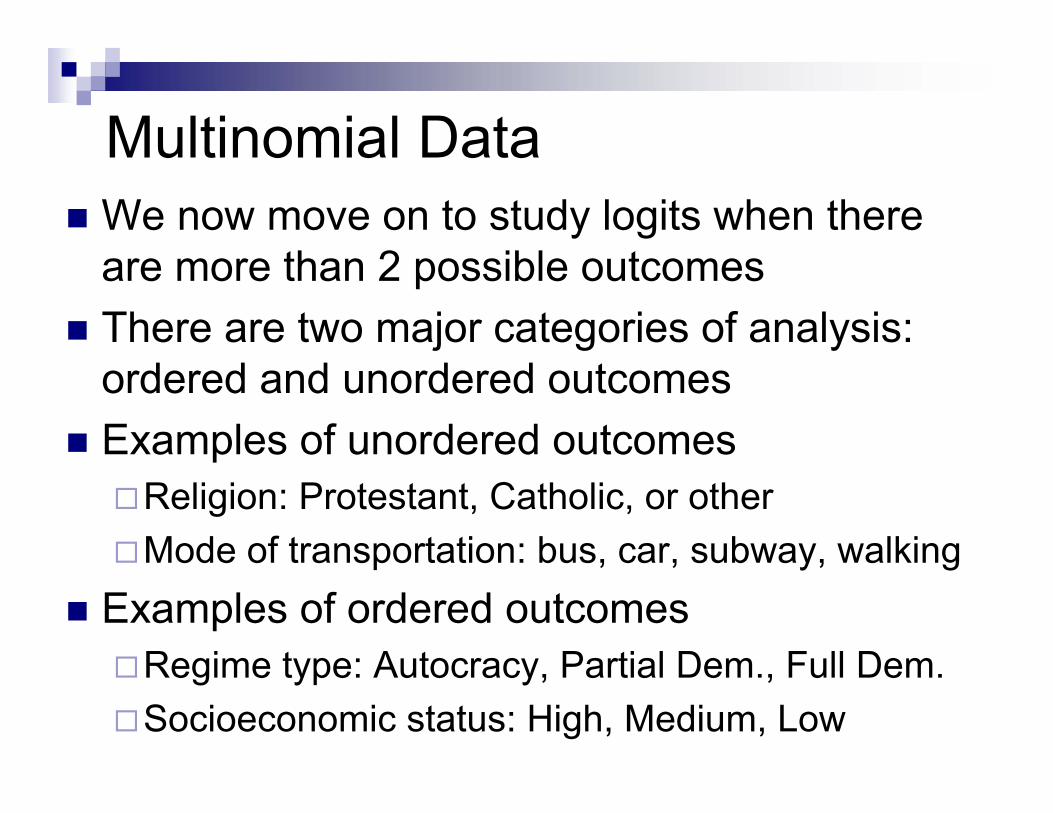
Multinomial DataWe now move on to study logits when there are more than 2 possible outcomesThere are two major categories of analysis: ordered and unordered outcomesExamples of unordered outcomes
Religion: Protestant, Catholic, or otherMode of transportation: bus, car, subway, walking
Examples of ordered outcomesRegime type: Autocracy, Partial Dem., Full Dem.Socioeconomic status: High, Medium, Low
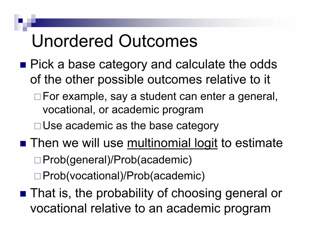
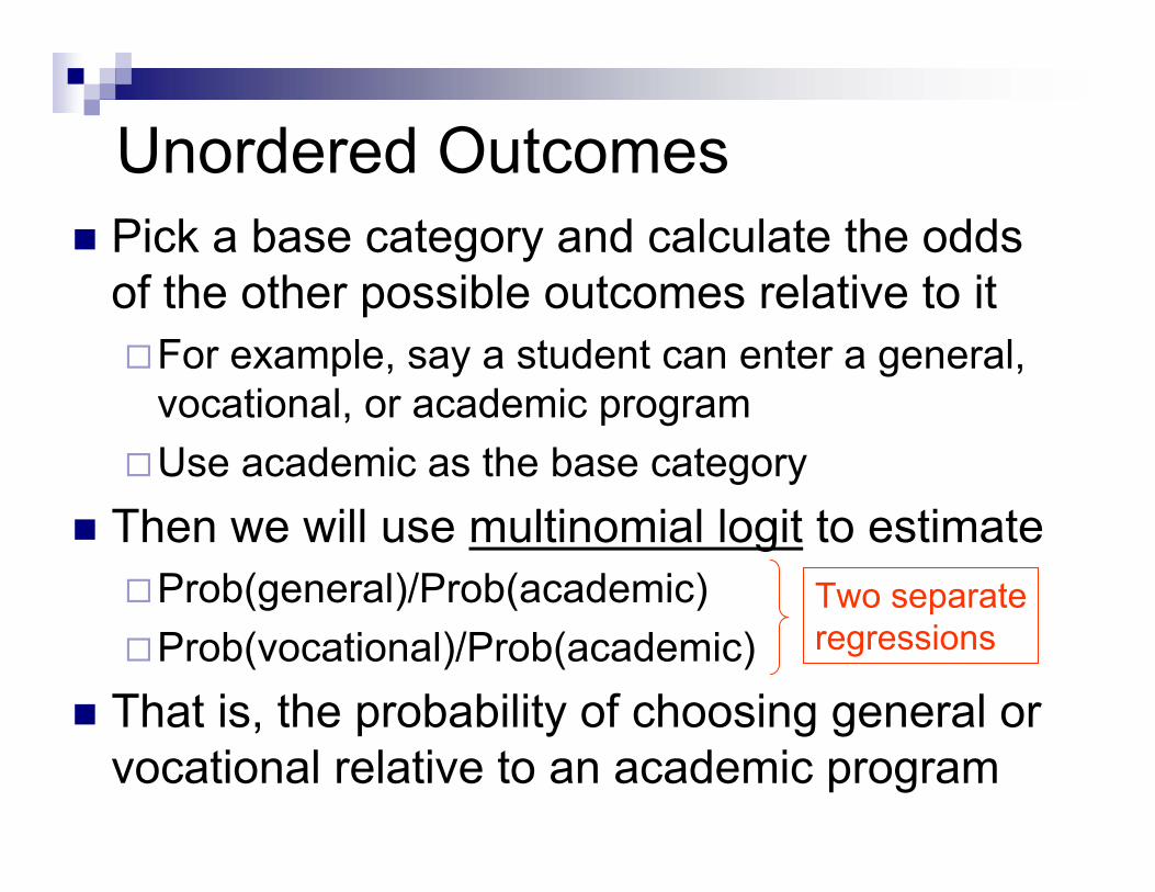
Unordered OutcomesPick a base category and calculate the odds of the other possible outcomes relative to it
For example, say a student can enter a general, vocational, or academic programUse academic as the base category
Then we will use multinomial logit to estimateProb(general)/Prob(academic)Prob(vocational)/Prob(academic)
That is, the probability of choosing general or vocational relative to an academic program
Two separateregressions
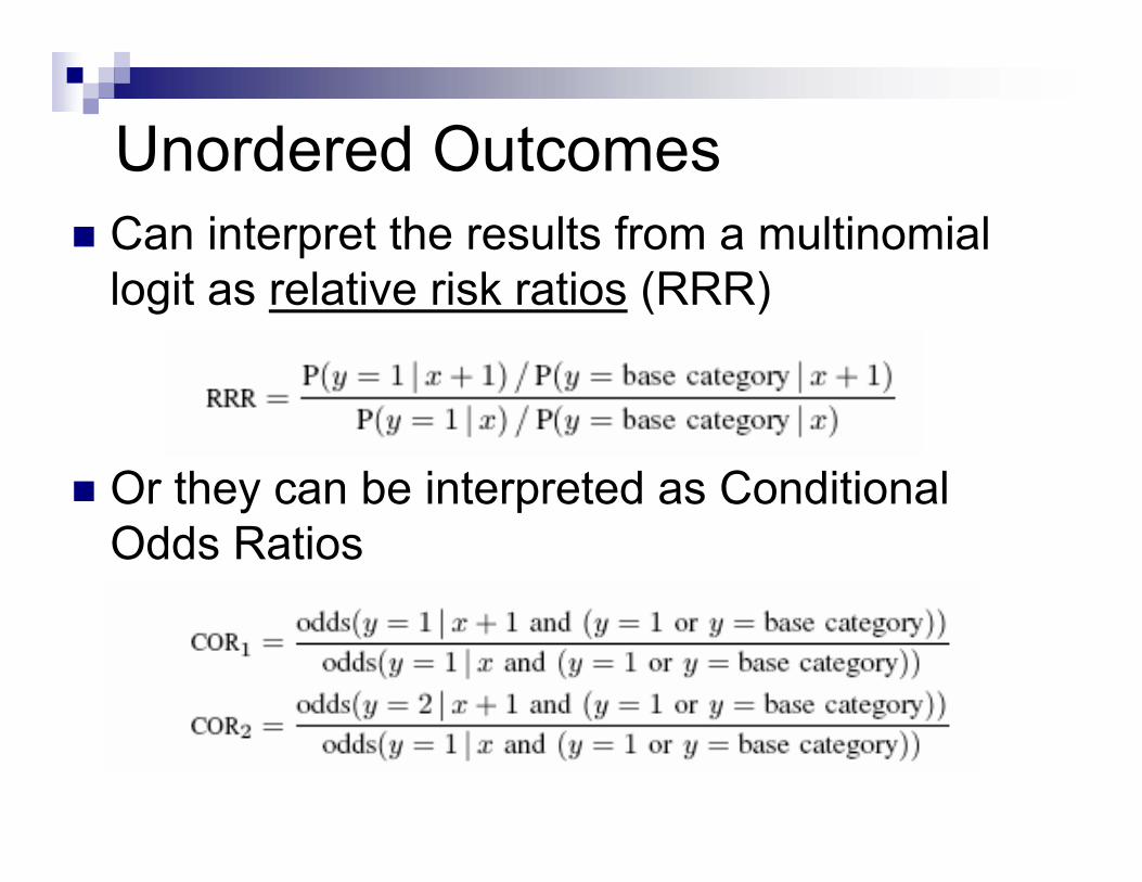
Can interpret the results from a multinomial logit as relative risk ratios (RRR)
Or they can be interpreted as Conditional Odds Ratios
Unordered Outcomes
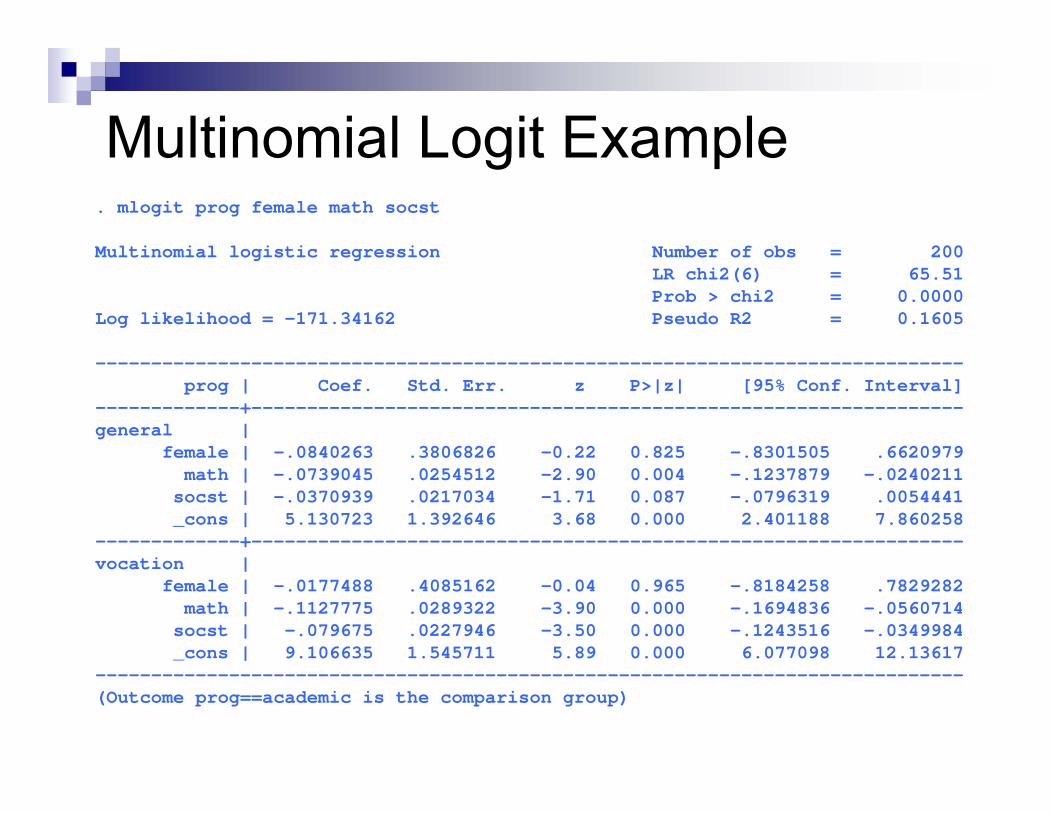
Multinomial Logit Example. mlogit prog female math socst
Multinomial logistic regression Number of obs = 200LR chi2(6) = 65.51Prob > chi2 = 0.0000
Log likelihood = -171.34162 Pseudo R2 = 0.1605
------------------------------------------------------------------------------prog | Coef. Std. Err. z P>|z| [95% Conf. Interval]
-------------+----------------------------------------------------------------general |
female | -.0840263 .3806826 -0.22 0.825 -.8301505 .6620979math | -.0739045 .0254512 -2.90 0.004 -.1237879 -.0240211
socst | -.0370939 .0217034 -1.71 0.087 -.0796319 .0054441_cons | 5.130723 1.392646 3.68 0.000 2.401188 7.860258
-------------+----------------------------------------------------------------vocation |
female | -.0177488 .4085162 -0.04 0.965 -.8184258 .7829282math | -.1127775 .0289322 -3.90 0.000 -.1694836 -.0560714
socst | -.079675 .0227946 -3.50 0.000 -.1243516 -.0349984_cons | 9.106635 1.545711 5.89 0.000 6.077098 12.13617
------------------------------------------------------------------------------(Outcome prog==academic is the comparison group)
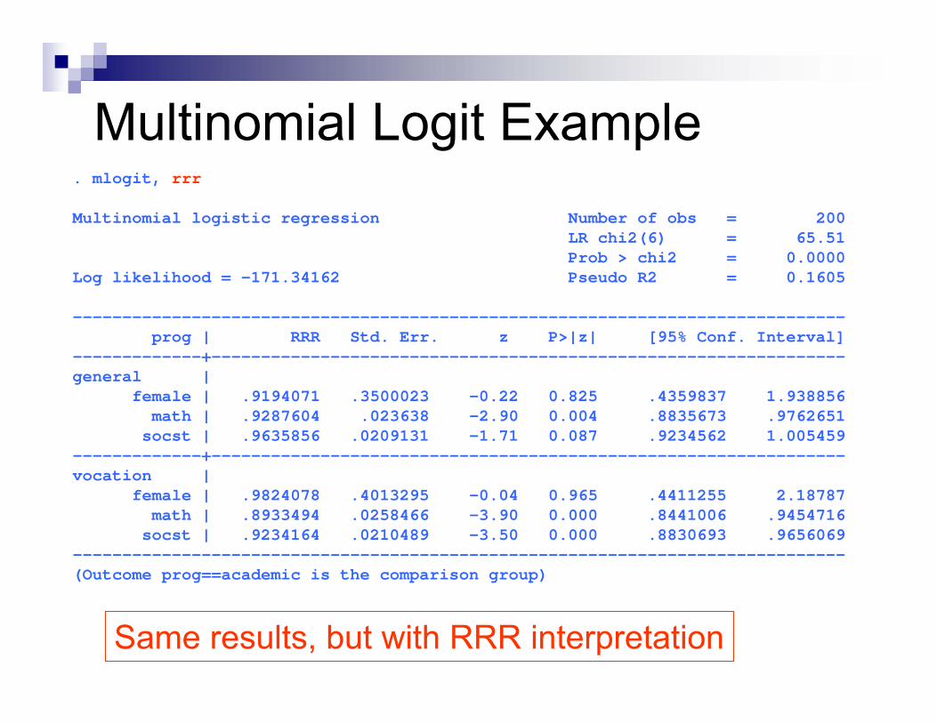
Multinomial Logit Example. mlogit, rrr
Multinomial logistic regression Number of obs = 200LR chi2(6) = 65.51Prob > chi2 = 0.0000
Log likelihood = -171.34162 Pseudo R2 = 0.1605
------------------------------------------------------------------------------prog | RRR Std. Err. z P>|z| [95% Conf. Interval]
-------------+----------------------------------------------------------------general |
female | .9194071 .3500023 -0.22 0.825 .4359837 1.938856math | .9287604 .023638 -2.90 0.004 .8835673 .9762651
socst | .9635856 .0209131 -1.71 0.087 .9234562 1.005459-------------+----------------------------------------------------------------vocation |
female | .9824078 .4013295 -0.04 0.965 .4411255 2.18787math | .8933494 .0258466 -3.90 0.000 .8441006 .9454716
socst | .9234164 .0210489 -3.50 0.000 .8830693 .9656069------------------------------------------------------------------------------(Outcome prog==academic is the comparison group)
Same results, but with RRR interpretation
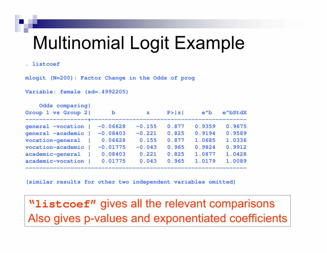
Multinomial Logit Example. listcoef
mlogit (N=200): Factor Change in the Odds of prog
Variable: female (sd=.4992205)
Odds comparing|Group 1 vs Group 2| b z P>|z| e^b e^bStdX------------------+---------------------------------------------general -vocation | -0.06628 -0.155 0.877 0.9359 0.9675general -academic | -0.08403 -0.221 0.825 0.9194 0.9589vocation-general | 0.06628 0.155 0.877 1.0685 1.0336vocation-academic | -0.01775 -0.043 0.965 0.9824 0.9912academic-general | 0.08403 0.221 0.825 1.0877 1.0428academic-vocation | 0.01775 0.043 0.965 1.0179 1.0089----------------------------------------------------------------
(similar results for other two independent variables omitted)
“listcoef” gives all the relevant comparisonsAlso gives p-values and exponentiated coefficients
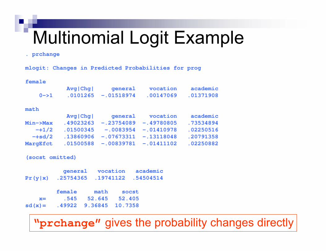
Multinomial Logit Example. prchange
mlogit: Changes in Predicted Probabilities for prog
femaleAvg|Chg| general vocation academic
0->1 .0101265 -.01518974 .00147069 .01371908
mathAvg|Chg| general vocation academic
Min->Max .49023263 -.23754089 -.49780805 .73534894-+1/2 .01500345 -.0083954 -.01410978 .02250516-+sd/2 .13860906 -.07673311 -.13118048 .20791358
MargEfct .01500588 -.00839781 -.01411102 .02250882
(socst omitted)
general vocation academicPr(y|x) .25754365 .19741122 .54504514
female math socstx= .545 52.645 52.405
sd(x)= .49922 9.36845 10.7358
“prchange” gives the probability changes directly
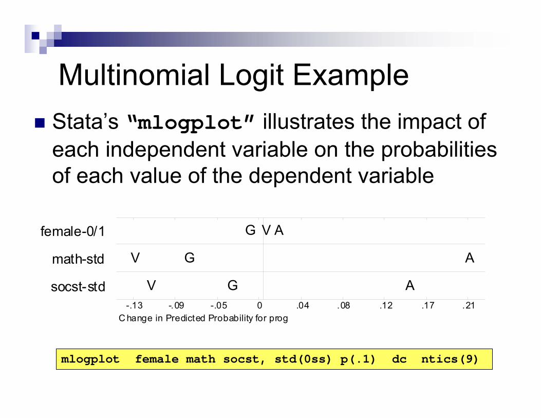
Multinomial Logit Example
mlogplot female math socst, std(0ss) p(.1) dc ntics(9)
C hange in Predicted Probability for prog -.13 -.09 -.05 0 .04 .08 .12 .17 .21
G V A
G V A
G V A
female-0/1
math-std
socst-std
Stata’s “mlogplot” illustrates the impact of each independent variable on the probabilities of each value of the dependent variable
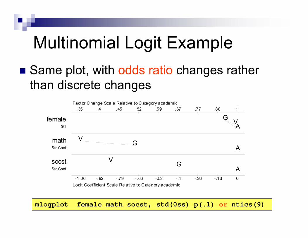
Multinomial Logit Example
mlogplot female math socst, std(0ss) p(.1) or ntics(9)
Same plot, with odds ratio changes rather than discrete changes
Factor C hange Scale Relative to C ategory academic
Logit Coefficient Scale Relative to C ategory academic
.35
-1.06
.4
-.92
.45
-.79
.52
-.66
.59
-.53
.67
-.4
.77
-.26
.88
-.13
1
0
G V A
G V
A
G V A
female 0/1
math Std Coef
socst Std Coef
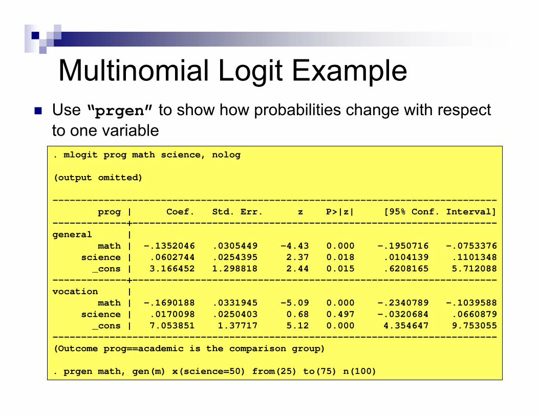
Multinomial Logit Example
. mlogit prog math science, nolog
(output omitted)
------------------------------------------------------------------------------prog | Coef. Std. Err. z P>|z| [95% Conf. Interval]
-------------+----------------------------------------------------------------general |
math | -.1352046 .0305449 -4.43 0.000 -.1950716 -.0753376science | .0602744 .0254395 2.37 0.018 .0104139 .1101348_cons | 3.166452 1.298818 2.44 0.015 .6208165 5.712088
-------------+----------------------------------------------------------------vocation |
math | -.1690188 .0331945 -5.09 0.000 -.2340789 -.1039588science | .0170098 .0250403 0.68 0.497 -.0320684 .0660879_cons | 7.053851 1.37717 5.12 0.000 4.354647 9.753055
------------------------------------------------------------------------------(Outcome prog==academic is the comparison group)
. prgen math, gen(m) x(science=50) from(25) to(75) n(100)
Use “prgen” to show how probabilities change with respect to one variable
0.2
.4.6
.81
Pro
babi
litie
s
20 40 60 80Changing value of math
pr(general) [1] pr(academic) [2] pr(vocation) [3]
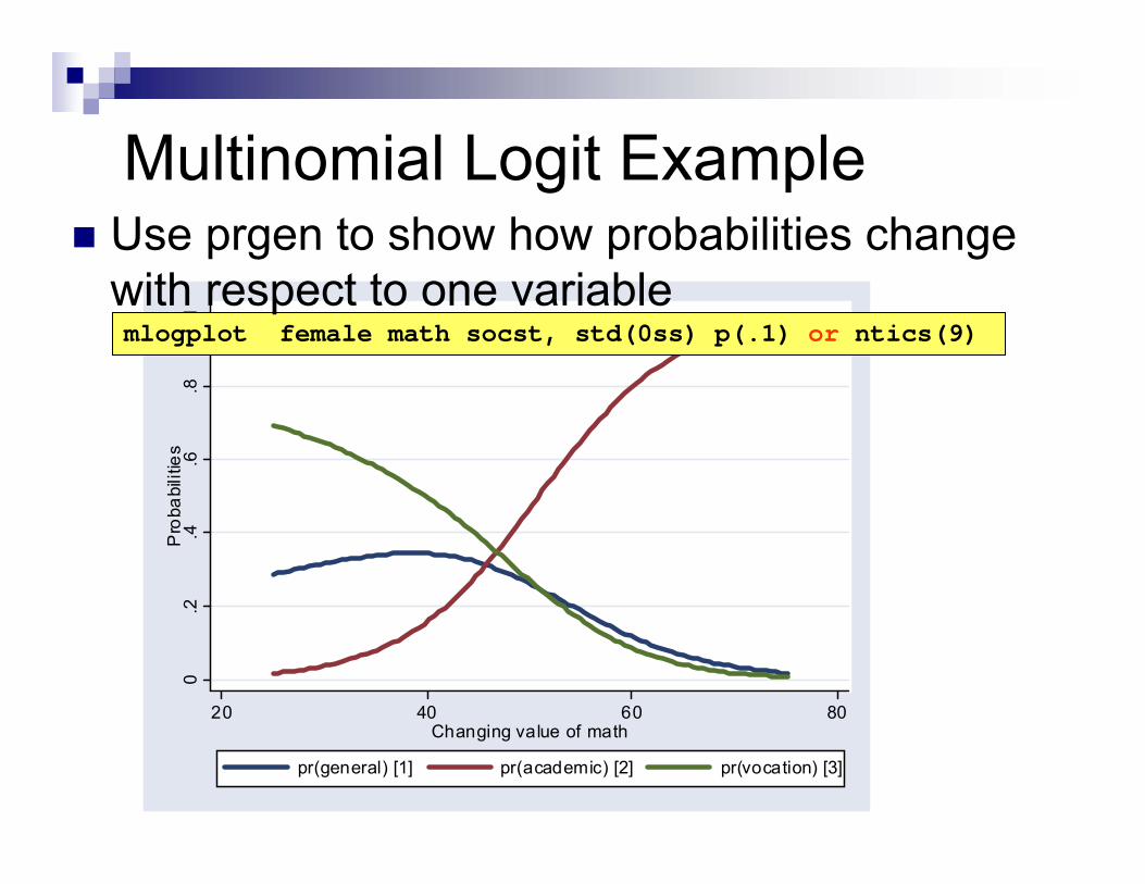
Multinomial Logit Example
mlogplot female math socst, std(0ss) p(.1) or ntics(9)
Use prgen to show how probabilities change with respect to one variable