Lecture 1: Foundations of Neoclassical Growth Acemoglu 2009, … · In macroeconomics, it is...

Lecture 1: Foundations of Neoclassical Growth(Acemoglu 2009, Chapter 5)

Adapted from Fabrizio Zilibotti’s notes

Kjetil Storesletten

August 24, 2018

Kjetil Storesletten () Lecture 1 August 24, 2018 1 / 53

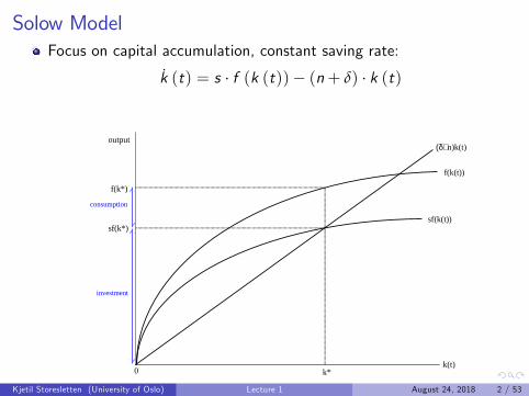
Solow ModelFocus on capital accumulation, constant saving rate:

k (t) = s · f (k (t))− (n+ δ) · k (t)

output

k(t)

f(k*)

k*

f(k(t))

sf(k*)sf(k(t))

consumption

investment

0

(δ+n)k(t)

Figure: Investment and consumption in the steady-state equilibrium withpopulation growth.

Kjetil Storesletten (University of Oslo) Lecture 1 August 24, 2018 2 / 53

Foundations of Neoclassical Growth

More satisfactory to specify the preference orderings ofindividuals and derive their decisions from these preferences

Enables better understanding of the factorsaffecting savings decisions

Enables to discuss the “optimality”of equilibria

Allows researchers to ask whether the decentralized equilibriaof growth models can be “improved upon”

Notion of improvement: Pareto optimality


Preliminaries I

Consider an economy consisting of a unit measureof infinitely-lived households

E.g., the set of households H could be representedby the unit interval [0, 1]

This representation as a continuum emphasizes that eachhousehold is infinitesimal and has no effect on aggregates

Can alternatively think of H as a countable set of the formH = {1, 2, ...,M} with M → ∞, without any loss of generalityAdvantage of unit measure: averages and aggregates are the same


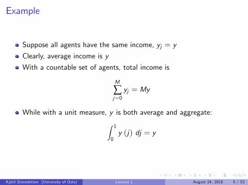
Example

Suppose all agents have the same income, yj = y

Clearly, average income is y

With a countable set of agents, total income is

M

∑j=0yj = My

While with a unit measure, y is both average and aggregate:∫ 1

0y (j) dj = y


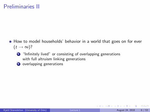
Preliminaries II

How to model households’behavior in a world that goes on for ever(t → ∞)?

1 “Infinitely lived”or consisting of overlapping generationswith full altruism linking generations

2 overlapping generations


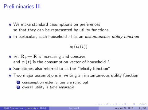
Preliminaries III

We make standard assumptions on preferencesso that they can be represented by utility functions

In particular, each household i has an instantaneous utility function

ui (ci (t))

ui : R+→ R is increasing and concaveand ci (t) is the consumption vector of household i .

Sometimes also referred to as the “felicity function”

Two major assumptions in writing an instantaneous utility function1 consumption externalities are ruled out2 overall utility is time separable


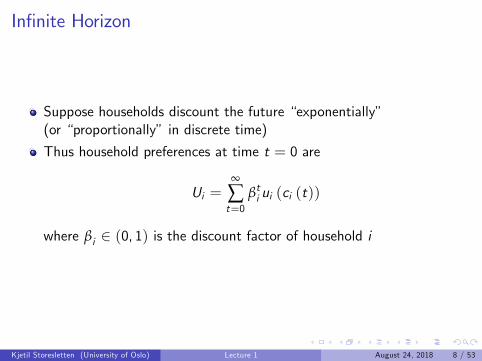
Infinite Horizon

Suppose households discount the future “exponentially”(or “proportionally” in discrete time)

Thus household preferences at time t = 0 are

Ui =∞

∑t=0

βti ui (ci (t))

where βi ∈ (0, 1) is the discount factor of household i


Time Consistency

Time separability and exponential discountingensure “time-consistent”behavior.

A solution {x (t)}Tt=0 (possibly with T = ∞) is time consistent if:

I whenever {x (t)}Tt=0 is an optimal solution starting at time t = 0,

then

{x (t)}Tt=t ′ is an optimal solution to the continuationdynamic optimization problem starting from time t = t ′ ∈ [0,T ].


Uncertainty

So far, we have ignored uncertainty:the sequence {ci (t)}∞

t=0 is known with certainty.

With uncertainty, preferences of household i at time t = 0can be represented by the following (von Neumann-Morgenstern)expected utility function:

Ei0

∞

∑t=0

βti ui (ci (t))

Ei0 is the expectation operator with respect to the

information set available to household i at time t = 0.


Heterogeneity

So far we indexed individual utility function, ui (·),and the discount factor, βi , by “i”

Households could also differ according to their income processes.E.g., effective labor endowments of {ei (t)}∞

t=0,labor income of {ei (t)w (t)}∞

t=0

But at this level of generality, the problem is not tractable

In macroeconomics, it is standard to assume theexistence of a representative household.


The Representative Household I

An economy admits a representative householdif the preference (demand) side can be representedas if a single household made the aggregate consumptionand saving decisions subject to a single budget constraint

This description of a representative household is purely positive

There is a stronger notion of “normative” representative household:if we can use the utility function of the representative householdfor welfare comparisons

Simplest case that will lead to the existence of a representativehousehold: suppose each household is identical


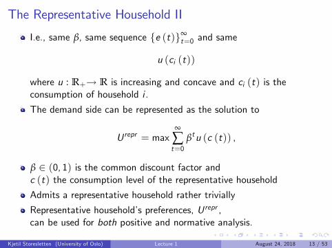
The Representative Household II

I.e., same β, same sequence {e (t)}∞t=0 and same

u (ci (t))

where u : R+→ R is increasing and concave and ci (t) is theconsumption of household i .

The demand side can be represented as the solution to

U repr = max∞

∑t=0

βtu (c (t)) ,

β ∈ (0, 1) is the common discount factor andc (t) the consumption level of the representative household

Admits a representative household rather trivially

Representative household’s preferences, U repr ,can be used for both positive and normative analysis.


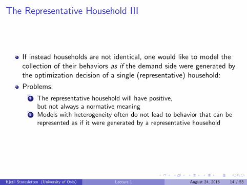
The Representative Household III

If instead households are not identical, one would like to model thecollection of their behaviors as if the demand side were generated bythe optimization decision of a single (representative) household:

Problems:1 The representative household will have positive,but not always a normative meaning

2 Models with heterogeneity often do not lead to behavior that can berepresented as if it were generated by a representative household


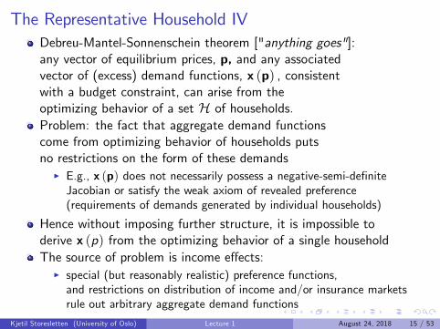
The Representative Household IVDebreu-Mantel-Sonnenschein theorem ["anything goes"]:any vector of equilibrium prices, p, and any associatedvector of (excess) demand functions, x (p) , consistentwith a budget constraint, can arise from theoptimizing behavior of a set H of households.Problem: the fact that aggregate demand functionscome from optimizing behavior of households putsno restrictions on the form of these demands

I E.g., x (p) does not necessarily possess a negative-semi-definiteJacobian or satisfy the weak axiom of revealed preference(requirements of demands generated by individual households)

Hence without imposing further structure, it is impossible toderive x (p) from the optimizing behavior of a single householdThe source of problem is income effects:

I special (but reasonably realistic) preference functions,and restrictions on distribution of income and/or insurance marketsrule out arbitrary aggregate demand functions


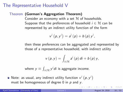
The Representative Household V

Theorem (Gorman’s Aggregation Theorem)Consider an economy with a set H of households.Suppose that the preferences of household i ∈ H can berepresented by an indirect utility function of the form

v i(p, y i

)= ai (p) + b (p) y i ,

then these preferences can be aggregated and represented bythose of a representative household, with indirect utility

v (p, y) =∫i∈H

ai (p) di + b (p) y ,

where y ≡∫i∈H y

idi is aggregate income.

Note: as usual, any indirect utility function v i(p, y i

)must be homogeneous of degree 0 in p and y .


The Representative Household VI

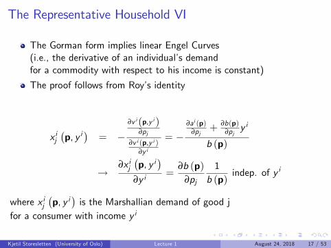
The Gorman form implies linear Engel Curves(i.e., the derivative of an individual’s demandfor a commodity with respect to his income is constant)

The proof follows from Roy’s identity

x ij(p, y i

)= −

∂v i(p,y i)∂pj

∂v i (p,y i )∂y i

= −∂ai (p)

∂pj+ ∂b(p)

∂pjy i

b (p)

→∂x ij(p, y i

)∂y i

=∂b (p)

∂pj

1b (p)

indep. of y i

where x ij(p, y i

)is the Marshallian demand of good j

for a consumer with income y i


The Representative Household VII

Quasi-linear structure limits the extent of income effectsand enables the aggregation of individual behavior

Note that (under no uncertainty) all we require is the existenceof a monotonic transformation of the indirect utility functionthat takes the Gorman form

Contains some commonly-used preferences in macroeconomics


Example: CES Preferences I

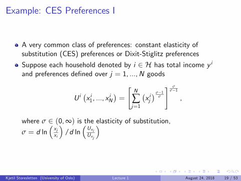
A very common class of preferences: constant elasticity ofsubstitution (CES) preferences or Dixit-Stiglitz preferences

Suppose each household denoted by i ∈ H has total income y i

and preferences defined over j = 1, ...,N goods

U i(x i1, ..., x

iN

)=

[N

∑j=1

(x ij) σ−1

σ

] σσ−1

,

where σ ∈ (0,∞) is the elasticity of substitution,σ = d ln

(xjxi

)/d ln

(UxiUxj

)


Example: CES II

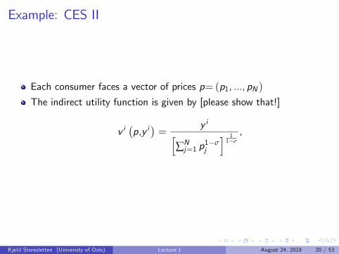
Each consumer faces a vector of prices p= (p1, ..., pN )

The indirect utility function is given by [please show that!]

v i(p,y i

)=

y i[∑Nj=1 p

1−σj

] 11−σ

,


Example: CES Preferences III

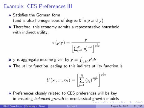
Satisfies the Gorman form(and is also homogeneous of degree 0 in p and y)

Therefore, this economy admits a representative householdwith indirect utility:

v (p,y) =y[

∑Nj=1 p

1−σj

] 11−σ

y is aggregate income given by y ≡∫i∈H y

idi

The utility function leading to this indirect utility function is

U (x1, ..., xN ) =

[N

∑j=1(xj )

σ−1σ

] σσ−1

Preferences closely related to CES preferences will be keyin ensuring balanced growth in neoclassical growth models


The Representative Household VIII

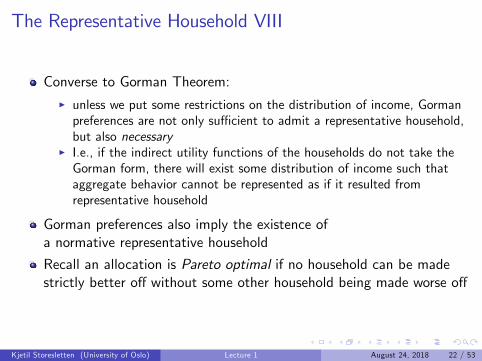
Converse to Gorman Theorem:I unless we put some restrictions on the distribution of income, Gormanpreferences are not only suffi cient to admit a representative household,but also necessary

I I.e., if the indirect utility functions of the households do not take theGorman form, there will exist some distribution of income such thataggregate behavior cannot be represented as if it resulted fromrepresentative household

Gorman preferences also imply the existence ofa normative representative household

Recall an allocation is Pareto optimal if no household can be madestrictly better off without some other household being made worse off


The Representative Household IX

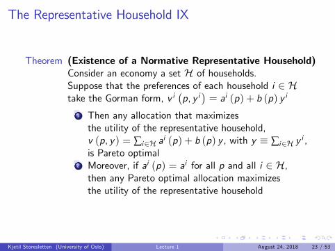
Theorem (Existence of a Normative Representative Household)Consider an economy a set H of households.Suppose that the preferences of each household i ∈ Htake the Gorman form, v i

(p, y i

)= ai (p) + b (p) y i

1 Then any allocation that maximizesthe utility of the representative household,v (p, y) = ∑i∈H a

i (p) + b (p) y , with y ≡ ∑i∈H yi ,

is Pareto optimal2 Moreover, if ai (p) = ai for all p and all i ∈ H,then any Pareto optimal allocation maximizesthe utility of the representative household


Infinite Planning Horizon I

Most growth and macro models assume that individualshave an infinite planning horizon

Two reasonable microfoundations for this assumption:1 “Poisson death model”or the perpetual youth model2 Intergenerational altruism


Poisson Death Model I

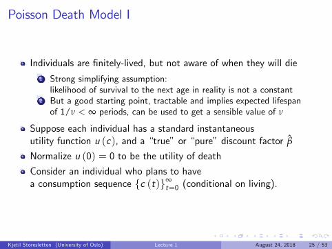
Individuals are finitely-lived, but not aware of when they will die1 Strong simplifying assumption:likelihood of survival to the next age in reality is not a constant

2 But a good starting point, tractable and implies expected lifespanof 1/ν < ∞ periods, can be used to get a sensible value of ν

Suppose each individual has a standard instantaneousutility function u (c), and a “true”or “pure”discount factor β

Normalize u (0) = 0 to be the utility of death

Consider an individual who plans to havea consumption sequence {c (t)}∞

t=0 (conditional on living).


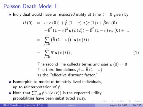
Poisson Death Model IIIndividual would have an expected utility at time t = 0 given by

U (0) = u (c (0)) + β (1− ν) u (c (1)) + βνu (0)

+β2(1− ν)2 u (c (2)) + β

2(1− ν) νu (0) + ...

=∞

∑t=0

(β (1− ν)

)tu (c (t))

=∞

∑t=0

βtu (c (t)) , (1)

The second line collects terms and uses u (0) = 0The third line defines β ≡ β (1− ν)as the “effective discount factor.”

Isomorphic to model of infinitely-lived individuals,up to reinterpretation of β.Note that ∑∞

t=0 βtu (c (t)) is the expected utility;probabilities have been substituted away.


Intergenerational Altruism I

Imagine an individual who lives for one periodand has a single offspring (who will also live for a single periodand has a single offspring etc.)

Individuals not only derives utility from consumptionbut also from the bequest they leave to their offspring


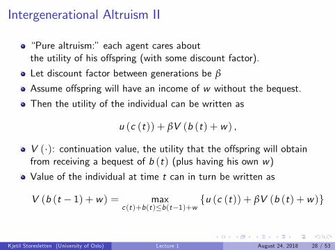
Intergenerational Altruism II

“Pure altruism:” each agent cares aboutthe utility of his offspring (with some discount factor).

Let discount factor between generations be β

Assume offspring will have an income of w without the bequest.

Then the utility of the individual can be written as

u (c (t)) + βV (b (t) + w) ,

V (·): continuation value, the utility that the offspring will obtainfrom receiving a bequest of b (t) (plus having his own w)

Value of the individual at time t can in turn be written as

V (b (t − 1) + w) = maxc (t)+b(t)≤b(t−1)+w

{u (c (t)) + βV (b (t) + w)}


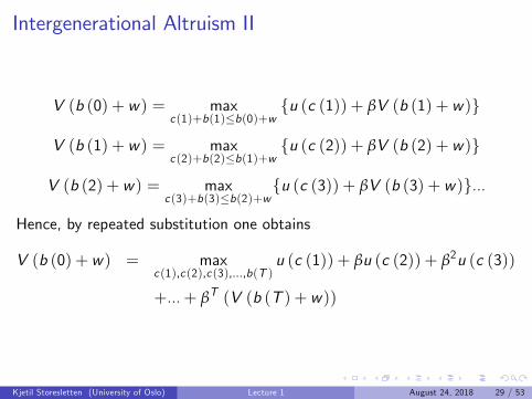
Intergenerational Altruism II

V (b (0) + w) = maxc (1)+b(1)≤b(0)+w

{u (c (1)) + βV (b (1) + w)}

V (b (1) + w) = maxc (2)+b(2)≤b(1)+w

{u (c (2)) + βV (b (2) + w)}

V (b (2) + w) = maxc (3)+b(3)≤b(2)+w

{u (c (3)) + βV (b (3) + w)}...

Hence, by repeated substitution one obtains

V (b (0) + w) = maxc (1),c (2),c (3),...,b(T )

u (c (1)) + βu (c (2)) + β2u (c (3))

+...+ βT (V (b (T ) + w))


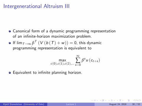
Intergenerational Altruism III

Canonical form of a dynamic programming representationof an infinite-horizon maximization problem.

If limT→∞ βT (V (b (T ) + w)) = 0, this dynamicprogramming representation is equivalent to

maxc (0),c (1),c (2),...

∞

∑s=0

βsu (ct+s )

Equivalent to infinite planning horizon.


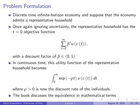
Problem Formulation

Discrete time infinite-horizon economy and suppose that the economyadmits a representative household

Once again ignoring uncertainty, the representative household has thet = 0 objective function

∞

∑t=0

βtu (c (t)) ,

with a discount factor of β ∈ (0, 1)In continuous time, this utility function of the representativehousehold becomes ∫ ∞

0exp (−ρt) u (c (t)) dt

where ρ > 0 is now the discount rate of the individuals.

The book discusses the equivalence in mathematical terms


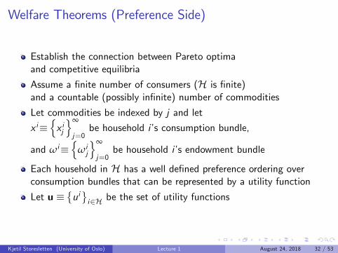
Welfare Theorems (Preference Side)

Establish the connection between Pareto optimaand competitive equilibria

Assume a finite number of consumers (H is finite)and a countable (possibly infinite) number of commodities

Let commodities be indexed by j and let

x i≡{x ij}∞

j=0be household i’s consumption bundle,

and ωi≡{

ωij

}∞

j=0be household i’s endowment bundle

Each household in H has a well defined preference ordering overconsumption bundles that can be represented by a utility function

Let u ≡{ui}i∈H be the set of utility functions


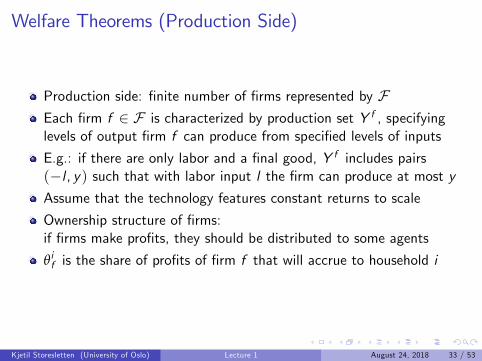
Welfare Theorems (Production Side)

Production side: finite number of firms represented by FEach firm f ∈ F is characterized by production set Y f , specifyinglevels of output firm f can produce from specified levels of inputs

E.g.: if there are only labor and a final good, Y f includes pairs(−l , y) such that with labor input l the firm can produce at most y

Assume that the technology features constant returns to scale

Ownership structure of firms:if firms make profits, they should be distributed to some agents

θif is the share of profits of firm f that will accrue to household i


Welfare Theorems (Allocation)

An economy E is described by E ≡ (H,F ,u,ω,Y,X, θ),where X denotes the choice set and Y the aggregate production set.An allocation is (x, y) such that x and y are feasible, that is,x ∈ X, y ∈ Y, and ∑i∈H x

ij ≤ ∑i∈H ωi

j +∑f ∈F yfj for all j ∈N

A price system is a sequence p≡{pj}∞j=0, such that pj ≥ 0 for all j

We can set one of these prices to unity (choice of numeraire)

We define the inner product p · x ≡ ∑∞j=0 pjxj


Welfare Theorems (Competitive Equilibrium)

Definition A competitive equilibrium for the economyE ≡ (H,F ,u,ω,Y,X, θ) is given by an allocation(x∗ =

{x i∗}i∈H , y

∗ ={y f ∗}f ∈F

)and a price system p∗

such that

1 The allocation (x∗, y∗) is feasible, i.e., x i∗ ∈ X i for alli ∈ H, y f ∗ ∈ Y f for all f ∈ F and

∑i∈H

x i∗j ≤ ∑i∈H

ωij + ∑

f ∈Fy f ∗j for all j ∈N.

2 For every firm f ∈ F , y f ∗ maximizes profits3 For every consumer i ∈ H, x i∗ maximizes utility4 All markets clear: ∑i∈H x

i∗j = ∑i∈H ωi

j +∑f ∈F yf ∗j for

all j ∈N.


Welfare Theorems (Pareto Optimality)

Definition A feasible allocation (x, y) for economyE ≡ (H,F ,u,ω,Y,X, θ) is Pareto optimalif there exists no other feasible allocation (x, y) such that

ui(x i)≥ ui

(x i)for all i ∈ H

with at least one strict inequality


First Welfare Theorem

Local nonsatiation of consumer preferences: for any bundle of goodsthere is always another bundle of goods arbitrarily close that ispreferred to it.

Formally, ∀x ∈ X and ∀ε > 0, ∃x′∈ X s.t. ‖x′ − x‖ ≤ ε and x′ ispreferred to x. If there are no "bads", it is equivalent to monotonicity.

Definition Household i ∈ H is locally non-satiated if at each x i ,ui(x i)

is strictly increasing in at least one of its arguments at x i

Theorem (First Welfare Theorem I)Suppose that (x∗, y∗, p∗) is a competitive equilibrium.Assume that all households are locally non-satiated.Then (x∗, y∗) is Pareto optimal


Second Welfare Theorem (Preliminaries) I

Converse of the First Welfare Theorem: Any Pareto optimumallocation can be decentralized as a competitive equilibrium

But requires assumptions such as the convexity of consumptionand production sets and preferences and additional requirements

Contains an “existence of equilibrium argument,”whichruns into problems in the presence of non-convexities

Under convex preferences and technology,it is easy to prove the Second Welfare Theoremwhen the number of commodity is finite

The extension to ∞ commodities is more complexbut also important for us. It requires a finite set ofcommodities to be "salient" in preferences and technology


Second Welfare Theorem (Preliminaries) II

Recall that the consumption set of each individual i ∈ H is X i

A typical element of X i is x i =(x i1, x

i2, ...

), where x it can be

interpreted as the vector of consumption of individual i at time t

Similarly, a typical element of the production setof firm f ∈ F , Y f , is y f =

(y f1 , y

f2 , ...

)Let us define the "truncations"x i [T ] =

(x i0, x

i1, x

i2, ..., x

iT , 0, 0, ...

),

y f [T ] =(y f0 , y

f1 , y

f2 , ..., y

fT , 0, 0, ...

)


Second Welfare Theorem I

Consider a Pareto optimal allocation (x∗∗, y∗∗)in an economy described by ω,

{Y f}f ∈F ,

{X i}i∈H, and

{ui (·)

}i∈H.

Suppose all production and consumption sets are convex,and all agents have continuous, convex preferencessatisfying local non-satiation

Suppose also 0 ∈ X i for each i ∈ H

Suppose ∃ T such that for any x , x ′ ∈ X i with ui (x) > ui (x ′),ui (x [T ]) > ui (x ′ [T ]) for all T ≥ T and for all i ∈ H,and that ∃ T such that if y ∈ Y f ,then y [T ] ∈ Y f for all T ≥ T and for all f ∈ F .


Second Welfare Theorem II

Then there exist p∗∗ and (ω∗∗, θ∗∗) such that in economyE ≡ (H,F ,u,ω∗∗,Y,X, θ∗∗),

1 ω∗∗ satisfies ω = ∑i∈H ωi∗∗;2 (profits are maximized) for all f ∈ F ,

p∗∗ · y f ∗∗ ≥ p∗∗ · y for all y ∈ Y f ;

3 (utilities are maximized) for all i ∈ H,

if x i ∈ X i involves ui(x i)> ui

(x i∗∗

), then p∗∗ · x i ≥ p∗∗ · w i∗∗,

where w i∗∗ ≡ ωi∗∗ +∑f ∈F θi∗∗f y f ∗∗.

Moreover, if p∗∗ ·w∗∗ > 0 [i.e., p∗∗ · w i∗∗ > 0 for each i ∈ H],then economy E has a competitive equilibrium (x∗∗, y∗∗,p∗∗).


Second Welfare Theorem (Comments) I

Remark 1:I If we have a finite commodity space, say with K commodities, then thehypothesis that there exists T with the properties defined above wouldbe satisfied automatically, by taking T = T = K .

I In dynamic economies, its role is changes in allocations at very far inthe future should not have a large effect.

Remark 2:I The conditions are stronger than for the First W.Th.i.e., stronger conditions are required for anyPareto optimal allocation to be decentralizable

I The decentralization of a Pareto optimumis subject in general to reallocation of endowments.In reality this may be diffi cult (or costly) to achieve


Second Welfare Theorem (Comments) II

Under the conditions of the SWT a competitive equilibrium must exist

The SWT motivates many macroeconomists to look for the set ofPareto optimal allocations instead of explicitly characterizingcompetitive equilibria

Real power of the Theorem in dynamic macro models comes when wecombine it with models that admit a representative household

Enables us to characterize the optimal growth allocation thatmaximizes the utility of the representative household and assert thatthis will correspond to a competitive equilibrium


Sequential Trading and Arrow-Debreu Equilibrium

GE models assume that all commodities are tradedat a given point in time– once and for all.

Arrow-Debreu Equilibrium (AD):all households trade at t = 0 and purchase or sell irrevocableclaims to commodities indexed by date and state of nature.

In models of economic growth, it is realistic to modeltrade as taking place at different points in time

Sequential Trade Equilibrium (ST):separate markets open at each t, and households trade labor,capital and consumption goods in each such market.

With complete markets and time-consistent preferences,AD equilibrium and ST equilibrium are equivalent.


A Simple Example

Consider a simple dynamic exchange economy, t ∈ {0, 1}.There are 2 goods at each date, j ∈ {A,B}.Denote the consumption of good j by household i at time t as x ij ,t .

Goods are perishable, so that they are indeed consumed at time t.

Each household i ∈ H has a vector of endowment(ωiA,t ,ω

iB ,t

)at time t, and (time-consistent) preferences

U =1

∑t=0

βti ui (x iA,t , x iB ,t) .


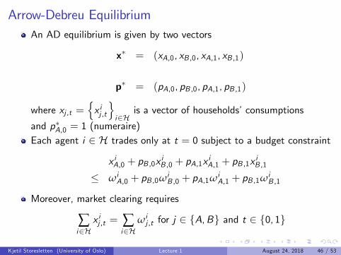
Arrow-Debreu EquilibriumAn AD equilibrium is given by two vectors

x∗ = (xA,0, xB ,0, xA,1, xB ,1)

p∗ = (pA,0, pB ,0, pA,1, pB ,1)

where xj ,t ={x ij ,t}i∈H

is a vector of households’consumptions

and p∗A,0 = 1 (numeraire)Each agent i ∈ H trades only at t = 0 subject to a budget constraint

x iA,0 + pB ,0xiB ,0 + pA,1x

iA,1 + pB ,1x

iB ,1

≤ ωiA,0 + pB ,0ω

iB ,0 + pA,1ω

iA,1 + pB ,1ω

iB ,1

Moreover, market clearing requires

∑i∈H

x ij ,t = ∑i∈H

ωij ,t for j ∈ {A,B} and t ∈ {0, 1}


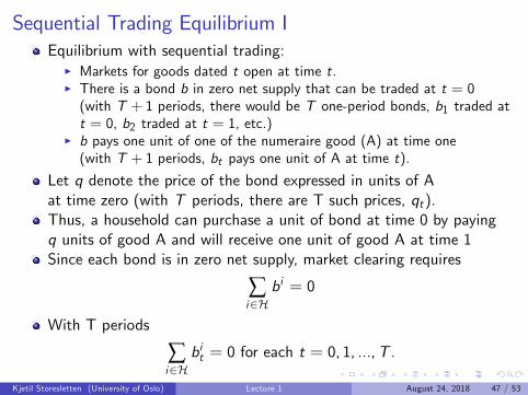
Sequential Trading Equilibrium IEquilibrium with sequential trading:

I Markets for goods dated t open at time t.I There is a bond b in zero net supply that can be traded at t = 0(with T + 1 periods, there would be T one-period bonds, b1 traded att = 0, b2 traded at t = 1, etc.)

I b pays one unit of one of the numeraire good (A) at time one(with T + 1 periods, bt pays one unit of A at time t).

Let q denote the price of the bond expressed in units of Aat time zero (with T periods, there are T such prices, qt).Thus, a household can purchase a unit of bond at time 0 by payingq units of good A and will receive one unit of good A at time 1Since each bond is in zero net supply, market clearing requires

∑i∈H

bi = 0

With T periods

∑i∈H

bit = 0 for each t = 0, 1, ...,T .


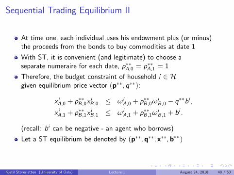
Sequential Trading Equilibrium II

At time one, each individual uses his endowment plus (or minus)the proceeds from the bonds to buy commodities at date 1

With ST, it is convenient (and legitimate) to choose aseparate numeraire for each date, p∗∗A,0 = p

∗∗A,1 = 1

Therefore, the budget constraint of household i ∈ Hgiven equilibrium price vector (p∗∗, q∗∗):

x iA,0 + p∗∗B ,0x

iB ,0 ≤ ωi

A,0 + p∗∗B ,0ω

iB ,0 − q∗∗bi ,

x iA,1 + p∗∗B ,1x

iB ,1 ≤ ωi

A,1 + p∗∗B ,1ω

iB ,1 + b

i .

(recall: bi can be negative - an agent who borrows)

Let a ST equilibrium be denoted by (p∗∗,q∗∗, x∗∗,b∗∗)


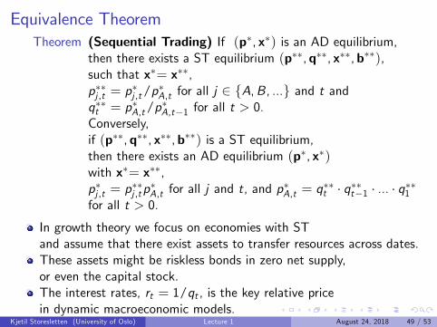
Equivalence TheoremTheorem (Sequential Trading) If (p∗, x∗) is an AD equilibrium,

then there exists a ST equilibrium (p∗∗,q∗∗, x∗∗,b∗∗),such that x∗= x∗∗,p∗∗j ,t = p

∗j ,t/p

∗A,t for all j ∈ {A,B, ...} and t and

q∗∗t = p∗A,t/p∗A,t−1 for all t > 0.

Conversely,if (p∗∗,q∗∗, x∗∗,b∗∗) is a ST equilibrium,then there exists an AD equilibrium (p∗, x∗)with x∗= x∗∗,p∗j ,t = p

∗∗j ,tp∗A,t for all j and t, and p

∗A,t = q

∗∗t · q∗∗t−1 · ... · q∗∗1

for all t > 0.

In growth theory we focus on economies with STand assume that there exist assets to transfer resources across dates.These assets might be riskless bonds in zero net supply,or even the capital stock.The interest rates, rt = 1/qt , is the key relative pricein dynamic macroeconomic models.


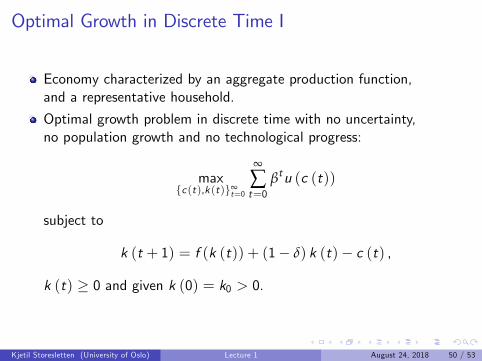
Optimal Growth in Discrete Time I

Economy characterized by an aggregate production function,and a representative household.

Optimal growth problem in discrete time with no uncertainty,no population growth and no technological progress:

max{c (t),k (t)}∞

t=0

∞

∑t=0

βtu (c (t))

subject to

k (t + 1) = f (k (t)) + (1− δ) k (t)− c (t) ,

k (t) ≥ 0 and given k (0) = k0 > 0.


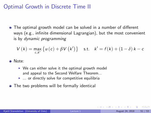
Optimal Growth in Discrete Time II

The optimal growth model can be solved in a number of differentways (e.g., infinite dimensional Lagrangian), but the most convenientis by dynamic programming

V (k) = maxc ,k ′

{u (c) + βV

(k ′)}

s.t. k ′ = f (k) + (1− δ) k − c

Note:I We can either solve it the optimal growth modeland appeal to the Second Welfare Theorem...

I ... or directly solve for competitive equilibria

The two problems will be formally identical


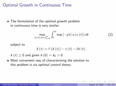
Optimal Growth in Continuous Time

The formulation of the optimal growth problemin continuous time is very similar:

max[c (t),k (t)]∞t=0

∫ ∞

0exp (−ρt) u (c (t)) dt (2)

subject tok (t) = f (k (t))− c (t)− δk (t) ,

k (t) ≥ 0 and given k (0) = k0 > 0.Most convenient way of characterizing the solution tothis problem is via optimal control theory.


Conclusions

The models we study in this course are examplesof more general dynamic general equilibrium models.

First and the Second Welfare Theorems are essential.

The most general class of dynamic general equilibrium models are nottractable enough to derive sharp results about economic growth.

Need simplifying assumptions, the most important one beingthe representative household assumption.

Sequential trade is the natural assumption in dynamic economies.However, we can exploit equivalence results with Arrow-Debreuequilibrium and invoke standard results in GE theory.


Lecture 1: Foundations of Neoclassical Growth Acemoglu 2009, … · In macroeconomics, it is...

Documents

Transcript of Lecture 1: Foundations of Neoclassical Growth Acemoglu 2009, … · In macroeconomics, it is...