Learning Discriminative αβ-Divergences for Positive Definite Matrices

1A. Cherian∗ 2P. Stanitsas∗ 3M. Harandi 2V. Morellas 2N. Papanikolopoulos1Australian Centre for Robotic Vision, 3Data61/CSIRO, 1,3The Australian National University

2Dept. of Computer Science, University of Minnesota, Minneapolis

{anoop.cherian, mehrtash.harandi}@anu.edu.au, {stani078, morellas, npapas}@umn.edu

Abstract

Symmetric positive definite (SPD) matrices are useful for

capturing second-order statistics of visual data. To com-

pare two SPD matrices, several measures are available,

such as the affine-invariant Riemannian metric, Jeffreys di-

vergence, Jensen-Bregman logdet divergence, etc.; how-

ever, their behaviors may be application dependent, rais-

ing the need of manual selection to achieve the best pos-

sible performance. Further and as a result of their over-

whelming complexity for large-scale problems, computing

pairwise similarities by clever embedding of SPD matri-

ces is often preferred to direct use of the aforementioned

measures. In this paper, we propose a discriminative met-

ric learning framework, Information Divergence and Dic-

tionary Learning (IDDL), that not only learns application

specific measures on SPD matrices automatically, but also

embeds them as vectors using a learned dictionary. To learn

the similarity measures (which could potentially be distinct

for every dictionary atom), we use the recently introduced

αβ-logdet divergence, which is known to unify the mea-

sures listed above. We propose a novel IDDL objective, that

learns the parameters of the divergence and the dictionary

atoms jointly in a discriminative setup and is solved effi-

ciently using Riemannian optimization. We showcase exten-

sive experiments on eight computer vision datasets, demon-

strating state-of-the-art performances.

1. Introduction

Symmetric Positive Definite (SPD) matrices arise natu-

rally in several computer vision applications, such as co-

variances when modeling data using Gaussians, as kernel

matrices for high-dimensional embedding, as points in dif-

fusion MRI [37], and as structure tensors in image process-

ing [5]. Furthermore, SPD matrices in the form of Region

CoVariance Descriptors (RCoVDs) [44], offer an easy way

to compute a representation that fuses multiple modalities

∗Equal contribution.

X

Bi X

Bk

Bj

X

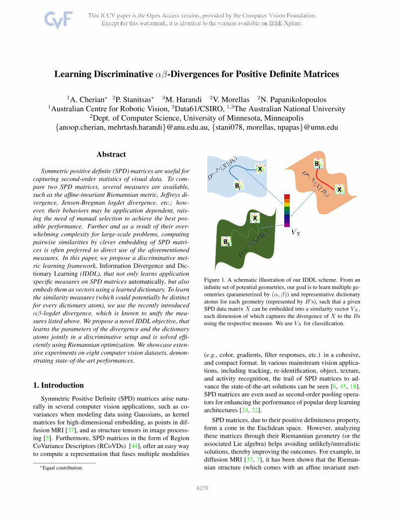
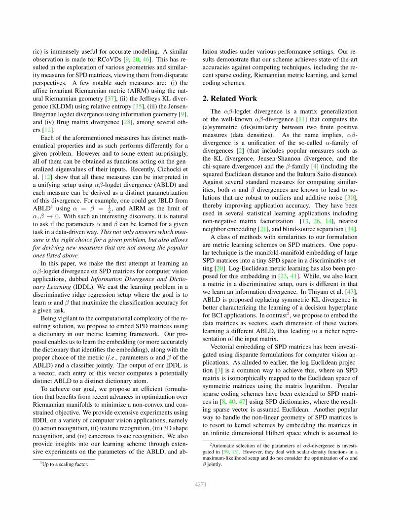
Figure 1. A schematic illustration of our IDDL scheme. From an

infinite set of potential geometries, our goal is to learn multiple ge-

ometries (parameterized by (α, β)) and representative dictionary

atoms for each geometry (represented by B’s), such that a given

SPD data matrix X can be embedded into a similarity vector VX ,

each dimension of which captures the divergence of X to the Bs

using the respective measure. We use VX for classification.

(e.g., color, gradients, filter responses, etc.) in a cohesive,

and compact format. In various mainstream vision applica-

tions, including tracking, re-identification, object, texture,

and activity recognition, the trail of SPD matrices to ad-

vance the state-of-the-art solutions can be seen [6, 45, 18].

SPD matrices are even used as second-order pooling opera-

tors for enhancing the performance of popular deep learning

architectures [24, 22].

SPD matrices, due to their positive definiteness property,

form a cone in the Euclidean space. However, analyzing

these matrices through their Riemannian geometry (or the

associated Lie algebra) helps avoiding unlikely/unrealistic

solutions, thereby improving the outcomes. For example, in

diffusion MRI [37, 3], it has been shown that the Rieman-

nian structure (which comes with an affine invariant met-

14270

ric) is immensely useful for accurate modeling. A similar

observation is made for RCoVDs [9, 20, 46]. This has re-

sulted in the exploration of various geometries and similar-

ity measures for SPD matrices, viewing them from disparate

perspectives. A few notable such measures are: (i) the

affine invariant Riemannian metric (AIRM) using the nat-

ural Riemannian geometry [37], (ii) the Jeffreys KL diver-

gence (KLDM) using relative entropy [35], (iii) the Jensen-

Bregman logdet divergence using information geometry [9],

and (iv) Brug matrix divergence [28], among several oth-

ers [12].

Each of the aforementioned measures has distinct math-

ematical properties and as such performs differently for a

given problem. However and to some extent surprisingly,

all of them can be obtained as functions acting on the gen-

eralized eigenvalues of their inputs. Recently, Cichocki et

al. [12] show that all these measures can be interpreted in

a unifying setup using αβ-logdet divergence (ABLD) and

each measure can be derived as a distinct parametrization

of this divergence. For example, one could get JBLD from

ABLD1 using α = β = 12 , and AIRM as the limit of

α, β → 0. With such an interesting discovery, it is natural

to ask if the parameters α and β can be learned for a given

task in a data-driven way. This not only answers which mea-

sure is the right choice for a given problem, but also allows

for deriving new measures that are not among the popular

ones listed above.

In this paper, we make the first attempt at learning an

αβ-logdet divergence on SPD matrices for computer vision

applications, dubbed Information Divergence and Dictio-

nary Learning (IDDL). We cast the learning problem in a

discriminative ridge regression setup where the goal is to

learn α and β that maximize the classification accuracy for

a given task.

Being vigilant to the computational complexity of the re-

sulting solution, we propose to embed SPD matrices using

a dictionary in our metric learning framework. Our pro-

posal enables us to learn the embedding (or more accurately

the dictionary that identifies the embedding), along with the

proper choice of the metric (i.e., parameters α and β of the

ABLD) and a classifier jointly. The output of our IDDL is

a vector, each entry of this vector computes a potentially

distinct ABLD to a distinct dictionary atom.

To achieve our goal, we propose an efficient formula-

tion that benefits from recent advances in optimization over

Riemannian manifolds to minimize a non-convex and con-

strained objective. We provide extensive experiments using

IDDL on a variety of computer vision applications, namely

(i) action recognition, (ii) texture recognition, (iii) 3D shape

recognition, and (iv) cancerous tissue recognition. We also

provide insights into our learning scheme through exten-

sive experiments on the parameters of the ABLD, and ab-

1Up to a scaling factor.

lation studies under various performance settings. Our re-

sults demonstrate that our scheme achieves state-of-the-art

accuracies against competing techniques, including the re-

cent sparse coding, Riemannian metric learning, and kernel

coding schemes.

2. Related Work

The αβ-logdet divergence is a matrix generalization

of the well-known αβ-divergence [11] that computes the

(a)symmetric (dis)similarity between two finite positive

measures (data densities). As the name implies, αβ-

divergence is a unification of the so-called α-family of

divergences [2] (that includes popular measures such as

the KL-divergence, Jensen-Shannon divergence, and the

chi-square divergence) and the β-family [4] (including the

squared Euclidean distance and the Itakura Saito distance).

Against several standard measures for computing similar-

ities, both α and β divergences are known to lead to so-

lutions that are robust to outliers and additive noise [30],

thereby improving application accuracy. They have been

used in several statistical learning applications including

non-negative matrix factorization [13, 26, 14], nearest

neighbor embedding [21], and blind-source separation [34].

A class of methods with similarities to our formulation

are metric learning schemes on SPD matrices. One popu-

lar technique is the manifold-manifold embedding of large

SPD matrices into a tiny SPD space in a discriminative set-

ting [20]. Log-Euclidean metric learning has also been pro-

posed for this embedding in [23, 41]. While, we also learn

a metric in a discriminative setup, ours is different in that

we learn an information divergence. In Thiyam et al. [43],

ABLD is proposed replacing symmetric KL divergence in

better characterizing the learning of a decision hyperplane

for BCI applications. In contrast2, we propose to embed the

data matrices as vectors, each dimension of these vectors

learning a different ABLD, thus leading to a richer repre-

sentation of the input matrix.

Vectorial embedding of SPD matrices has been investi-

gated using disparate formulations for computer vision ap-

plications. As alluded to earlier, the log-Euclidean projec-

tion [3] is a common way to achieve this, where an SPD

matrix is isomorphically mapped to the Euclidean space of

symmetric matrices using the matrix logarithm. Popular

sparse coding schemes have been extended to SPD matri-

ces in [8, 40, 47] using SPD dictionaries, where the result-

ing sparse vector is assumed Euclidean. Another popular

way to handle the non-linear geometry of SPD matrices is

to resort to kernel schemes by embedding the matrices in

an infinite dimensional Hilbert space which is assumed to

2Automatic selection of the parameters of αβ-divergence is investi-

gated in [39, 15]. However, they deal with scalar density functions in a

maximum-likelihood setup and do not consider the optimization of α and

β jointly.

4271

be linear [19, 32, 18]. In all these methods, the underly-

ing similarity measure is fixed and is usually chosen to be

one among the popular αβ-logdet divergences or the log-

Euclidean metric.

In contrast to all these methods, to the best of our knowl-

edge, it is for the first time that a joint dictionary learning

and information divergence learning framework is proposed

for SPD matrices in computer vision. In the sequel, we first

introduce αβ-logdet divergence and explore its properties

in the next section. This will precede exposition to our dis-

criminative metric learning framework for learning the di-

vergence and efficient ways of solving our formulation.

Notations: Following standard notations, we use upper

case for matrices (such as X), lower-bold case for vectors

x, and lower case for scalars x. Further, Sd++ is used to de-

note the cone of d× d SPD matrices. We use B to denote a

3D tensor each slice of which is an SPD matrix of size d×d.

Further, we use Id to denote the d × d identity matrix, Logfor the matrix logarithm, and diag for the diagonalization

operator.

3. Background

In this section, we will setup the mathematical prelimi-

naries necessary to elucidate our contributions. We will visit

the αβ-log-det divergence, its connections to other popular

divergences, and its mathematical properties.

3.1. αβ­Log Determinant Divergence

Definition 1 (ABLD [12]) For X,Y ∈ Sd++, the αβ-log-

det divergence is defined as:

D(α,β)(X‖Y )=1

αβlog det

(

α(XY −1)β+β(XY −1)−α

α+ β

)

,

(1)

α 6= 0, β 6= 0 and α+ β 6= 0. (2)

It can be shown that ABLD depends only on the gener-

alized eigenvalues of X and Y [12]. Suppose λi denotes

the i-th eigenvalue of XY−1

. Then under constraints defined

in (2), we can rewrite (1) as:

D(α,β)(X‖Y)=1

αβ

d∑

i=1

log(

αλβi +βλ−α

i

)

−d log (α+β).

(3)

This formulation will come handy when deriving the gradi-

ent updates for α and β in the sequel. As alluded to earlier,

a hallmark of the ABLD is that it unifies several popular

distance measures on SPD matrices that one commonly en-

counters in computer vision applications. In Table 1, we list

some of the popular measures in computer vision and the

respective values of α and β.

3.2. ABLD Properties

Avoiding Degeneracy: An important observation regard-

ing the design of optimization algorithms on ABLD is that

the quantity inside the log det term has to be positive def-

inite; conditions on α and β for which are specified by the

following theorem.

Theorem 1 ([12]) For X,Y ∈ Sd++, if λi is the i-th eigen-

value of X−1Y , then D(α,β)(X ‖ Y ) ≥ 0 only if

λi >

∣

∣

∣

∣

α

β

∣

∣

∣

∣

1α+β

, for α > 0 and β < 0, or (4)

λi <

∣

∣

∣

∣

β

α

∣

∣

∣

∣

1α+β

, for α < 0 and β > 0, ∀i = 1, 2, · · · , d. (5)

Since λis depend on the input matrices, on which we

have no control over, we constrain α and β to have the same

sign, thereby avoiding the quantity inside log det to be in-

definite. We make this assumption in our formulations in

Section 4.

Smoothness of α, β: Assuming α, β have the same sign,

except at origin (α = β = 0), ABLD is smooth every-

where with respect to α and β, thus allowing us to develop

Newton-type algorithms on them. Due to the discontinu-

ity at the origin, we ought to design algorithms specifically

addressing this particular case.

Affine Invariance: It can be easily shown that

D(α,β)(X ‖ Y ) = D(α,β)(AXAT ‖ AY AT ), (6)

for any invertible matrix A. This is an important property

that makes this divergence useful in a variety of applica-

tions, such as diffusion MRI [37].

Dual Symmetry: This property allows us to extend results

derived for the case of α to the one on β later.

D(α,β)(X ‖ Y ) = D(β,α)(Y ‖ X). (7)

Before concluding this part, we briefly introduce the con-

cept of optimization on Riemannian manifolds and in par-

ticular the method of Riemmanian Conjugate Gradient de-

scent (RCG).

3.3. Optimization on Riemannian Manifolds

As will be shown in § 4, we need to solve a non-convex

constrained optimization problem in the form

minimize L(B)

s.t. B ∈ Sd++ . (8)

Classical optimization methods generally turn a con-

strained problem into a sequence of unconstrained prob-

lems for which unconstrained techniques can be applied.

4272

(α, β) ABLD Divergence

(α, β)→ 0∥

∥

∥LogX−

12Y X−

12

∥

∥

∥

2

FSquared Affine Invariant Riemannian Metric [37]

α = β = ± 12 4

(

log det X+Y2 − 1

2 log detXY)

Jensen-Bregman Logdet Divergence [9]

α = ±1, β → 0 12Tr

(

XY−1+ Y X

−1)

− d Jeffreys KL Divergence3 [35]

α = 1, β = 1 Tr(

XY−1)

− log detXY−1− d Burg Matrix Divergence [28]

Table 1. ABLD and its connections to popular divergences used in computer vision applications.

In contrast, in this paper we make use of the optimization

on Riemannian manifolds to minimize (8). This is moti-

vated by recent advances in Riemannian optimization tech-

niques where benefits of exploiting geometry over standard

constrained optimization are shown [1]. As a consequence,

these techniques have become increasingly popular in di-

verse application domains [8, 18].

A detailed discussion of Riemannian optimization goes

beyond the scope of this paper, and we refer the interested

reader to [1]. However, the knowledge of some basic con-

cepts will be useful in the remainder of this paper. As such,

here, we briefly consider the case of Riemannian Conju-

gate Gradient method (RCG), our choice when the empiri-

cal study of this work is considered. First we formally de-

fine the SPD manifold.

Definition 2 (The SPD Manifold) The set of (d × d) di-

mensional real, SPD matrices endowed with the Affine In-

variant Riemannian Metric (AIRM) [37] forms the SPD

manifold Sd++.

Sp++ , {X ∈ Rd×d : vTXv > 0, ∀v ∈ R

d−{0d}} . (9)

To minimize (8), RCG starts from an initial solution B(0)

and improves its solution using the update rule

B(t+1) = τB(t)

(

P (t))

, (10)

where P (t) identifies a search direction and τB(·) :TBS

d++ → S

d++ is a retraction. The retraction serves to

identify the new solution along the geodesic defined by the

search direction P (t). In RCG, it is guaranteed that the new

solution obtained by Eq. (10) is on Sd++ and has a lower ob-

jective. The search direction P (t) ∈ TB(t)Sd++ is obtained

by

P (t) = −grad L(B(t)) + η(t)π(P (t−1), B(t−1), B(t)) .(11)

Here, η(t) can be thought of as a variable learning rate,

obtained via techniques such as Fletcher-Reeves [1]. Fur-

thermore, grad L(B) is the Riemannian gradient of the ob-

jective function at B and π(P,X, Y ) denotes the parallel

transport of P from TX to TY . In Table 2, we define the

mathematical entities required to perform RCG on the SPD

manifold. Note that computing the standard Euclidean gra-

dient of the function L, denoted by ∇∗(L), is the only re-

quirement to perform RCG on Sd++.

Sd

++

Riemannian gradient grad L(B) = Bsym(

∇B(L))

B

Retraction. τB(ξ) = B12 Exp(B−

12 ξB−

12 )B

12

Parallel Transport. π(P,X, Y ) = ZPZT

Table 2. Riemannian tools to perform RCG on Sd

++. Here,

sym(X) = 1

2(X +XT ), Exp(·) denotes the matrix exponential

and Z = (Y X−1)12 .

4. Proposed Method

In this section, we first introduce the most general form

of our joint IDDL formulation and follow it up by providing

simplifications and derivations for specific cases (such as

for α = β = 0).

4.1. Information Divergence & Dictionary Learning

Suppose we are given a set of SPD matrices X ={X1, X2, · · · , XN} , Xi ∈ S

d++ along their associated la-

bels yi ∈ L = {1, 2, · · · , L}. Our goal is three-fold: (i)

learn a dictionary B ∈ Sd++×n, a product of n SPD man-

ifolds, (ii) learn an ABLD on each dictionary atom to best

represent the given data for the task of classification, and

(iii) learn a discriminative objective function on the encoded

SPD matrices (in terms of B and the respective ABLDs) for

the purpose of classification. These goals are formally cap-

tured in the IDDL objective proposed below. Let the k-th

dictionary atom in B be Bk, then,

IDDL := minB>0,α>0,β>0,W

N∑

i=1

f(vi, yi;W ) (12)

subject to vki = D(αk,βk)(Xi ‖ Bk),

where the vector vi ∈ Rn denotes the encoding of Xi in

terms of the dictionary, and vki is the k-th dimension of

this encoding. The function f parameterized by W learns a

classifier on vi according to the provided class labels yi.

While, there are several choices for f (e.g., max-margin

hinge-loss), we resort to a simple ridge regression objec-

tive in this paper. Thus, our f is defined as follows: sup-

pose hi ∈ {0, 1}n is a one-off encoding of class labels (i.e.,

hyi

i = 1, everywhere else zero), then

f(vi, yi;W ) =1

2‖hi −Wvi‖

2+ γ ‖W‖

2F , (13)

4273

where W ∈ RL×n and γ is a regularization parameter. Note

that a separate αk, βk for each dictionary atom is the most

general form of our formulation. In our experiments, we

explore simplified cases when these parameters are shared

across the atoms.

4.2. Efficient Optimization

In this section, we propose efficient ways to solve the

IDDL objective in (12). We propose to use a block-

coordinate descent (BCD) scheme for optimization, in

which each variable is updated alternately while fixing oth-

ers. Going by the recent trends in Riemannian optimization

for SPD matrices [8, 18], we use the Riemannian conjugate

gradient (RCG) algorithm [1] for optimizing over each vari-

able. As our objective is non-convex in its variables (except

for W ), convergence of BCD iterations to a global minima

is not guaranteed. In Alg. 1, we detail out the meta-steps in

our optimization scheme. We initialize the dictionary atoms

and the divergence parameters as described in Section 6.3.

Following that, we update the atoms, the divergence pa-

rameters, and classifier parameters in an alternating man-

ner manner – that is, updating one variable whie fixing all

others.

Recall from Section 3.3 that an essential ingredient in

RCG is efficient computations of the Euclidean gradients of

the objective with respect to the variables. In the following,

we derive expressions for these gradients. Note that we as-

sume that the dictionary atoms (i.e., Bi) to be on an SPD

manifold. Also w.l.o.g, we assume α and β belong to the

non-negative orthant of the Euclidean space (for reasons in

Section 3).

Input: X , H , n

B← kmeans(X , n), (α,β)← GridSearch;

repeat

for k = 1 to n doBk ← update B(X ,W,α,β, Bk); // use (18)

end

(α,β)← update αβ(X ,W,B,α,β); // use (20)

W ← update W ; // using (21)

until until convergence;

return B,α,β

Algorithm 1: Block-Coordinate Descent for IDDL.

4.2.1 Gradients wrt B

As is clear from our formulation, only the k-th dimension

of vi involves Bk. To simplify the notations, let us assume

ζ = −(hi −Wvi)TW, (14)

and let ζk be its k-th dimension. Then we have (see the

supplementary material for the details),

∇Bkf := ζki ∇Bk

(

D(αk,βk)(Xi ‖ Bk))

. (15)

Substituting for ABLD in (15) and rearranging the terms,

we have:

∇Bkf =

1

αkβk

∇Bklog det

[

αk

βk

(

Xi−1Bk

)αk+βk + Id

]

−1

βk

Bk−1. (16)

Let θk = αk + βk and rk = αk

βk. Further, let Zi = Xi

−1.

Then, the term inside the gradient in (16) simplifies to:

g(Bk;Z, rk, θk) = log det[

rk (ZBk)θk + Id

]

. (17)

Theorem 2 Let A,B ∈ Sd++. Furthermore assume p, q ≥0. We have

∇B log det [p (AB)q+ Id]=

pqB−1A−

12

(

A12BA

12

)q(

Id + p(

A12BA

12

)q)−1

A12 .

Proof See the extended version of this paper [10].

As such, the gradient ∇Bkg is:

∇Bkg=rkθkBk

−1Z

−12

i

(

Z12i BkZ

12i

)θk

×

(

Id + rk

(

Z12i BkZ

12i

)θk)

−1

Z12i . (18)

Combining (18) with (16), we have the expression for the

gradient with respect to Bk.

Remark 1 Computing ∇Bkg for large datasets may be-

come overwhelming. Let (Ui,∆i) be the Schur decomposi-

tion Z12i BkZ

12i (which is faster than the eigenvalue decom-

position [17]). With δi = diag(∆i), the gradient in (18)

can be rewritten as:

∇Bkg = rkθkBk

−1(

Z−

12

i Ui

)

[

diag

(

δθi

1 + rkδθki

)]

×(

Z−

12

i Ui

)

−1. (19)

Compared to (18), this simplification reduces the number

of matrix multiplications from 5 to 3 and matrix inversions

from 2 to 1.

4274

4.2.2 Gradients wrt αk and βk

For gradients with respect to αk, we will use the form of

ABLD given in (3), where λijk is assumed to be the j-th

generalized eigenvalue of Xi and dictionary atom Bk. Us-

ing the notations defined in (14), the gradient has the form:

∇αkf = ζki

d∑

j=1

∇αk

[

1

αkβk

logαkλ

βk

ijk + βkλ−αk

ijk

αk + βk

]

=ζki

α2kβk

d∑

j=1

{

αkλβk

ijk −αkβkλ−αk

ijk log λijk

αkλβk

ijk + βkλ−αk

ijk

−αk

αk + βk

− logαkλ

βk

ijk + βkλ−αk

ijk

αk + βk

}

.

(20)

The gradients wrt βk from (20) can be derived using the

dual symmetry property described in (7).

4.3. Closed Form for W

When fixing B,α and β, the objective reduces to the

standard ridge regression formulation in W , which can be

solved in closed form as:

W ∗ = HV T (V V T + γId)−1, (21)

where matrices V and H have vi and hi along their i-th

column, for i = 1, 2, · · · , N .

4.4. The Solution When α,β → 0

As alluded to earlier, ABLD is non-smooth at the origin

and we need to resort to the limit of the divergence, which

happens to be the natural Riemannian metric (AIRM). That

is,

D(0,0)(Xi ‖ Bk) =∥

∥

∥Log

(

X−

12

i BkX−

12

i

)∥

∥

∥

2

F. (22)

Using the same ridge regression cost for f defined in (13),

and using ζki defined in (14), we have the gradient using Bk

as:

∇Bkf = 2ζki X

−12

i Log [Pik]Pik−1X

−12

i , (23)

where Pik = X−

12

i BkX−

12

i . Note that a simplification sim-

ilar to (19) is also possible for (23).

5. Computational Complexity

We note that some of the terms in the gradients derived

above could be computed offline (such as Xi−1

), and thus

we omit those terms from our analysis. Using the simpli-

fications depicted in (19) and Schur decomposition, gra-

dient computation for each Bk takes O(Nd3) flops. Us-

ing the gradient formulation in (20) for α and β, we need

O(Ndn + Nd3) flops. Computations of the closed form

for W in (21) takes O(n2(L + N) + n3 + nLN). At test

time, given that we have learned the dictionary and the pa-

rameters of the divergence, encoding a data matrix requires

O(nd3) flops, which is similar in complexity to the recent

sparse coding schemes such as [8].

6. Experiments

In this section, we evaluate the performance of the IDDL

scheme on eight computer vision datasets, which are known

to benefit from SPD-based descriptors. Below, we provide

details about all these datasets and the way SPD descrip-

tors are obtained on them. We use the standard evalua-

tion schemes reported previously on these datasets. In some

cases, we use our own implementations of popular methods

but strictly following the recommended settings.

6.1. Datasets

HMDB [27] and JHMDB [25] datasets: These are two

popular action recognition benchmarks. The HMDB dataset

consists of 51 action classes associated with 6766 video se-

quences, while JHMDB is a subset of HMDB with 955 se-

quences in 21 action classes. To generate SPD matrices on

these datasets, we use the scheme proposed in [7], where we

compute RBF kernel descriptors on the output of per-frame

CNN class predictions (fc8) for each stream (RBF and op-

tical flow) separately, and fusing these two SPD matrices

into a single block-diagonal matrix per sequence. For the

two-stream model, we use a VGG16 model trained on op-

tical flow and RGB frames separately as described in [38].

Thus, our descriptors are of size 102× 102 for HMDB and

42× 42 for JHMDB.

SHREC 3D Object Recognition Dataset [31]: It consists

of 15000 RGBD covariance descriptors generated from the

SHREC dataset [31] by following [16]. SHREC consists of

51 3D object classes. The descriptors are of size 18 × 18.

Similar to [8], we randomly picked 80% of the dataset for

training and used the remaining for testing.

KTH-TIPS2 dataset [33] and Brodatz Textures [36]:

These are popular texture recognition datasets. The KTH-

TIPS dataset consists of 4752 images from 11 material

classes under varying conditions of illumination, pose, and

scale. Covariance descriptors of size 23× 23 are generated

from this dataset following the procedure in [19]. We use

the standard 4-split cross-validation for our evaluations on

this dataset. As for the Brodatz dataset, we use the relative

pixel coordinates, image intensity, and image gradients to

form 5 × 5 region covariance descriptors from 100 texture

classes. Our dataset consists of 31000 SPD matrices, and

we follow the procedure in [8] for our evaluation using an

80:20 rule as used in the RGBD dataset above.

Virus Dataset [29]: It consists of 1500 images of 15 dif-

ferent virus types. Similar to the KTH-TIPS, we use the

4275

procedure in [19] to generate 29 × 29 covariance descrip-

tors from this dataset and follow their evaluation scheme

using three-splits.

Cancer Datasets [42]. Apart from these standard SPD

datasets, we also report performances on two cancer recog-

nition datasets from [42]. We use images from two types

of cancers, namely (i) Breast cancer, consisting of binary

classes (tissue is either cancerous or not) consisting of about

3500 samples, and (ii) Myometrium cancer, consisting of

3320 samples; we use covariance-kernel descriptors as de-

scribed in [42] which are of size 8× 8. We follow the 80:20

rule for evaluation on this dataset as well.

6.2. Experimental Setup

Since we present experiments on a variety of datasets and

under various configurations, we summarize our main ex-

periments first. There are three sets of experiments we con-

duct, namely (i) comparison of IDDL against other popular

measures on SPD matrices, (ii) comparisons among vari-

ous configurations of IDDL, and (iii) comparisons against

state of the art approaches on the above datasets. For those

datasets that do not have prescribed cross-validation splits,

we repeat the experiments at least 5 times and average the

performance scores. For our SVM-based experiments, we

use a linear SVM on the log-Euclidean mapped SPD matri-

ces.

6.3. Parameter Initialization

In all the experiments, we initialized the parameters of

IDDL (e.g., the initial dictionary) in a principle-way. We

initialized the dictionary atoms by applying log-Euclidean

K-Means. To initialize α and β, we recommend grid-search

by fixing the dictionary atoms as above, or using Burg di-

vergence (i.e., α = β = 1). The regularization parameter λ

is chosen using cross-validation.

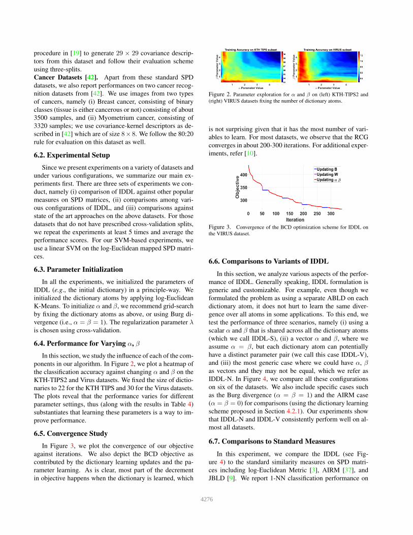
6.4. Performance for Varying α, β

In this section, we study the influence of each of the com-

ponents in our algorithm. In Figure 2, we plot a heatmap of

the classification accuracy against changing α and β on the

KTH-TIPS2 and Virus datasets. We fixed the size of dictio-

naries to 22 for the KTH TIPS and 30 for the Virus datasets.

The plots reveal that the performance varies for different

parameter settings, thus (along with the results in Table 4)

substantiates that learning these parameters is a way to im-

prove performance.

6.5. Convergence Study

In Figure 3, we plot the convergence of our objective

against iterations. We also depict the BCD objective as

contributed by the dictionary learning updates and the pa-

rameter learning. As is clear, most part of the decrement

in objective happens when the dictionary is learned, which

Figure 2. Parameter exploration for α and β on (left) KTH-TIPS2 and

(right) VIRUS datasets fixing the number of dictionary atoms.

is not surprising given that it has the most number of vari-

ables to learn. For most datasets, we observe that the RCG

converges in about 200-300 iterations. For additional exper-

iments, refer [10].

Figure 3. Convergence of the BCD optimization scheme for IDDL on

the VIRUS dataset.

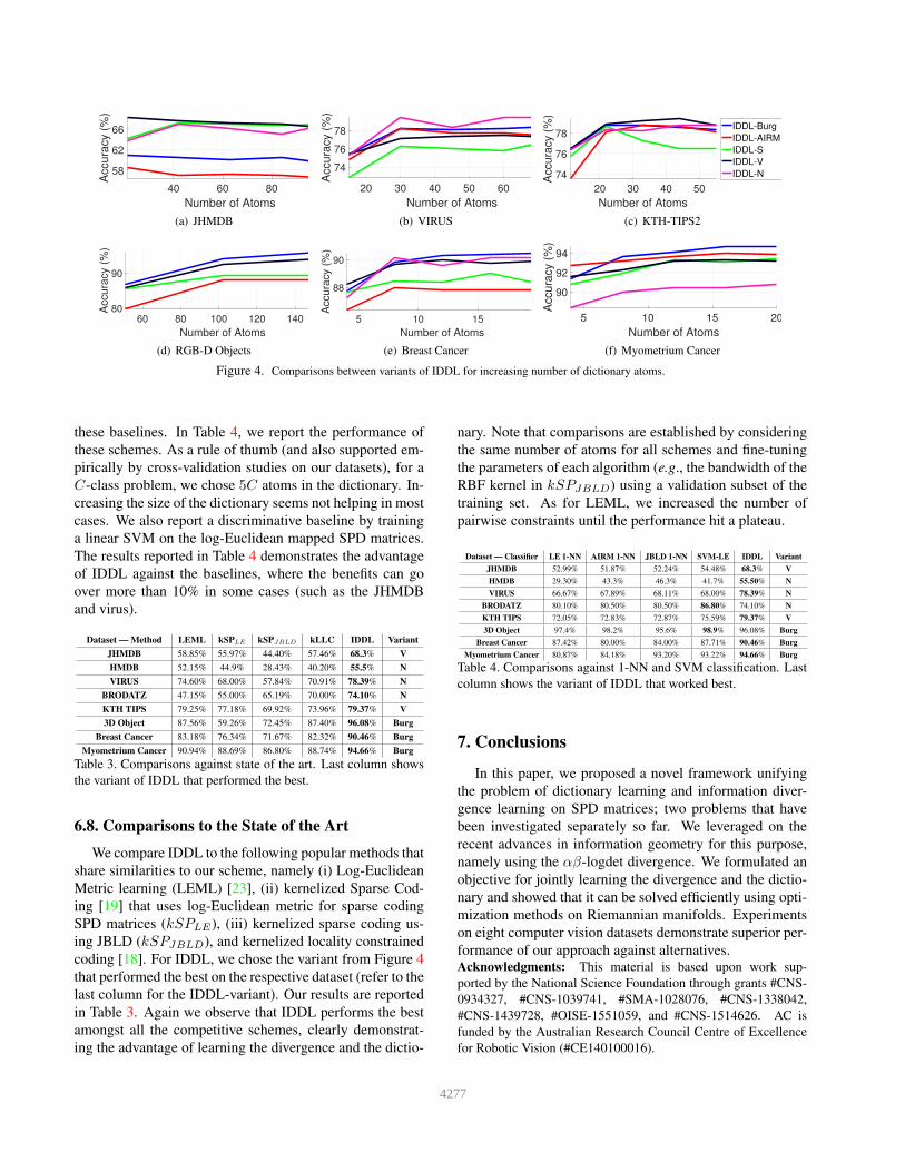
6.6. Comparisons to Variants of IDDL

In this section, we analyze various aspects of the perfor-

mance of IDDL. Generally speaking, IDDL formulation is

generic and customizable. For example, even though we

formulated the problem as using a separate ABLD on each

dictionary atom, it does not hurt to learn the same diver-

gence over all atoms in some applications. To this end, we

test the performance of three scenarios, namely (i) using a

scalar α and β that is shared across all the dictionary atoms

(which we call IDDL-S), (ii) a vector α and β, where we

assume α = β, but each dictionary atom can potentially

have a distinct parameter pair (we call this case IDDL-V),

and (iii) the most generic case where we could have α, β

as vectors and they may not be equal, which we refer as

IDDL-N. In Figure 4, we compare all these configurations

on six of the datasets. We also include specific cases such

as the Burg divergence (α = β = 1) and the AIRM case

(α = β = 0) for comparisons (using the dictionary learning

scheme proposed in Section 4.2.1). Our experiments show

that IDDL-N and IDDL-V consistently perform well on al-

most all datasets.

6.7. Comparisons to Standard Measures

In this experiment, we compare the IDDL (see Fig-

ure 4) to the standard similarity measures on SPD matri-

ces including log-Euclidean Metric [3], AIRM [37], and

JBLD [9]. We report 1-NN classification performance on

4276

40 60 80

Number of Atoms

58

62

66

Accu

racy (

%)

(a) JHMDB

20 30 40 50 60

Number of Atoms

74

76

78

Accu

racy (

%)

(b) VIRUS

20 30 40 50

Number of Atoms

74

76

78

Accu

racy (

%)

IDDL-Burg

IDDL-AIRM

IDDL-S

IDDL-V

IDDL-N

(c) KTH-TIPS2

60 80 100 120 140

Number of Atoms

80

90

Accu

racy (

%)

(d) RGB-D Objects

5 10 15

Number of Atoms

88

90

Accu

racy (

%)

(e) Breast Cancer

5 10 15 20

Number of Atoms

90

92

94

Accura

cy (

%)

(f) Myometrium Cancer

Figure 4. Comparisons between variants of IDDL for increasing number of dictionary atoms.

these baselines. In Table 4, we report the performance of

these schemes. As a rule of thumb (and also supported em-

pirically by cross-validation studies on our datasets), for a

C-class problem, we chose 5C atoms in the dictionary. In-

creasing the size of the dictionary seems not helping in most

cases. We also report a discriminative baseline by training

a linear SVM on the log-Euclidean mapped SPD matrices.

The results reported in Table 4 demonstrates the advantage

of IDDL against the baselines, where the benefits can go

over more than 10% in some cases (such as the JHMDB

and virus).

Dataset — Method LEML kSPLE kSPJBLD kLLC IDDL Variant

JHMDB 58.85% 55.97% 44.40% 57.46% 68.3% V

HMDB 52.15% 44.9% 28.43% 40.20% 55.5% N

VIRUS 74.60% 68.00% 57.84% 70.91% 78.39% N

BRODATZ 47.15% 55.00% 65.19% 70.00% 74.10% N

KTH TIPS 79.25% 77.18% 69.92% 73.96% 79.37% V

3D Object 87.56% 59.26% 72.45% 87.40% 96.08% Burg

Breast Cancer 83.18% 76.34% 71.67% 82.32% 90.46% Burg

Myometrium Cancer 90.94% 88.69% 86.80% 88.74% 94.66% Burg

Table 3. Comparisons against state of the art. Last column shows

the variant of IDDL that performed the best.

6.8. Comparisons to the State of the Art

We compare IDDL to the following popular methods that

share similarities to our scheme, namely (i) Log-Euclidean

Metric learning (LEML) [23], (ii) kernelized Sparse Cod-

ing [19] that uses log-Euclidean metric for sparse coding

SPD matrices (kSPLE), (iii) kernelized sparse coding us-

ing JBLD (kSPJBLD), and kernelized locality constrained

coding [18]. For IDDL, we chose the variant from Figure 4

that performed the best on the respective dataset (refer to the

last column for the IDDL-variant). Our results are reported

in Table 3. Again we observe that IDDL performs the best

amongst all the competitive schemes, clearly demonstrat-

ing the advantage of learning the divergence and the dictio-

nary. Note that comparisons are established by considering

the same number of atoms for all schemes and fine-tuning

the parameters of each algorithm (e.g., the bandwidth of the

RBF kernel in kSPJBLD) using a validation subset of the

training set. As for LEML, we increased the number of

pairwise constraints until the performance hit a plateau.

Dataset — Classifier LE 1-NN AIRM 1-NN JBLD 1-NN SVM-LE IDDL Variant

JHMDB 52.99% 51.87% 52.24% 54.48% 68.3% V

HMDB 29.30% 43.3% 46.3% 41.7% 55.50% N

VIRUS 66.67% 67.89% 68.11% 68.00% 78.39% N

BRODATZ 80.10% 80.50% 80.50% 86.80% 74.10% N

KTH TIPS 72.05% 72.83% 72.87% 75.59% 79.37% V

3D Object 97.4% 98.2% 95.6% 98.9% 96.08% Burg

Breast Cancer 87.42% 80.00% 84.00% 87.71% 90.46% Burg

Myometrium Cancer 80.87% 84.18% 93.20% 93.22% 94.66% Burg

Table 4. Comparisons against 1-NN and SVM classification. Last

column shows the variant of IDDL that worked best.

7. Conclusions

In this paper, we proposed a novel framework unifying

the problem of dictionary learning and information diver-

gence learning on SPD matrices; two problems that have

been investigated separately so far. We leveraged on the

recent advances in information geometry for this purpose,

namely using the αβ-logdet divergence. We formulated an

objective for jointly learning the divergence and the dictio-

nary and showed that it can be solved efficiently using opti-

mization methods on Riemannian manifolds. Experiments

on eight computer vision datasets demonstrate superior per-

formance of our approach against alternatives.Acknowledgments: This material is based upon work sup-

ported by the National Science Foundation through grants #CNS-

0934327, #CNS-1039741, #SMA-1028076, #CNS-1338042,

#CNS-1439728, #OISE-1551059, and #CNS-1514626. AC is

funded by the Australian Research Council Centre of Excellence

for Robotic Vision (#CE140100016).

4277

References

[1] P.-A. Absil, R. Mahony, and R. Sepulchre. Optimization al-

gorithms on matrix manifolds. Princeton University Press,

2009. 4, 5

[2] S.-i. Amari and H. Nagaoka. Methods of information geom-

etry, volume 191. American Mathematical Soc., 2007. 2

[3] V. Arsigny, P. Fillard, X. Pennec, and N. Ayache. Log-

euclidean metrics for fast and simple calculus on diffusion

tensors. Magnetic resonance in medicine, 56(2):411–421,

2006. 1, 2, 7

[4] A. Basu, I. R. Harris, N. L. Hjort, and M. Jones. Robust

and efficient estimation by minimising a density power di-

vergence. Biometrika, 85(3):549–559, 1998. 2

[5] T. Brox, J. Weickert, B. Burgeth, and P. Mrazek. Nonlinear

structure tensors. Image and Vision Computing, 24(1):41–

55, 2006. 1

[6] J. Carreira, R. Caseiro, J. Batista, and C. Sminchisescu. Se-

mantic segmentation with second-order pooling. In ECCV,

2012. 1

[7] A. Cherian, P. Koniusz, and S. Gould. Higher-order pooling

of CNN features via kernel linearization for action recogni-

tion. In WACV, 2017. 6

[8] A. Cherian and S. Sra. Riemannian dictionary learning and

sparse coding for positive definite matrices. IEEE Trans. on

Neural Networks and Learning Systems, 2016. 2, 4, 5, 6

[9] A. Cherian, S. Sra, A. Banerjee, and N. Papanikolopou-

los. Jensen-bregman logdet divergence with application to

efficient similarity search for covariance matrices. PAMI,

35(9):2161–2174, 2013. 2, 4, 7

[10] A. Cherian, P. Stanitsas, M. Harandi, V. Morellas, and

N. Papanikolopoulos. Learning discriminative alpha-beta di-

vergences for positive definite matrices (extended version).

CoRR, –:–, 2017. 5, 7

[11] A. Cichocki and S.-i. Amari. Families of alpha-beta-and

gamma-divergences: Flexible and robust measures of sim-

ilarities. Entropy, 12(6):1532–1568, 2010. 2

[12] A. Cichocki, S. Cruces, and S.-i. Amari. Log-determinant

divergences revisited: Alpha-beta and gamma log-det diver-

gences. Entropy, 17(5):2988–3034, 2015. 2, 3

[13] A. Cichocki, R. Zdunek, A. H. Phan, and S.-i. Amari. Non-

negative matrix and tensor factorizations: applications to

exploratory multi-way data analysis and blind source sep-

aration. John Wiley & Sons, 2009. 2

[14] I. S. Dhillon and S. Sra. Generalized nonnegative matrix

approximations with bregman divergences. In NIPS, 2005. 2

[15] O. Dikmen, Z. Yang, and E. Oja. Learning the information

divergence. PAMI, 37(7):1442–1454, 2015. 2

[16] D. Fehr. Covariance based point cloud descriptors for ob-

ject detection and classification. PhD thesis, University Of

Minnesota, 2013. 6

[17] G. H. Golub and C. F. Van Loan. Matrix computations, vol-

ume 3. JHU Press, 2012. 5

[18] M. Harandi and M. Salzmann. Riemannian coding and dic-

tionary learning: Kernels to the rescue. In CVPR, 2015. 1,

3, 4, 5, 8

[19] M. Harandi, M. Salzmann, and F. Porikli. Bregman di-

vergences for infinite dimensional covariance matrices. In

CVPR, 2014. 3, 6, 7, 8

[20] M. T. Harandi, M. Salzmann, and R. Hartley. From manifold

to manifold: Geometry-aware dimensionality reduction for

spd matrices. In ECCV, 2014. 2

[21] G. Hinton and S. Roweis. Stochastic neighbor embedding.

In NIPS, 2002. 2

[22] Z. Huang and L. Van Gool. A Riemannian network for SPD

matrix learning. CoRR arXiv:1608.04233, 2016. 1

[23] Z. Huang, R. Wang, S. Shan, X. Li, and X. Chen. Log-

Euclidean metric learning on symmetric positive definite

manifold with application to image set classification. In

ICML, 2015. 2, 8

[24] C. Ionescu, O. Vantzos, and C. Sminchisescu. Matrix back-

propagation for deep networks with structured layers. In

ICCV, 2015. 1

[25] H. Jhuang, J. Gall, S. Zuffi, C. Schmid, and M. J. Black.

Towards understanding action recognition. In ICCV, 2013. 6

[26] R. Kompass. A generalized divergence measure for nonneg-

ative matrix factorization. Neural computation, 19(3):780–

791, 2007. 2

[27] H. Kuehne, H. Jhuang, E. Garrote, T. Poggio, and T. Serre.

Hmdb: a large video database for human motion recognition.

In ICCV, 2011. 6

[28] B. Kulis, M. Sustik, and I. Dhillon. Learning low-rank kernel

matrices. In ICML, 2006. 2, 4

[29] G. Kylberg, M. Uppstrom, K. Hedlund, G. Borgefors, and

I. Sintorn. Segmentation of virus particle candidates in trans-

mission electron microscopy images. Journal of microscopy,

245(2):140–147, 2012. 6

[30] J. Lafferty. Additive models, boosting, and inference for gen-

eralized divergences. In Proc. conf. on Computational learn-

ing theory, 1999. 2

[31] K. Lai, L. Bo, X. Ren, and D. Fox. A large-scale hierarchical

multi-view RGB-D object dataset. In ICRA, 2011. 6

[32] P. Li, Q. Wang, W. Zuo, and L. Zhang. Log-Euclidean ker-

nels for sparse representation and dictionary learning. In

ICCV, 2013. 3

[33] P. Mallikarjuna, A. T. Targhi, M. Fritz, E. Hayman, B. Ca-

puto, and J.-O. Eklundh. The KTH-TIPS2 database, 2006.

6

[34] M. Mihoko and S. Eguchi. Robust blind source separation

by beta divergence. Neural computation, 14(8):1859–1886,

2002. 2

[35] M. Moakher and P. G. Batchelor. Symmetric positive-

definite matrices: From geometry to applications and visu-

alization. In Visualization and Processing of Tensor Fields,

pages 285–298. Springer, 2006. 2, 4

[36] T. Ojala, M. Pietikainen, and D. Harwood. A comparative

study of texture measures with classification based on fea-

tured distributions. Pattern recognition, 29(1):51–59, 1996.

6

[37] X. Pennec, P. Fillard, and N. Ayache. A Riemannian frame-

work for tensor computing. IJCV, 66(1):41–66, 2006. 1, 2,

3, 4, 7

4278

[38] K. Simonyan and A. Zisserman. Two-stream convolutional

networks for action recognition in videos. In NIPS, 2014. 6

[39] U. Simsekli, A. T. Cemgil, and B. Ermis. Learning mixed di-

vergences in coupled matrix and tensor factorization models.

In ICASSP, 2015. 2

[40] R. Sivalingam, D. Boley, V. Morellas, and N. Papanikolopou-

los. Tensor sparse coding for region covariances. In ECCV,

2010. 2

[41] R. Sivalingam, V. Morellas, D. Boley, and N. Papanikolopou-

los. Metric learning for semi-supervised clustering of region

covariance descriptors. In ICDSC, 2009. 2

[42] P. Stanitsas, A. Cherian, X. Li, A. Truskinovsky, V. Morellas,

and N. Papanikolopoulos. Evaluation of feature descriptors

for cancerous tissue recognition. In ICPR, 2016. 7

[43] D. B. Thiyam, S. Cruces, J. Olias, and A. Cichocki. Opti-

mization of alpha-beta log-det divergences and their applica-

tion in the spatial filtering of two class motor imagery move-

ments. Entropy, 19(3):89, 2017. 2

[44] O. Tuzel, F. Porikli, and P. Meer. Region covariance: A fast

descriptor for detection and classification. In ECCV, 2006. 1

[45] L. Wang, J. Zhang, L. Zhou, C. Tang, and W. Li. Beyond co-

variance: Feature representation with nonlinear kernel ma-

trices. In ICCV, 2015. 1

[46] R. Wang, H. Guo, L. S. Davis, and Q. Dai. Covariance dis-

criminative learning: A natural and efficient approach to im-

age set classification. In CVPR, 2012. 2

[47] Y. Xie, J. Ho, and B. Vemuri. On a nonlinear generalization

of sparse coding and dictionary learning. In ICML, 2013. 2

4279