Large liquidity expansion of super-hedging costs

Dylan Possamai ∗ H. Mete Soner† Nizar Touzi‡

August 28, 2010

Abstract

We consider a financial market with liquidity cost as in Cetin, Jarrow and Protter[3] where the supply function Sε(s, ν) depends on a parameter ε ≥ 0 with S0(s, ν) = s

corresponding to the perfect liquid situation. Using the PDE characterization of Cetin,Soner and Touzi [6] of the super-hedging cost of an option written on such a stock, weprovide a Taylor expansion of the super-hedging cost in powers of ε. In particular, weexplicitly compute the first term in the expansion for a European Call option and givebounds for the order of the expansion for a European Digital Option.

Key words: Super-replication, liquidity, viscosity solutions, asymptotic expansions.

AMS 2000 subject classifications: 91B28, 35K55, 60H30.

∗CMAP, Ecole Polytechnique Paris, dylan.possamai@polytechnique.edu.†ETH (Swiss Federal Institute of Technology), Zurich, hmsoner@ethz.ch. Research partly supported by

the European Research Council under the grant 228053-FiRM.‡CMAP, Ecole Polytechnique Paris, nizar.touzi@polytechnique.edu. Research supported by the Chair

Financial Risks of the Risk Foundation sponsored by Societe Generale, the Chair Derivatives of the Fu-

ture sponsored by the Federation Bancaire Francaise, and the Chair Finance and Sustainable Development

sponsored by EDF and Calyon.

1

1 Introduction

The classical option pricing equation of Black & Scholes is derived under several simplifyingassumptions. The “infinite” liquidity of the underlying stock process is one of them. Inan attempt to understand the impact of liquidity, Cetin, Jarrow, Protter and collaborators[3, 4, 5] postulated the existence of a supply curve S(t, s, ν) which is the price of a share ofthe stock when one wants to buy ν shares at time t. In the Black & Scholes setting, thisprice function is taken to be independent of ν corresponding to infinite amount of supply,hence infinite liquidity. In a recent paper, Cetin, Soner and Touzi [6] used this model andstudied the liquidity premium in the price of an option written on such a stock with lessthan infinite liquidity. They characterized the option price by a nonlinear Black & Scholesequation, given in (2.3) below. In this pricing equation the liquidity manifests itself bymeans of a liquidity function `, which is given by

`(t, s) :=[4∂S∂ν

(t, s, 0)]−1

, (t, s) ∈ [0, T ]× R+.

The liquidity function ` measures the level of liquidity of the market. Namely, the larger `is, the more liquid the market is.

The main result of [6] is the characterization of the liquidity premium as the uniqueviscosity solution of a nonlinear Black-Scholes equation (2.3), which is very similar tothe one derived by Barles and Soner [2]. This nonlinear equation can only be solvednumerically as no explicit solutions are available. Motivated by this fact, in this paper weobtain rigorous asymptotic expansions for the liquidity premium. For vanilla options withsufficiently regular payoff, this expansion can be calculated explicitly giving further insightinto the liquidity effects.As stated the chief objective of this paper is to analyze the large liquidity effect. Thus, weassume that the supply function depends on a small parameter ε

Sε(t, s, ν) := S(t, s, εν), (t, s) ∈ [0, T ]× R+.

Then, the corresponding liquidity function is given by

`ε(t, s) :=1ε`(t, s), (t, s) ∈ [0, T ]× R+ .

Hence, as ε tends to zero, the market becomes completely liquid. So we expect the priceof an option V ε to converge to the classical Black-Scholes price, vBS , and we are interestedin expansions of the form

V ε = vBS + εv(1) + . . .+ εnv(n) + +o(εn).

Indeed, we prove this type of results and identify the functions v(n) in some cases. Inparticular, we show that

v(1)(t, s) =∫ T

tEt,s

[S2uσ

2(u, Su)4`(u, Su)

(vBSss (u, Su)

)2]du. (1.1)

This is exactly the liquidity premium of the standard Black-Scholes hedge.

2

The paper is organized as follows. The problem is introduced in the next section and theapproach is formally introduced in Section 3. Under a strong smoothness assumption, fullexpansion is obtained in Section 4. A quick convergence result is proved in Section 5. TheCall option is studied in Section 6 and the Digital option in the final section.

2 The general setting

Let (Ω,F ,P) be a complete probability space endowed with a Brownian motion W withcompleted canonical filtration F = Ft, t ∈ [0, T ], where T > 0 is fixed maturity. Themarginal price process St is defined by the stochastic differential equation

dStSt

= σ(t, St)dWt,

where σ is assumed to be bounded, Lipschitz-continuous and uniformly elliptic.Given a continuous portfolio strategy Y with finite quadratic variation process 〈Y 〉, thesmall time liquidation value of the portfolio is given by

dZε,Yt = YtdSt − [4`ε(t, St)]−1 d〈Y 〉t = YtdSt − ε [4`(t, St)]

−1 d〈Y 〉t.

The dependence of the process Z on its initial condition is suppressed for simplicity.Given a function g : R+ −→ R satisfying

g is bounded from below and sups>0

g(s)1 + s

< ∞, (2.1)

the super-hedging cost is defined by

V ε(t, s) := infz : Zε,Yt = z and Zε,YT ≥ g (ST ) P-as for some Y ∈ At,s

, (2.2)

where the time origin is removed to t and the initial condition for the price process is St = s.We refer to [6] for the precise definition of the set of admissible strategies At,s.This problem is similar to the super-replication problem studied extensively in [7, 8, 9,17, 18, 19, 20]. In the above setting, it is shown in Cetin, Soner and Touzi [6] that thevalue function of the super-hedging problem is the unique viscosity solution of the followingnonlinear equation,

−V εt + Hε (t, s, V ε

ss) = 0, on [0, T )× (0,∞), (2.3)

satisfying the terminal condition V ε(T, .) = g and the growth condition

−C ≤ V ε(t, s) ≤ C(1 + s), (t, s) ∈ [0, T ]× R+, for some constant C > 0 . (2.4)

Here, Hε denotes the elliptic majorant of the first guess operator Hε:

Hε(t, s, γ) := supβ≥0

Hε(t, s, γ + β),

Hε(t, s, γ) := −12s2σ2(t, s)γ − ε[4`(t, s)]−1s2σ2(t, s)γ2.

3

By direct calculation, it follows that

Hε(t, s, γ) = −12s2σ2(t, s)

γ +(γ +

`(t, s)ε

)−+

ε

2`(t, s)

(γ +

(γ +

`(t, s)ε

)−)2 .

For ε = 0, both Hε, Hε coincides with the following standard elliptic operator,

H0(t, s, γ) = H0(t, s, γ) = −12s2σ2(t, s)γ, (t, s, γ) ∈ [0, T ]× R+ × R.

Hence, the equation (2.3) reduces to the linear Black-Scholes equation

−∂vBS

∂t− 1

2s2σ2(t, s)vBSss = 0. (2.5)

We recall the well-known fact that its unique solution, vBS , is the Black-Scholes price,

vBS(t, s) = Et,s [g(ST )] , (t, s) ∈ [0, T ]× R+,

where we used the notation Et,s = E[ · | St = s].

3 Formal calculations and Assumptions

It is formally clear that as the market becomes more liquid, V ε should converge to theBlack-Scholes price vBS . Indeed, this is proved in Section 5. We are also interested in aTaylor expansion of V ε in the parameter ε, i.e.,

V ε(t, s) = vBS(t, s) + εv(1)(t, s) + ε(2)v2(t, s) + . . .+ εnv(n)(t, s) + o(εn), (3.1)

where o(εn) is the standard notation, indicating that o(εn)/εn converges to zero as ε tendsto zero.Indeed, under sufficient regularity

v(n)(t, s) =1n!

∂nV ε(t, s)∂εn

∣∣∣∣ε=0

.

Thus, formally differentiate the equation (2.3) n-times with respect to ε and then set ε tozero. Using the above formal definition of v(n), we arrive at,

0 = −v(n)t − 1

2s2σ2(t, s)v(n)

ss − Fn(t, s), (3.2)

Fn(t, s) =s2σ2(t, s)4`(t, s)

n−1∑k=0

[v(k)ss (t, s) v(n−1−k)

ss (t, s)], (3.3)

where we set v(0) := vBS . For all n ≥ 1, the terminal data is v(n)(T, ·) ≡ 0, so that theFeymann-Kac formula yields

v(n)(t, s) =n−1∑k=0

Et,s[∫ T

t

(S2uσ

2

4`v(k)ss v

(n−1−k)ss

)(u, Su)du

]. (3.4)

4

In particular, v(1) is given as in (1.1).The above calculations yield a rigorous proof when the pay-off is sufficiently regular. Wewill prove this in Section 4. On the other hand, for some discontinuous pay-offs the abovefunctions may not be finite. For instance, for a digital option, v(1) ≡ ∞. Indeed, if we take

g(s) := 1s≥K , σ(t, s) ≡ σ and `(t, s) ≡ `,

we compute that

v(1)(t, s) =1

8π`σ2

∫ T

t

(u− t)e−“

1σ√T+u−2t

ln( sK )+σ

2T−2u+t√T+u−2t

”2

(T − u)32 (T + u− 2t)

32

+1

8π`σ2

∫ T

t

e−

“1

σ√T+u−2t

ln( sK

)+σ2T−2u+t√T+u−2t

”2

√T − u(T + u− 2t)

32

(ln(sK

)σ√T + u− 2t

+σ

2T − 2u+ t√T + u− 2t

)2

.

The first term above is actually +∞ because of the non-integrability of (T − u)−3/2 nearT .

In such cases, the expansion is not valid and a careful study of the behavior of V ε near theterminal data is needed. This will be done in Section 7. However, we first prove the fullexpansion in the ”smooth” case. Then, in Section 6, we consider the Call option provingthe expansion up to n = 2. Clearly, this later result extends to all Put options. Also,remarks on other payoffs and higher expansions are given in Remarks 6.2 and 6.1.

4 Expansion for smooth pay-offs

In this section, we prove the expansion under the assumption that there is a constant C sothat

−C ≤ v(n)(t, s) ≤ C(1 + s),∣∣∣(s2 + 1)v(n)

ss (t, s)∣∣∣ ≤ C, (4.1)

|Fn(t, s)| ≤ C, ∀ (t, s) ∈ [0, T ]× R+, n = 1, 2, . . . .

Clearly, this is an implicit assumption on the pay-off g. Essentially, it holds for all smoothpay-offs growing at most linearly. In particular, (4.1) holds if σ(t, s) ≡ σ, `(t, s) ≡ ` and ifthere exists a constant C so that

−C ≤ g(s) ≤ C(1 + s),∣∣∣∣(s2 + 1)

∂n

∂sng(s)

∣∣∣∣ ≤ C, ∀ s ∈ R+, n = 2, 3, . . . .

This is proved by using the homogenity of the Black-Scholes equation and differentiatingit repeatedly.Following the techniques developed in the papers [13, 11, 14, 15, 16], for an integer n ≥ 0we define,

V ε,n(t, s) :=V ε(t, s)−

∑n−1k=0 ε

kv(k)(t, s)εn

, (4.2)

where as before we set v(0) = vBS .

5

Theorem 4.1 Assume (4.1). Then, for every n = 1, 2, . . ., there are constants Cn andε0 > 0 so that for every ε ∈ (0, ε0], and n = 1, 2, . . .,

vBS(t, s) ≤ V ε(t, s) ≤ vε,n(t, s) :=n−1∑k=0

[εkv(k)(t, s)] + εnCn(T − t). (4.3)

In particular, as ε ↓ 0, V ε converges to the Black-Scholes price vBS uniformly on compactsets. Moreover, for every n ≥ 1, V ε,n converges to v(n), again uniformly on compact sets.

Proof. Clearly, vBS ≤ V ε. We continue by proving the upper bound. Let vε,n be as in(4.3) with a constant Cn to be determined below. Using (3.2), we calculate that

−vε,nt (t, s) + Hε(t, s, vε,nss (t, s)) ≥ −vε,nt (t, s) +Hε(t, s, vε,nss (t, s))

= −vε,nt −12s2σ2vε,nss −

εs2σ2

4`(t, s)(vε,nss )2

= εnCn +n−1∑k=1

[εk Fk(t, s)]−εs2σ2

4`(t, s)(vε,nss )2 .

In view of (3.3),

εs2σ2

4`(t, s)(vε,nss )2 −

n−1∑k=1

[εk Fk(t, s)] = εnFn(t, s) + εn+1 s2σ2

4`(t, s)gε(t, s),

where gε(t, s) is a quadratic function v(k)ss (t, s) for k ≤ n and possibly powers of ε. Hence

by (4.1), there is a constant Cn,∣∣∣∣∣n−1∑k=1

[εk Fk(t, s)]−εs2σ2

4`(t, s)(vε,nss )2

∣∣∣∣∣ ≤ εnCn.Hence, we conclude that vε,n is a supersolution of (2.3). Moreover, by (4.1), −C ≤vε,n(t, s) ≤ C(1 + s). Then, by the comparison theorem for (2.3) (Theorem 6.1 of [6]),we conclude that V ε(t, s) ≤ vε,n(t, s).In particular, this estimate implies the convergence of V ε to vBS . To prove the convergenceof V ε,n, we first observe that

V ε =n∑k=0

[εkv(n)(t, s)] + εnV ε,n.

Using the equations (2.3) and (3.2), we conclude that V ε,n is a viscosity solution of

−V ε,nt − 1

2s2σ2(t, s)V ε,n

ss + F ε,n (t, s, V ε,nss ) = 0, (t, s) ∈ [0, T )× R+,

where

F ε,n(t, s, γ) :=1εn

[Hε(t, s, vε,nss (t, s) + εnγ) +

12s2σ2vε,nss +

n−1∑k=1

εkF k(t, s)

].

6

Tedious but a straightforward calculation shows that

lim(t′,s′,γ′,ε)→(t,s,γ,0)

F ε,n(t′, s′, γ′) = Fn(t, s),

where Fn is as in (3.3). Then, by the classical stability results of viscosity solutions [1, 10,12], the Barles-Perthame semi-relaxed limits

v(n)(t, s) := lim inf(t′,s′,ε)→(t,s,0)

V ε,n(t′, s′) and v(n)(t, s) := lim sup(t′,s′,ε)→(t,s,0)

V ε,n(t′, s′),

are, respectively, a viscosity supersolution and a subsolution of the equation (3.2) satisfiedby v(n). Moreover it follows from (4.3) that

v(n)(T, ·) = v(n)(T, ·) = 0 = v(n)(T, ·).

We now use the comparison result for the linear partial differential equation (3.2), andconclude that v(n) ≥ v(n). Since

v(n)(t, s) ≤ lim infε→0

V ε,n(t, s) ≤ lim supε→0

V ε,n(t, s) ≤ v(n)(t, s)

on [0, T ] × R+, this proves that v(n) = v(n) = v(n). Hence, V ε,n converges to the uniquesolution v(n), uniformly on compact sets.

2

5 A general convergence result

In this section, we prove an easy convergence result under the following general assumption.We assume that

cs2 ≤ `(t, s), (5.1)

for some constant and

Assumption 5.1 There is a decreasing sequence of smooth approximation gm ≥ g of thepay-off g satisfying (4.1) with n = 1, 2. Let v(n)

m , Fnm be the previously defined functionswith pay-off gm. Then, F 1

m(t, s) ≤ cm for some constant cm.

This assumption is satisfied by all Lipschitz or for all bounded pay-offs.

Theorem 5.1 Assume (2.1), (5.1) and that Assumption 5.1 holds true. Then, as theliquidity parameter goes to infinity, or equivalently as ε ↓ 0, V ε converges to the Black-Scholes price vBS.

Proof. Let cm be as above and set

uε(t, s) := vBSm (t, s) + εcm(T − t).

7

As in the proof of Theorem 4.1, we can show that uε is a super-solution of (2.3). Hence,V ε ≤ uε. Therefore,

lim supε↓0

V ε(t, s) ≤ vBSm (t, s).

By (2.1), vBSm (t, s) converges to vBS(t, s). Since V ε ≥ vBS , this proves the convergence ofV ε to vBS .

2

6 First order expansion for convex payoffs

One major limitation of our previous result is that the Call pay-off does not satisfy theAssumption (4.1). Therefore, in this section, we prove the first term in the Taylor expansion(3.1), i.e.,

V ε(t, s) = vBS(t, s) + εv(1)(t, s) + o(ε), (6.1)

for convex payoffs satisfying weaker assumptions than (4.1). In particular, we will showthat call options verify those assumptions.

6.1 The general result

In order to capitalize on the results we have already obtained for smooth payoffs, we willalso consider a regularized version of our problem

−V ε,αt + Hε(t, s, V ε,α

ss ) = 0, for (t, s) ∈ [0, T )× R+,

V ε,α(T, s) = gα(s), (6.2)

where gα(s) = φα ∗ g(s) with φα(·) := 1αφ( ·α) and φ is a positive, symmetric bump function

on R, compactly supported in [−1, 1] and satisfying∫ 1

−1φ(u)du = 1.

By convexity of g, for all α > 0 we have gα ≥ g, so that by monotony of our problem

V ε ≤ V ε,α.

Thus, since the main idea of our proof is to find a super-solution of (2.3), we see that it isenough to find a super-solution of (6.2). Let vBS,α and v(1),α, respectively, be the Black-Scholes price and the first-order expansion term for the regularized option. We now stateour assumptions

Assumption 6.1 (i) vBS + vBS,α + v(1) + v(1),α < +∞.

8

(ii) As α tends to 0 we have

vBS,α(t, s) = vBS(t, s) +O(α2),

v(1),α(t, s) = v(1)(t, s) + o(1).

(iii) There exists a constant c∗ independent of s, T − t and α and (ν, β) ∈ [0, 1]× [1/2, 1]such that 1 < 2β + ν < 2 and

s2σ2

4`(v(1),αss (t, s))2 ≤ c∗

(T − t)1−να2+2ν, s

∣∣vBS,αss (t, s)∣∣ ≤ c∗

(T − t)1−βα2β−1.

This assumption will be proved to be verified by Call options payoffs in subsection 6.2.

Let V ε,1 be as (4.2), i.e.

V ε,1(t, s) :=V ε(t, s)− vBS(t, s)

ε.

Theorem 6.1 Let Assumption 6.1 hold true and let a ∈ (12 ,

12β+ν ). Then for every (t, s) ∈

[0, T ]× R+ we have,

vBS ≤ V ε ≤ vBS,εa + εv(1),εa + c∗(T − t)β+ ν−12 ε2−a(ν+2β) + c∗(T − t)νε3−2a(1+ν).

Moreover, V ε → vBS, V ε,1 → v(1) uniformly on compact sets, and (6.1) holds true.

Proof. It is clear that V ε ≥ vBS . To prove the reverse inequality, we start by following atechnique similar to the one used in the proof of Theorem 4.1. Set

vε,2 := vBS,εa

+ εv(1),εa + c∗(T − t)β+ ν−12 ε2−a(ν+2β) + c∗(T − t)νε3−2a(1+ν).

We calculate that for (t, s) ∈ [0, T )× R+

− vε,2t + Hε(t, s, vε,2ss ) ≥ −vε,2t +Hε(t, s, vε,2ss )

=c∗ε

2−a(ν+2β)

(T − t)1−β−ν−12

+c∗ε

3−2a(1+ν)

(T − t)1−ν− vBS,ε

a

t − εv(1),εa

t − 12s2σ2vε,2ss −

εs2σ2

4`(vε,2ss)2

=c∗ε

2−a(ν+2β)

(T − t)1−β−ν−12

+c∗ε

3−2a(1+ν)

(T − t)1−ν− s2σ2

4`(v(1),εa

ss )2ε3 − s2σ2

2`vBS,ε

a

ss v(1),εa

ss ε2.

In view of Assumption 6.1(iii), this quantity is always positive. We now analyze the terminalcondition. In view of the conditions imposed on a, β and ν

vε,2(T, s) = vBS,εa(T, s) = gεa(s).

Hence, vε,2 is a super-solution of (6.2) and therefore of (2.3). Then, by the comparisontheorem for (2.3) (proved in [6]), we conclude that V ε(t, s) ≤ vε,2(t, s).

We now let ε go to 0 in the above inequalities. This proves that V ε converges to vBS

uniformly on compact sets.

Finally, by Assumption 6.1(ii)

0 ≤ V ε,1(t, s) ≤ v(1)(t, s) + o(εmin1−a(2β+ν),2−2a(1+ν)

)+O

(ε2a−1

),

9

where it is clear with our conditions on a, β and ν that the o(·) and O(·) above go to 0 asε tends to 0.

Using this estimate, we then prove the convergence of V ε,1 exactly as in Theorem 4.1. 2

Remark 6.1 Higher expansions can be proved similarly, provided that we extend Assump-tion 6.1 for n ≥ 2.

6.2 Expansion for the Call option

In this section, we take

g(s) = (s−K)+, σ(t, s) ≡ σ, `(t, s) ≡ `,

and we verify that Assumptions 6.1(ii) and 6.1(iii) are satisfied, since Assumption 6.1(i) istrivial.

Straightforward but tedious calculations using the Feynman-Kac formula yield

vBS,αss (t, s) =1

σs√

2πτ

∫ 1

−1φ(u) exp

(−1

2d1(s,K + αu, τ)2

)du,

v(1),α(t, s) =1

8`π

∫ τ

0

∫ 1

−1

∫ 1

−1

φ(x)φ(y)hα(τ, v, s,K, x, y)√v(2τ − v)

dxdydv,

where

τ = T − t,

d1(s, k, t) =1σ√t

ln(s/k) +12σ√t,

δ(τ, v, s, k) =1

σ√

2τ − vln(s/k)− σ

2τ − 2v√2τ − v

,

hα(τ, v, s, k, x, y) = exp(−δ(τ, v, s, k)2 +

δ(τ, v, s, k)σ√

2τ − v

(log(

1 +αx

k

)+ log

(1 +

αy

k

)))× exp

(− τ

2σ2v(2τ − v)

(log(

1 +αx

k

)− log

(1 +

αy

k

))2)

× exp(− 1σ2(2τ − v)

log(

1 +αx

k

)log(

1 +αy

k

)).

The following two propositions, whose proof is relagated to the appendix, ensure thatAssumptions 6.1(ii) and 6.1(iii) are satisfied

Proposition 6.1 There exists a constant c∗, independent of s, τ and α so that for all(ν, β) ∈ [0, 1]× [1/2, 1]:

s∣∣vBS,αss (t, s)

∣∣ ≤ c∗τ1−βα2β−1

,s2σ2

4`(v(1),αss (t, s))2 ≤ c∗

τ1−να2+2ν.

10

Proposition 6.2 As α tends to 0 we have the following expansions

vBS,α(t, s) = vBS(t, s) + α2 e− 1

2d0(s,K,τ)2

2Kσ√

2πτ

∫ 1

−1φ(v)v2dv +O(α4),

v(1),α(t, s) = v(1)(t, s)− αe− 1

2d0(s,K,τ)2

8Kσ`√

2πτ

∫ 1

−1

∫ 1

−1φ(x)φ(y)|x− y|dxdy + o(α),

where d0(s, k, τ) = 1σ√τ

ln(s/k)− 12σ√τ .

Remark 6.2 It is not hard to show that the results of Propositions 6.1 and 6.2 hold for allconvex linear combination of call or put options. However, we cannot use the above prooffor, say, a call spread option whose payoff is neither convex nor concave.

6.3 Numerical Experiments

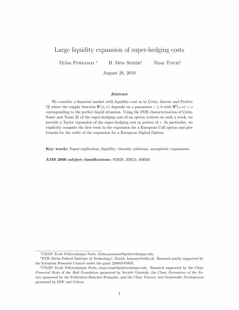
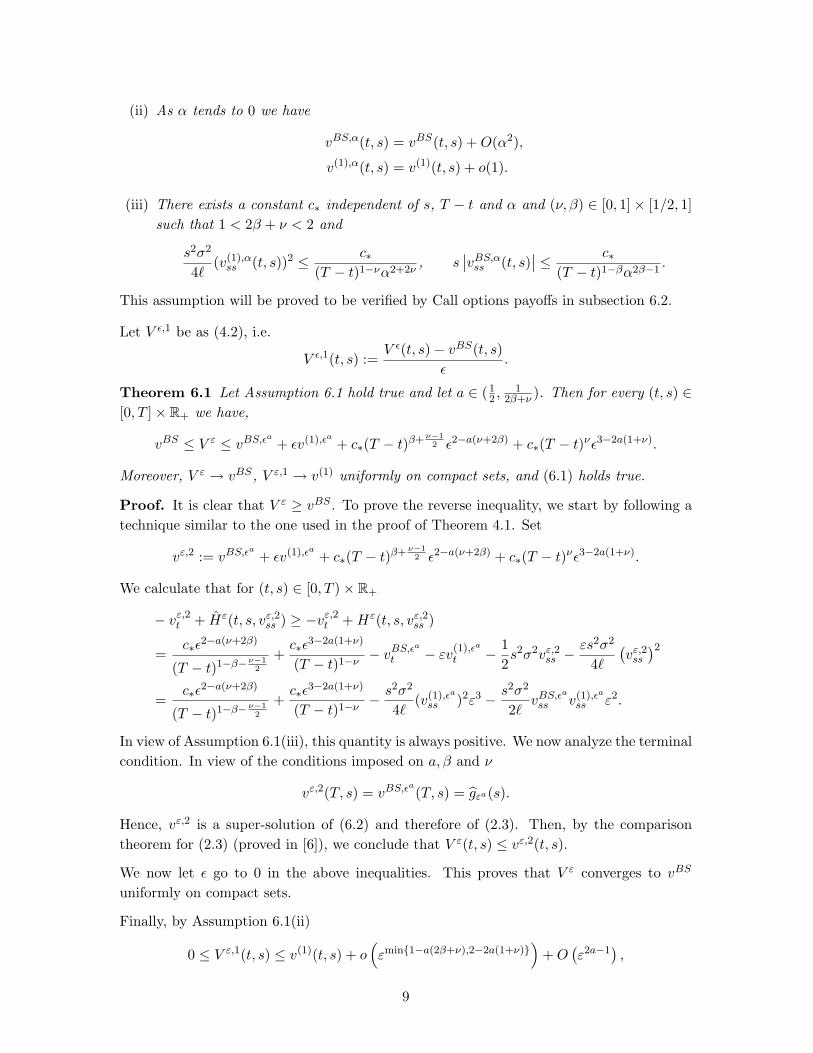
In order to have a better grasp of the liquidity effects, we also solved numerically (withsimple finite difference methods) the PDE (2.3). We represent below the behaviour of theliquidity premium (that is to say V ε−vBS) when the time to maturity t and the spot pricevary

Figure 1: Call liquidity premium - T = 10, K = 15, σ = 0.5, ε = 0.1, ` = 1

In the above figure, the liquidity effect is strongly marked for ATM options and disapearsquickly for ITM and OTM options. This was to be expected. Indeed, our calculations

11

showed that the liquidity effect is, for the first order, driven by the Γ of the call option(see (A.1)), which explodes for ATM options near maturity. Moreover, with our set ofparameters, the first order correction is at most 0.06 for a BS price of 8.56, which meansthat the hedge against liquidity risk is not that expensive when the illiquidity is not toostrong.

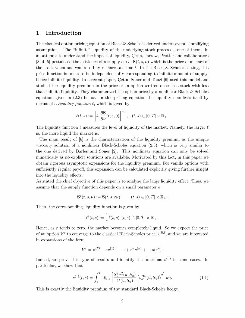
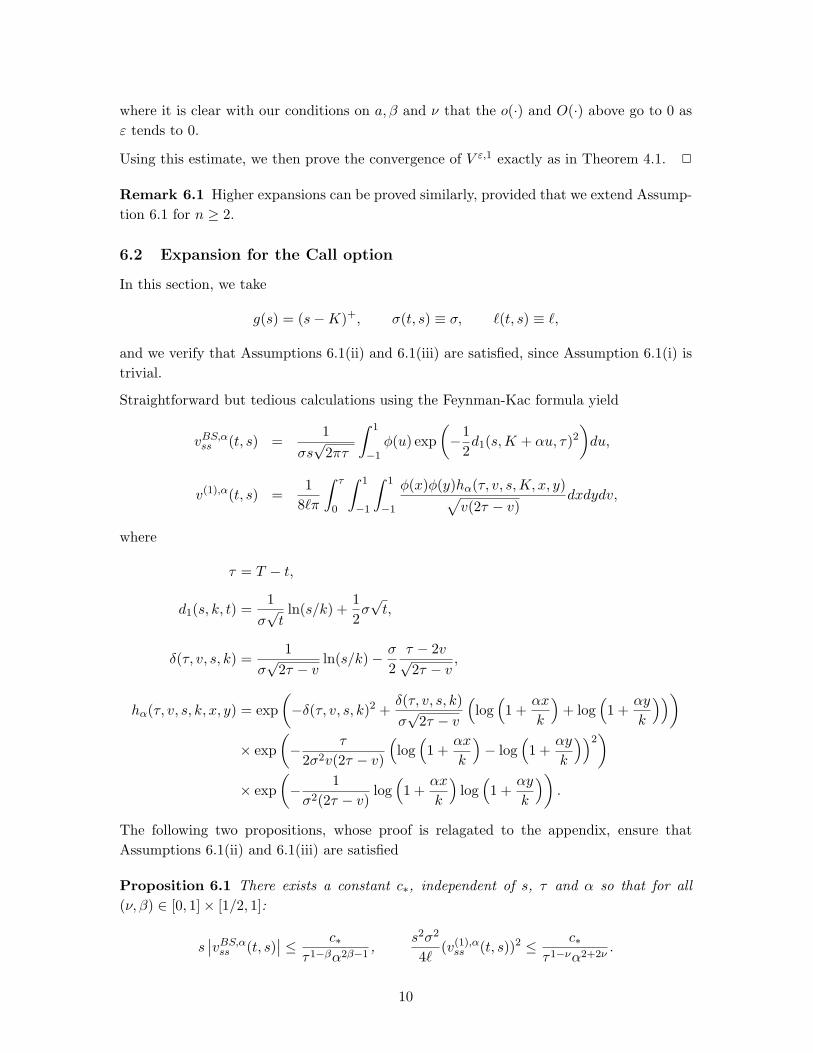
We now compare the real liquidity premium with its first-order expansion term.

Figure 2: Call first order liquidity premium - T = 10, K = 15, σ = 0.5, ε = 0.1, ` = 1

A rapid examination of the above figure shows that the first order approximation remainsexcellent as long as we do not go too far from the maturity time T and we stay close to themoney s = K. Otherwise, the first order overvalues the liquidity premium.

7 Digital Option

In this section, we analyze the specific example of a Digital option in the context of Black-Scholes model with constant liquidity parameter

g(s) := 1s≥K , and σ(t, s) ≡ σ, `(t, s) ≡ `.

12

7.1 Theoretical bounds

As pointed out earlier, for the Digital option, the first-order term that we obtained formallyis equal to +∞. Thus, the expansion (3.1) is no longer valid and our aim in this section isto find bounds for the first-order of the expansion. We start by approximating the optionby a sequence of regularized call spreads. Then the original problem (2.3) is replaced by

−V ε,αt + Hε(t, s, V ε,α

ss ) = 0, for (t, s) ∈ [0, T )× R+,

V ε,α(T, s) = gα(s), (7.1)

where gα(s) = φα ∗ gα(s) with gα(s) = (s−K+2α)+−(s−K+α)+

α .

Since φα has compact support in [−α, α], notice that gα ≥ g. Then, since the terminalcondition is smooth, it follows from the comparison principle that

V ε(t, s) ≤ V ε,α(t, s), for (t, s, α) ∈ [0, T ]× R+ × R∗+. (7.2)

With the same notations as in the previous section, we directly calculate using again theFeynman-Kac formula that

vBS,αss (t, s) =1

σsα√

2πτ

∫ 1

−1φ(u)

(e−

12d1(s,K+αu−2α,τ)2 − e−

12d1(s,K+αu−α,τ)2

)du,

v(1),α(t, s) =1

8`πα2

∫ τ

0

∫ 1

−1

∫ 1

−1

φ(x)φ(y)hα(τ, v, s,K, x, y)√v(2τ − v)

dxdydv,

where

hα(τ, v, s,K, x, y) =∑

1≤i,j≤2

hα(τ, v, s,K, x− i, y − j).

Then, we have the two following propositions which are proved exactly as in the call optioncase (since the functions involved here are essentially the same)

Proposition 7.1 There exists a constant c∗, independent of s, τ and α so that for all(ν, β) ∈ [0, 1]× [1/2, 1]

s∣∣vBS,αss (t, s)

∣∣ ≤ c∗τ1−βα2β

,s2σ2

4`(v(1),αss (t, s))2 ≤ c∗

τ1−να6+2ν.

Proposition 7.2 As α tends to 0 we have the following expansions:

vBS,α(t, s) = vBS(t, s) +32αe−

12d0(s,K,τ)2

Kσ√

2πτ+O(α2),

v(1),α(t, s) = α−1 e− 1

2d0(s,K,τ)2

8Kσ`√

2πτ

∫ 1

−1

∫ 1

−1φ(x)φ(y)(|x−y−1|+|x−y+1|−2|x−y|)dxdy + o(α−1).

13

Define V ε,1,c by

V ε,1,c(t, s) :=V ε(t, s)− vBS(t, s)

εc.

Theorem 7.1 Let (β, ν) ∈ [1/2, 1] × [0, 1] be such that γ := 2β+ν−12β+ν+4 ∈ (0, 1) and set

a := 25(1− γ). Then for all (t, s) ∈ [0, T ]× R+,

vBS ≤ V ε ≤ vBS,εa + εv(1),εa + c∗(T − t)β+ ν−12 ε2−3a−a(ν+2β) + c∗(T − t)νε3−2a(3+ν).

In particular, V ε converges to vBS, uniformly on compact sets and

0 ≤ lim inf(t′,s′,ε)→(t,s,0)

V ε,1,a(t′, s′, a) ≤ lim sup(t′,s′,ε)→(t,s,0)

V ε,1,a(t′, s′) ≤ 32e−

12d0(s,K,τ)2

Kσ√

2πτ+c∗(T−t)

5γ2(1−γ) ,

i.e. the order of the expansion is at least 2/5.

Proof. It is clear that V ε ≥ vBS . To prove the reverse inequality, we start by following atechnique similar to the one used in the proof of Theorem 6.1. Set

vε,2 := vBS,εa

+ εv(1),εa + c∗(T − t)β+ ν−12 ε2−3a−a(ν+2β) + c∗(T − t)νε3−2a(3+ν).

We proceed exactly as in Theorem 6.1 using Proposition 7.1. The result is

−vε,2t (t, s) + Hε(t, s, vε,2ss (t, s)) ≥ 0, for (t, s) ∈ [0, T )× R+.

We now analyze the terminal condition. Since 2β + ν > 1, we have

vε,2(T, s) = vBS,εa(T, s).

Hence, vε,2 is a super-solution of (6.2) and therefore of (2.3). Then, by the comparisontheorem for (2.3) (proved in [6]), we conclude that V ε(t, s) ≤ vε,2(t, s).Then by Proposition 7.2 and the conditions imposed on a, β and ν, we obtain easily theuniform convergence on compact sets of V ε to vBS by letting ε go to 0.Now for the first order term, we would like to use our expansions and obtain a finitemajorant for V ε,1,c with the largest possible c. It is easy to argue that c = a is the bestchoice possible. This, in turn, imposes the following condition

a ≤ min

12,

24 + 2β + ν

,3

7 + 2ν

=

24 + 2β + ν

.

Now it follows that, for all γ > 0 small enough, there are β and ν satisfying our conditionsso that 2

4+2β+ν = 25(1− γ). It suffices then to take the lim inf and lim sup in the inequality

to prove the result. 2

14

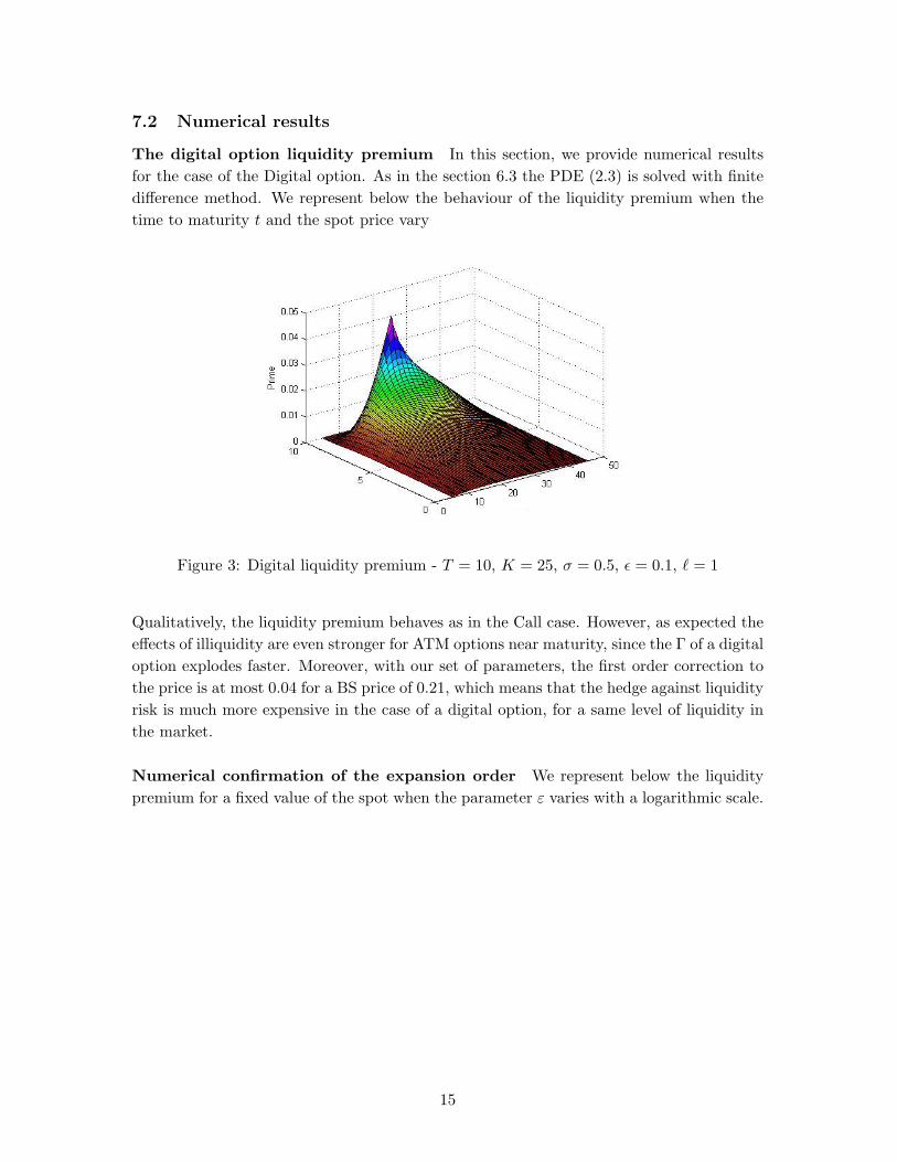
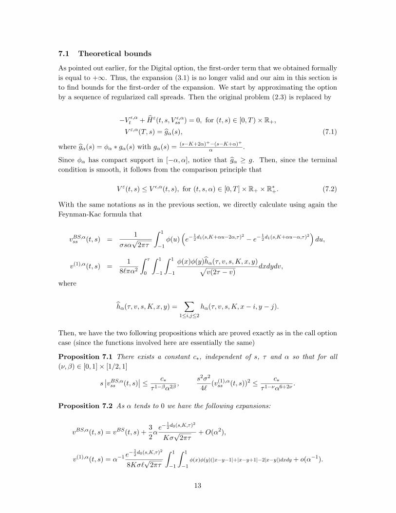
7.2 Numerical results

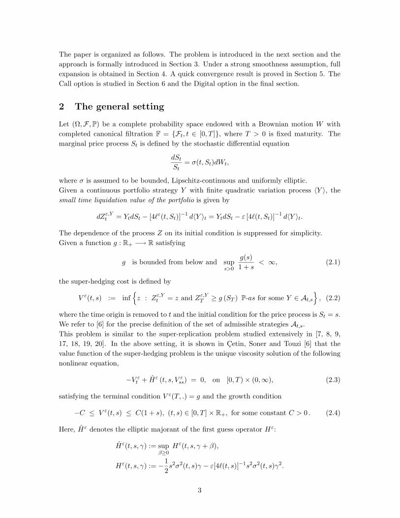
The digital option liquidity premium In this section, we provide numerical resultsfor the case of the Digital option. As in the section 6.3 the PDE (2.3) is solved with finitedifference method. We represent below the behaviour of the liquidity premium when thetime to maturity t and the spot price vary

Figure 3: Digital liquidity premium - T = 10, K = 25, σ = 0.5, ε = 0.1, ` = 1

Qualitatively, the liquidity premium behaves as in the Call case. However, as expected theeffects of illiquidity are even stronger for ATM options near maturity, since the Γ of a digitaloption explodes faster. Moreover, with our set of parameters, the first order correction tothe price is at most 0.04 for a BS price of 0.21, which means that the hedge against liquidityrisk is much more expensive in the case of a digital option, for a same level of liquidity inthe market.

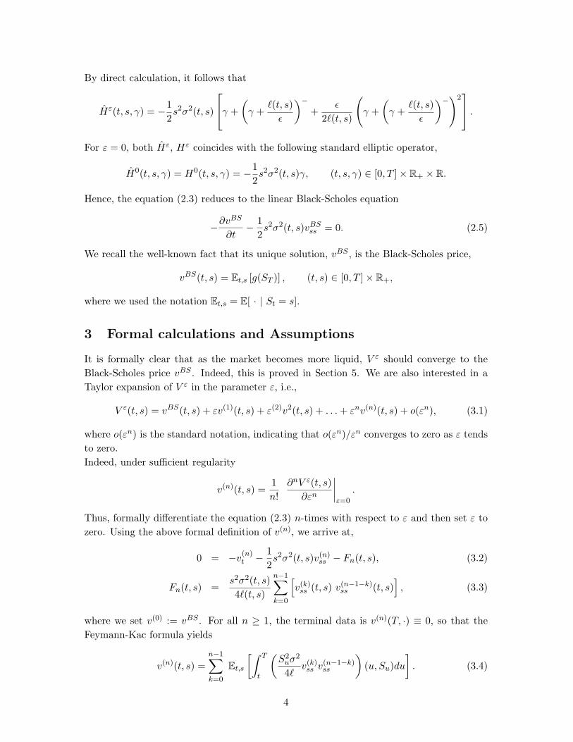
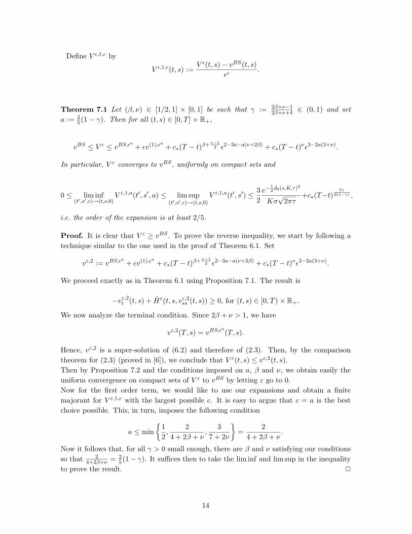
Numerical confirmation of the expansion order We represent below the liquiditypremium for a fixed value of the spot when the parameter ε varies with a logarithmic scale.

15

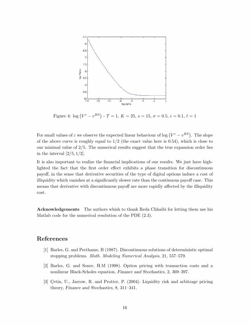
Figure 4: log(V ε − vBS

)- T = 1, K = 25, s = 15, σ = 0.5, ε = 0.1, ` = 1

For small values of ε we observe the expected linear behaviour of log(V ε − vBS

). The slope

of the above curve is roughly equal to 1/2 (the exact value here is 0.54), which is close toour minimal value of 2/5. The numerical results suggest that the true expansion order liesin the interval [2/5, 1/2].

It is also important to realize the financial implications of our results. We just have high-lighted the fact that the first order effect exhibits a phase transition for discontinuouspayoff, in the sense that derivative securities of the type of digital options induce a cost ofilliquidity which vanishes at a significantly slower rate than the continuous payoff case. Thismeans that derivative with discontinuous payoff are more rapidly affected by the illiquiditycost.

Acknowledgements The authors whish to thank Reda Chhaibi for letting them use hisMatlab code for the numerical resolution of the PDE (2.3).

References

[1] Barles, G. and Perthame, B (1987). Discontinuous solutions of deterministic optimalstopping problems. Math. Modeling Numerical Analysis, 21, 557–579.

[2] Barles, G. and Soner, H.M (1998). Option pricing with transaction costs and anonlinear Black-Scholes equation, Finance and Stochastics, 2, 369–397.

[3] Cetin, U., Jarrow, R. and Protter, P. (2004). Liquidity risk and arbitrage pricingtheory, Finance and Stochastics, 8, 311–341.

16

[4] Cetin, U., Jarrow, R., Protter, P. and Warachka, M. (2006) Pricing options in anextended Black-Scholes economy with illiquidity: theory and empirical evidence,The Review of Financial Studies, 19, 493–529.

[5] Cetin, U. and Rogers, L.C.G. (2006) Modelling liquidity effects in discrete time,Math. Finance, forthcoming.

[6] Cetin, U., Soner, H.M., and Touzi, N. (2007). Options hedging for small investorsunder liquidity costs, preprint.

[7] Cheridito, P., Soner, H.M. and Touzi, N. (2005a). The multi-dimensional super-replication problem under gamma constraints, Annales de l’Institute Henri Poincare

(C) Non Linear Analysis, 22 (5): 633-666.

[8] Cheridito, P., Soner, H.M. and Touzi, N. (2005b). Small time path behavior ofdouble stochastic integrals and applications to stochastic control, Annals of Applied

Probability, 15 (4): 2472-2495.

[9] Cheridito, P., Soner, H.M., Touzi, N., and Victoir, N. (2007). Second Order Back-ward Stochastic Differential Equations and Fully Non-Linear Parabolic PDEs, Com-

munications on Pure and Applied Mathematics, 60 (7): 1081-1110.

[10] Crandall, M.G., Ishii, H., and Lions, P.L. (1992). User’s guide to viscosity solutionsof second order partial differential equations, Bull. Amer. Math. Soc. 27(1), 1–67.

[11] Fleming, W.H., and Soner, H.M. (1989). Asymptotic expansions for Markov pro-cesses with Levy generators. Applied Mathematics and Optimization , 19(3), 203–223.

[12] Fleming, W.H., and Soner, H.M. (1993). Controlled Markov Processes and Viscosity

Solutions. Applications of Mathematics 25. Springer-Verlag, New York.

[13] Fleming, W.H., and Souganidis, P.E. (1986). Asymptotic series and the method ofvanishing viscosity, Indiana University Mathemtics Journal , 35(2), 425–447.

[14] Lehoczky, J., Sethi, S.P., Soner, H.M., and Taksar, M.I. (1991). An asymptoticanalysis of hierarchical control of manufacturing systems under uncertainity. Math-

ematics of Operations Research, 16(3), 596–608.

[15] Sethi, S., Soner, H.M., Zhang, Q., and Jiang, J. (1992). Turnpike Sets and TheirAnalysis in Stochastic Production Planning Problems. Mathematics of Operations

Research, 17(4), 932–950.

[16] Soner, H.M. (1993). Singular perturbations in manufacturing. SIAM J. Control and

Opt. 31(1), 132–146.

[17] Soner, H.M., and Touzi, N. (2000). Super-replication under gamma constraints.SIAM J. Control and Opt. 39(1), 73–96.

17

[18] Soner, H.M., and Touzi, N. (2002). Stochastic target problems, dynamic program-ming and viscosity solutions, SIAM J. Control and Opt. 41, 404–424.

[19] Soner, H.M., and Touzi, N. (2002). Dynamic programming for stochastic targetproblems and geometric flows, J. European Math. Soc., 4, 201–236.

[20] Soner, H.M., and Touzi, N. (2007). The dynamic programming equation for secondorder stochastic target problems, preprint.

18

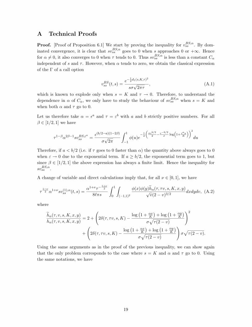
A Technical Proofs

Proof. [Proof of Proposition 6.1] We start by proving the inequality for vBS,αss . By dom-inated convergence, it is clear that svBS,αss goes to 0 when s approaches 0 or +∞. Hencefor α 6= 0, it also converges to 0 when τ tends to 0. Thus svBS,αss is less than a constant Cαindependent of s and τ . However, when α tends to zero, we obtain the classical expressionof the Γ of a call option

vBSss (t, s) =e−

12d1(s,K,τ)2

sσ√

2πτ, (A.1)

which is known to explode only when s = K and τ → 0. Therefore, to understand thedependence in α of Cα, we only have to study the behaviour of svBS,αss when s = K andwhen both α and τ go to 0.

Let us therefore take α = εa and τ = εb with a and b strictly positive numbers. For allβ ∈ [1/2, 1] we have

τ1−βα2β−1svBS,εa

ss =ε(b/2−a)(1−2β)

σ√

2π

∫ 1

−1φ(u)e

− 12

„σεb/2

2− ε−b/2σ

log“1+ εau

K

”«2

du

Therefore, if a < b/2 (i.e. if τ goes to 0 faster than α) the quantity above always goes to 0when ε → 0 due to the exponential term. If a ≥ b/2, the exponential term goes to 1, butsince β ∈ [1/2, 1] the above expression has always a finite limit. Hence the inequality forsvBS,αss .

A change of variable and direct calculations imply that, for all ν ∈ [0, 1], we have

τ1−ν2 α1+νsv(1),α

ss (t, s) =α1+ντ−

1+ν2

8`πs

∫ 1

0

∫(−1,1)2

φ(x)φ(y)hα(τ, τv, s,K, x, y)√v(2− v)3/2

dxdydv, (A.2)

where

hα(τ, v, s,K, x, y)hα(τ, v, s,K, x, y)

= 2 +

(2δ(τ, τv, s,K)−

log(1 + αx

K

)+ log

(1 + αy

K

)σ√τ(2− v)

)2

+

(2δ(τ, τv, s,K)−

log(1 + αx

K

)+ log

(1 + αy

K

)σ√τ(2− v)

)σ√τ(2− v).

Using the same arguments as in the proof of the previous inequality, we can show againthat the only problem corresponds to the case where s = K and α and τ go to 0. Usingthe same notations, we have

19

hεa(εb, εbv, s, s, x, y) = exp

−σ2εb(1− 2v)2

4(2− v)+

(1− 2v)(

log(1 + εax

K

)+ log

(1 + εay

K

))2(2− v)

× exp

(− ε−b

σ2(2− v)log(

1 +εax

K

)log(

1 +εay

K

))× exp

(−ε−b

(log(1 + αx

K

)− log

(1 + αy

K

))22σ2v(2− v)

)

hεa(εb, v, s, s, x, y)hεa(εb, v, s, s, x, y)

= 2 +

σε b2 (1− 2v)√2− v

+ ε−blog(1 + εax

K

)+ log

(1 + εay

K

)σ√

2− v

2

−

σε b2 (1− 2v)√2− v

+ ε−blog(1 + εax

K

)+ log

(1 + εay

K

)σ√

2− v

σ√

2− vεb2 .

Therefore, if a < b/2, hεa always goes to 0. Otherwise, the integral has a finite limite butsince ν ∈ [0, 1] and a ≥ b/2, the expression in (A.2) has a finite limit. This proves thesecond inequality. 2

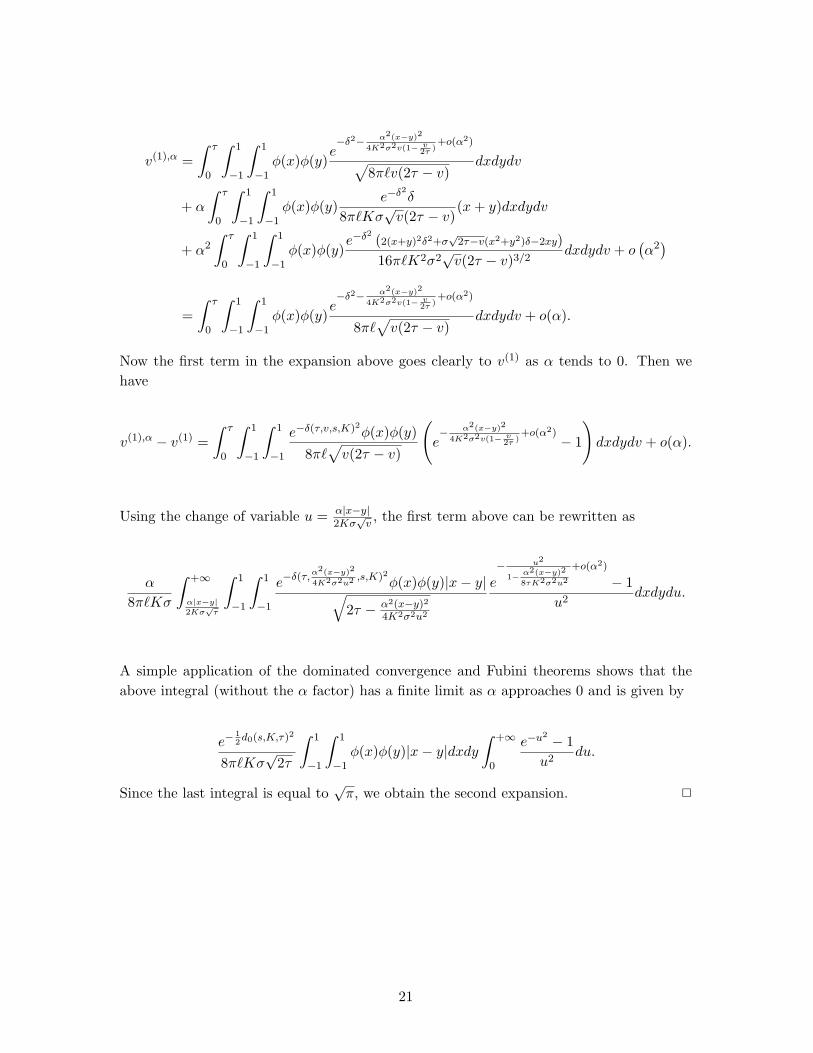
Proof. [Proof of Proposition 6.2] The first result is straightforward and only uses thefact that the function φ is symmetric, which allows us to get rid off the odd terms in theexpansion. For the second one, we directly calculate that

v(1),α =∫ τ

0

∫ 1

−1

∫ 1

−1φ(x)φ(y)

e−δ2− α2(x−y)2

4K2σ2v(1− v2τ )

+o(α2)

8π`√v(2τ − v)

dxdydv

+ α

∫ τ

0

∫ 1

−1

∫ 1

−1φ(x)φ(y)

e−δ2− α2(x−y)2

4K2σ2v(1− v2τ )

+o(α2)δ

8π`Kσ√v(2τ − v)

(x+ y)dxdydv

+ α2

∫ τ

0

∫ 1

−1

∫ 1

−1φ(x)φ(y)

e−δ2− α2(x−y)2

4K2σ2v(1− v2τ )

+o(α2)(2(x+y)2δ2+σ

√2τ−v(x2+y2)δ−2xy)

16π`K2σ2√v(2τ − v)3/2

dxdydv

+ o

α2

∫ τ

0

∫ 1

−1

∫ 1

−1φ(x)φ(y)

e−δ2− α2(x−y)2

4K2σ2v(1− v2τ )

+o(α2)

8π`√v(2τ − v)

dxdydv

,

where we suppressed the arguments of the functions v(1),α and δ for notational simplicity.Note that all the above integrals are well-defined and finite. Then using dominated conver-gence and the fact that φ is symmetric, it is easy to show that

20

v(1),α =∫ τ

0

∫ 1

−1

∫ 1

−1φ(x)φ(y)

e−δ2− α2(x−y)2

4K2σ2v(1− v2τ )

+o(α2)√8π`v(2τ − v)

dxdydv

+ α

∫ τ

0

∫ 1

−1

∫ 1

−1φ(x)φ(y)

e−δ2δ

8π`Kσ√v(2τ − v)

(x+ y)dxdydv

+ α2

∫ τ

0

∫ 1

−1

∫ 1

−1φ(x)φ(y)

e−δ2

(2(x+y)2δ2+σ√

2τ−v(x2+y2)δ−2xy)16π`K2σ2

√v(2τ − v)3/2

dxdydv + o(α2)

=∫ τ

0

∫ 1

−1

∫ 1

−1φ(x)φ(y)

e−δ2− α2(x−y)2

4K2σ2v(1− v2τ )

+o(α2)

8π`√v(2τ − v)

dxdydv + o(α).

Now the first term in the expansion above goes clearly to v(1) as α tends to 0. Then wehave

v(1),α − v(1) =∫ τ

0

∫ 1

−1

∫ 1

−1

e−δ(τ,v,s,K)2φ(x)φ(y)8π`√v(2τ − v)

(e− α2(x−y)2

4K2σ2v(1− v2τ )

+o(α2)− 1

)dxdydv + o(α).

Using the change of variable u = α|x−y|2Kσ

√v, the first term above can be rewritten as

α

8π`Kσ

∫ +∞

α|x−y|2Kσ

√τ

∫ 1

−1

∫ 1

−1

e−δ(τ,α2(x−y)2

4K2σ2u2 ,s,K)2φ(x)φ(y)|x− y|√2τ − α2(x−y)2

4K2σ2u2

e− u2

1− α2(x−y)28τK2σ2u2

+o(α2)

− 1u2

dxdydu.

A simple application of the dominated convergence and Fubini theorems shows that theabove integral (without the α factor) has a finite limit as α approaches 0 and is given by

e−12d0(s,K,τ)2

8π`Kσ√

2τ

∫ 1

−1

∫ 1

−1φ(x)φ(y)|x− y|dxdy

∫ +∞

0

e−u2 − 1u2

du.

Since the last integral is equal to√π, we obtain the second expansion. 2

21