Lambda Calculus - College of Engineering
43
Lambda Calculus 1 / 43
Transcript of Lambda Calculus - College of Engineering
Lambda Calculus
1 / 43
Outline
Introduction and history
Definition of lambda calculusSyntax and operational semanticsMinutia of β-reductionReduction strategies
Programming with lambda calculusChurch encodingsRecursion
De Bruijn indices
Introduction and history 2 / 43
What is the lambda calculus?
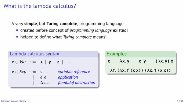
A very simple, but Turing complete, programming language• created before concept of programming language existed!• helped to define what Turing complete means!
Lambda calculus syntax
v ∈ Var ::= x | y | z | . . .
e ∈ Exp ::= v variable reference| e e application| λv. e (lambda) abstraction
Examplesx λx. y x y (λx.y) x
λf.(λx.f (x x)) (λx.f (x x))
Introduction and history 3 / 43
Correspondence to Haskell
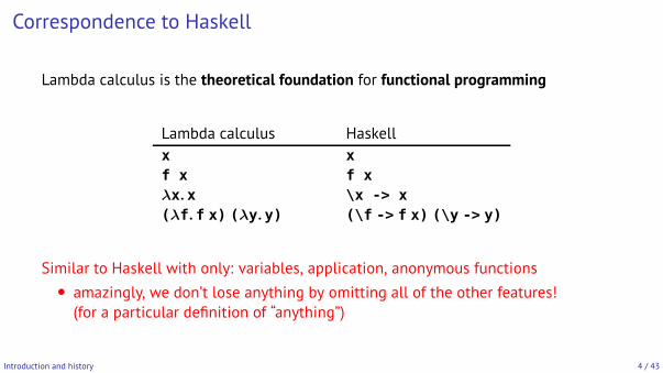
Lambda calculus is the theoretical foundation for functional programming
Lambda calculus Haskellx xf x f xλx.x \x -> x(λf.f x) (λy.y) (\f -> f x) (\y -> y)
Similar to Haskell with only: variables, application, anonymous functions• amazingly, we don’t lose anything by omitting all of the other features!(for a particular definition of “anything”)
Introduction and history 4 / 43
Early history of the lambda calculus
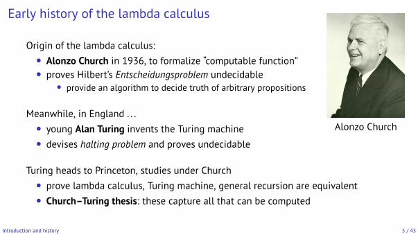
Origin of the lambda calculus:• Alonzo Church in 1936, to formalize “computable function”• proves Hilbert’s Entscheidungsproblem undecidable
• provide an algorithm to decide truth of arbitrary propositions
Meanwhile, in England . . .• young Alan Turing invents the Turing machine• devises halting problem and proves undecidable
Turing heads to Princeton, studies under Church• prove lambda calculus, Turing machine, general recursion are equivalent• Church–Turing thesis: these capture all that can be computed
Introduction and history 5 / 43
Alonzo Church
Why lambda?
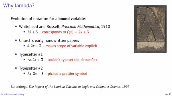
Evolution of notation for a bound variable:
• Whitehead and Russell, Principia Mathematica, 1910• 2x̂ + 3 – corresponds to f (x) = 2x + 3
• Church’s early handwritten papers• x̂. 2x + 3 – makes scope of variable explicit
• Typesetter #1• ^x. 2x + 3 – couldn’t typeset the circumflex!
• Typesetter #2• λx. 2x + 3 – picked a prettier symbol
Barendregt, The Impact of the Lambda Calculus in Logic and Computer Science, 1997
Introduction and history 6 / 43
Impact of the lambda calculus
Turing machine: theoretical foundation for imperative languages• Fortran, Pascal, C, C++, C#, Java, Python, Ruby, JavaScript, . . .
Lambda calculus: theoretical foundation for functional languages• Lisp, ML, Haskell, OCaml, Scheme/Racket, Clojure, F#, Coq, . . .
In programming languages research:• common language of discourse, formal foundation• starting point for new features
• extend syntax, type system, semantics• reveals precise impact and utility of feature
Introduction and history 7 / 43
Outline
Introduction and history
Definition of lambda calculusSyntax and operational semanticsMinutia of β-reductionReduction strategies
Programming with lambda calculusChurch encodingsRecursion
De Bruijn indices
Definition of lambda calculus 8 / 43
Syntax
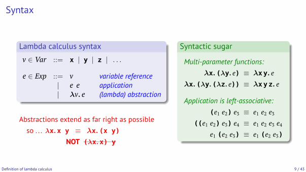
Lambda calculus syntax
v ∈ Var ::= x | y | z | . . .
e ∈ Exp ::= v variable reference| e e application| λv. e (lambda) abstraction
Abstractions extend as far right as possibleso . . . λx.x y ≡ λx. (x y)
NOT (λx.x) y
Syntactic sugar
Multi-parameter functions:λx. (λy. e) ≡ λxy. e
λx. (λy.(λz. e)) ≡ λxyz. e
Application is left-associative:(e1 e2) e3 ≡ e1 e2 e3
((e1 e2) e3) e4 ≡ e1 e2 e3 e4e1 (e2 e3) ≡ e1 (e2 e3)
Definition of lambda calculus 9 / 43
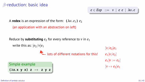
β-reduction: basic idea
A redex is an expression of the form: (λv. e1) e2(an application with an abstraction on left)
Reduce by substituting e2 for every reference to v in e1
write this as: [e2/v]e1
lots of different notations for this!
[v/e2]e1e1[v/e2]
e1[v := e2]
[v 7→ e2]e1Simple example(λx.x y x) z 7→ z y z
Definition of lambda calculus 10 / 43
e ∈ Exp ::= v | e e | λv. e
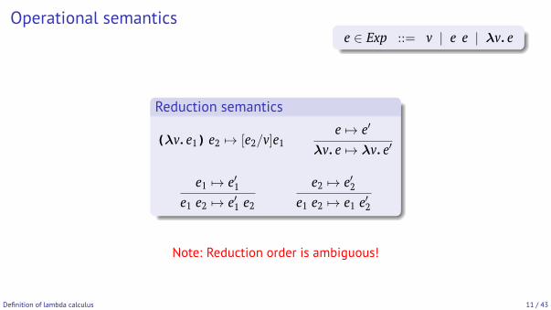
Operational semantics
Reduction semantics
(λv. e1) e2 7→ [e2/v]e1e 7→ e′
λv. e 7→ λv. e′
e1 7→ e′1e1 e2 7→ e′1 e2
e2 7→ e′2e1 e2 7→ e1 e′2
Note: Reduction order is ambiguous!
Definition of lambda calculus 11 / 43
e ∈ Exp ::= v | e e | λv. e
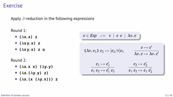
Exercise
Apply β-reduction in the following expressions
Round 1:• (λx.x) z• (λxy.x) z• (λxy.x) z u
Round 2:• (λx.x x) (λy.y)• (λx.(λy.y) z)• (λx.(x (λy.x))) z
Definition of lambda calculus 12 / 43
e ∈ Exp ::= v | e e | λv. e
(λv. e1) e2 7→ [e2/v]e1e 7→ e′
λv. e 7→ λv. e′
e1 7→ e′1e1 e2 7→ e′1 e2
e2 7→ e′2e1 e2 7→ e1 e′2
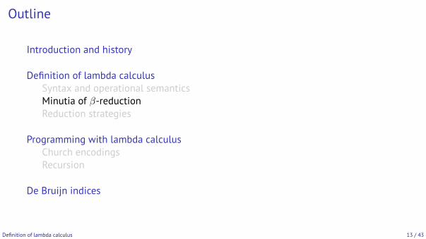
Outline
Introduction and history
Definition of lambda calculusSyntax and operational semanticsMinutia of β-reductionReduction strategies
Programming with lambda calculusChurch encodingsRecursion
De Bruijn indices
Definition of lambda calculus 13 / 43
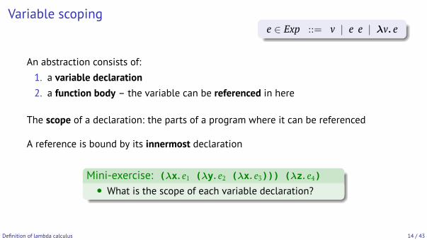
Variable scoping
An abstraction consists of:1. a variable declaration2. a function body – the variable can be referenced in here
The scope of a declaration: the parts of a program where it can be referenced
A reference is bound by its innermost declaration
Mini-exercise: (λx. e1 (λy. e2 (λx. e3))) (λz. e4)• What is the scope of each variable declaration?
Definition of lambda calculus 14 / 43
e ∈ Exp ::= v | e e | λv. e
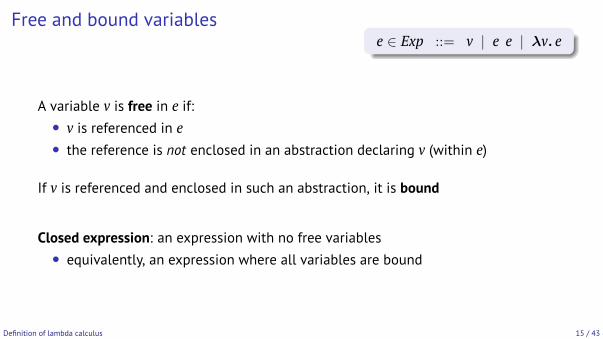
Free and bound variables
A variable v is free in e if:• v is referenced in e• the reference is not enclosed in an abstraction declaring v (within e)
If v is referenced and enclosed in such an abstraction, it is bound
Closed expression: an expression with no free variables• equivalently, an expression where all variables are bound
Definition of lambda calculus 15 / 43
e ∈ Exp ::= v | e e | λv. e
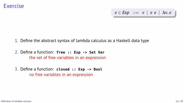
Exercise
1. Define the abstract syntax of lambda calculus as a Haskell data type
2. Define a function: free :: Exp -> Set Varthe set of free variables in an expression
3. Define a function: closed :: Exp -> Boolno free variables in an expression
Definition of lambda calculus 16 / 43
e ∈ Exp ::= v | e e | λv. e
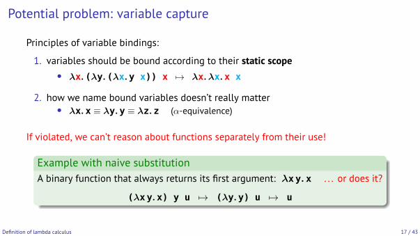
Potential problem: variable capture
Principles of variable bindings:
1. variables should be bound according to their static scope• λx.(λy.(λx.y x)) x 7→ λx. λx.x x
2. how we name bound variables doesn’t really matter• λx.x ≡ λy.y ≡ λz.z (α-equivalence)
If violated, we can’t reason about functions separately from their use!
Example with naive substitutionA binary function that always returns its first argument: λxy. x . . . or does it?
(λxy.x) y u 7→ (λy.y) u 7→ u
Definition of lambda calculus 17 / 43
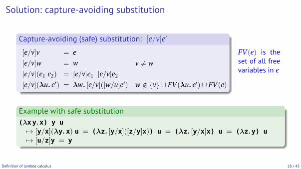
Solution: capture-avoiding substitution
Capture-avoiding (safe) substitution: [e/v]e′
[e/v]v = e[e/v]w = w v 6= w[e/v](e1 e2) = [e/v]e1 [e/v]e2[e/v](λu. e′) = λw. [e/v]([w/u]e′) w /∈ {v} ∪ FV(λu. e′) ∪ FV(e)
FV(e) is theset of all freevariables in e
Example with safe substitution(λxy.x) y u7→ [y/x](λy. x) u = (λz. [y/x]([z/y]x)) u = (λz. [y/x]x) u = (λz.y) u7→ [u/z]y = y
Definition of lambda calculus 18 / 43
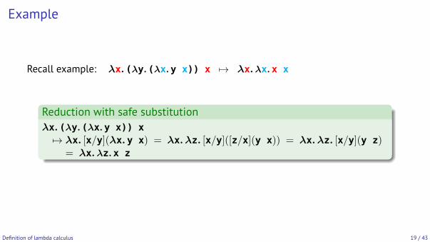
Example
Recall example: λx. (λy.(λx.y x)) x 7→ λx.λx.x x
Reduction with safe substitutionλx. (λy.(λx.y x)) x7→ λx. [x/y](λx. y x) = λx. λz. [x/y]([z/x](y x)) = λx. λz. [x/y](y z)
= λx.λz.x z
Definition of lambda calculus 19 / 43
Outline
Introduction and history
Definition of lambda calculusSyntax and operational semanticsMinutia of β-reductionReduction strategies
Programming with lambda calculusChurch encodingsRecursion
De Bruijn indices
Definition of lambda calculus 20 / 43
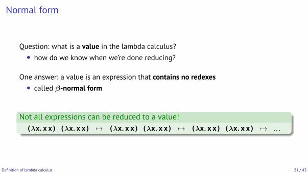
Normal form
Question: what is a value in the lambda calculus?• how do we know when we’re done reducing?
One answer: a value is an expression that contains no redexes• called β-normal form
Not all expressions can be reduced to a value!(λx.xx) (λx.xx) 7→ (λx.xx) (λx.xx) 7→ (λx.xx) (λx.xx) 7→ . . .
Definition of lambda calculus 21 / 43
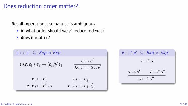
Does reduction order matter?
Recall: operational semantics is ambiguous• in what order should we β-reduce redexes?• does it matter?
e 7→ e′ ⊆ Exp× Exp
(λv. e1) e2 7→ [e2/v]e1e 7→ e′
λv. e 7→ λv. e′
e1 7→ e′1e1 e2 7→ e′1 e2
e2 7→ e′2e1 e2 7→ e1 e′2
e 7→∗ e′ ⊆ Exp× Exps 7→∗ s
s 7→ s′ s′ 7→∗ s′′
s 7→∗ s′′
Definition of lambda calculus 22 / 43
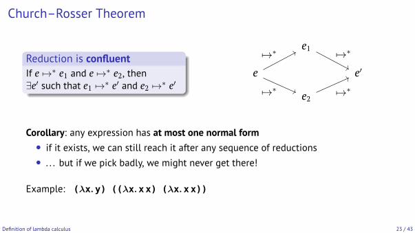
Church–Rosser Theorem
Reduction is confluentIf e 7→∗ e1 and e 7→∗ e2, then∃e′ such that e1 7→∗ e′ and e2 7→∗ e′
e1
e e′
e2
7→∗7→∗
7→∗ 7→∗
Corollary: any expression has at most one normal form• if it exists, we can still reach it after any sequence of reductions• . . . but if we pick badly, we might never get there!
Example: (λx.y) ((λx.xx) (λx.xx))
Definition of lambda calculus 23 / 43
Reduction strategies
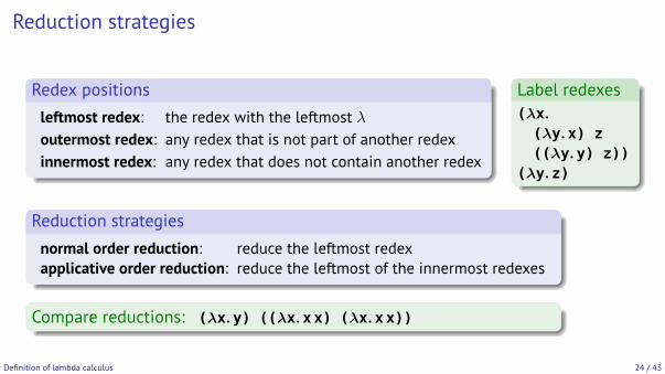
Redex positionsleftmost redex: the redex with the leftmost λoutermost redex: any redex that is not part of another redexinnermost redex: any redex that does not contain another redex
Label redexes(λx.(λy.x) z((λy.y) z))
(λy.z)
Reduction strategiesnormal order reduction: reduce the leftmost redexapplicative order reduction: reduce the leftmost of the innermost redexes
Compare reductions: (λx.y) ((λx.xx) (λx.xx))
Definition of lambda calculus 24 / 43
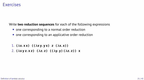
Exercises
Write two reduction sequences for each of the following expressions• one corresponding to a normal order reduction• one corresponding to an applicative order reduction
1. (λx.xx) ((λxy.yx) z (λx.x))2. (λxyz.xz) (λz.z) ((λy.y)(λz.z)) x
Definition of lambda calculus 25 / 43
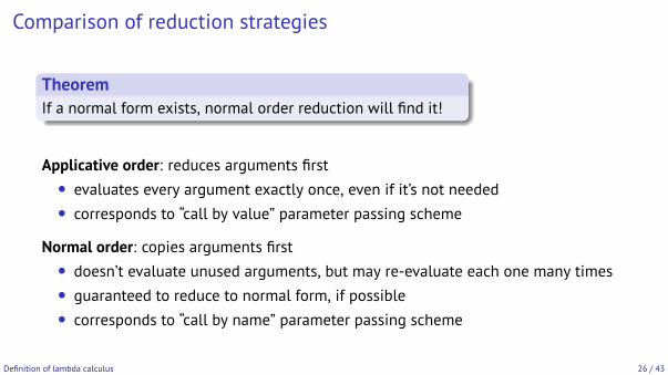
Comparison of reduction strategies
TheoremIf a normal form exists, normal order reduction will find it!
Applicative order: reduces arguments first• evaluates every argument exactly once, even if it’s not needed• corresponds to “call by value” parameter passing scheme
Normal order: copies arguments first• doesn’t evaluate unused arguments, but may re-evaluate each one many times• guaranteed to reduce to normal form, if possible• corresponds to “call by name” parameter passing scheme
Definition of lambda calculus 26 / 43
Brief notes on lazy evaluation
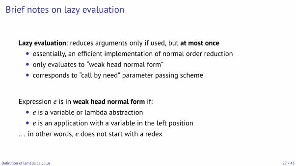
Lazy evaluation: reduces arguments only if used, but at most once• essentially, an efficient implementation of normal order reduction• only evaluates to “weak head normal form”• corresponds to “call by need” parameter passing scheme
Expression e is in weak head normal form if:• e is a variable or lambda abstraction• e is an application with a variable in the left position
. . . in other words, e does not start with a redex
Definition of lambda calculus 27 / 43
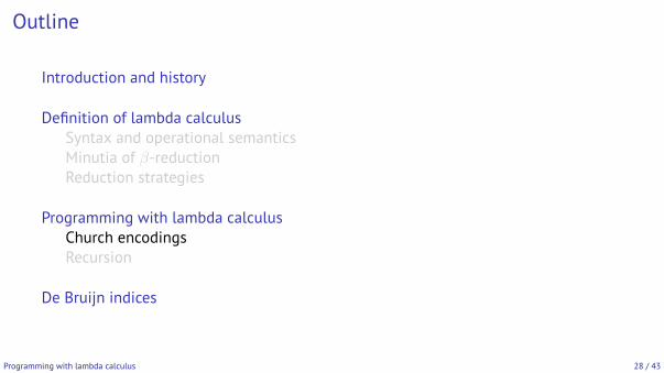
Outline
Introduction and history
Definition of lambda calculusSyntax and operational semanticsMinutia of β-reductionReduction strategies
Programming with lambda calculusChurch encodingsRecursion
De Bruijn indices
Programming with lambda calculus 28 / 43
Church Booleans
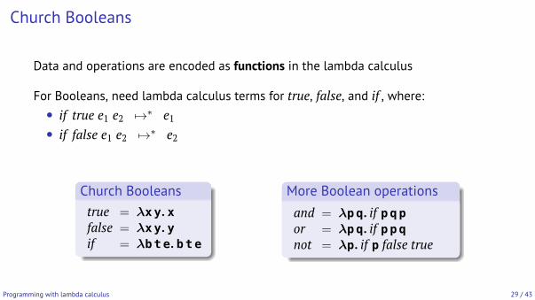
Data and operations are encoded as functions in the lambda calculus
For Booleans, need lambda calculus terms for true, false, and if , where:• if true e1 e2 7→∗ e1• if false e1 e2 7→∗ e2
Church Booleanstrue = λxy. xfalse = λxy. yif = λbte. bte
More Boolean operationsand = λpq. if pqpor = λpq. if ppqnot = λp. if p false true
Programming with lambda calculus 29 / 43
Church numerals
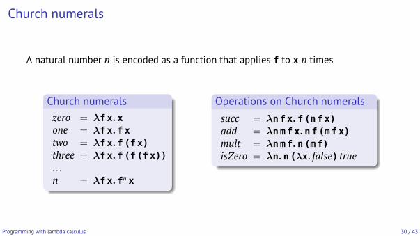
A natural number n is encoded as a function that applies f to x n times
Church numeralszero = λfx. xone = λfx. fxtwo = λfx. f(fx)three = λfx. f(f(fx)). . .n = λfx. fn x
Operations on Church numeralssucc = λnfx. f(nfx)add = λnmfx. nf(mfx)mult = λnmf. n(mf)isZero = λn. n(λx. false) true
Programming with lambda calculus 30 / 43
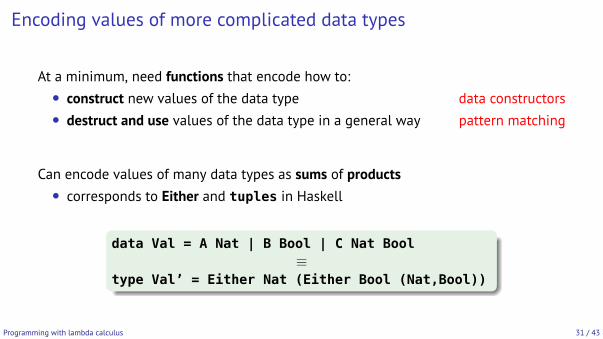
Encoding values of more complicated data types
At a minimum, need functions that encode how to:• construct new values of the data type data constructors• destruct and use values of the data type in a general way pattern matching
Can encode values of many data types as sums of products• corresponds to Either and tuples in Haskell
data Val = A Nat | B Bool | C Nat Bool≡
type Val’ = Either Nat (Either Bool (Nat,Bool))
Programming with lambda calculus 31 / 43
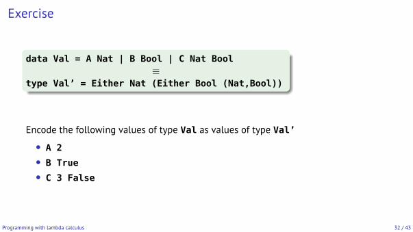
Exercise
data Val = A Nat | B Bool | C Nat Bool≡
type Val’ = Either Nat (Either Bool (Nat,Bool))
Encode the following values of type Val as values of type Val’
• A 2• B True• C 3 False
Programming with lambda calculus 32 / 43
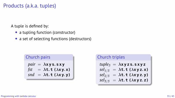
Products (a.k.a. tuples)
A tuple is defined by:• a tupling function (constructor)• a set of selecting functions (destructors)
Church pairspair = λxys. sxyfst = λt. t (λxy.x)snd = λt. t (λxy.y)
Church triplestuple3 = λxyzs. sxyzsel1/3 = λt. t (λxyz.x)sel2/3 = λt. t (λxyz.y)sel3/3 = λt. t (λxyz.z)
Programming with lambda calculus 33 / 43
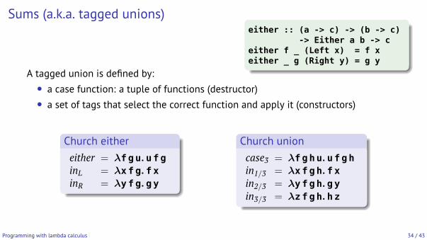
Sums (a.k.a. tagged unions)
A tagged union is defined by:• a case function: a tuple of functions (destructor)• a set of tags that select the correct function and apply it (constructors)
Church eithereither = λfgu. ufginL = λxfg. fxinR = λyfg. gy
Church unioncase3 = λfghu. ufghin1/3 = λxfgh. fxin2/3 = λyfgh. gyin3/3 = λzfgh. hz
Programming with lambda calculus 34 / 43
either :: (a -> c) -> (b -> c)-> Either a b -> c
either f _ (Left x) = f xeither _ g (Right y) = g y
Exercise
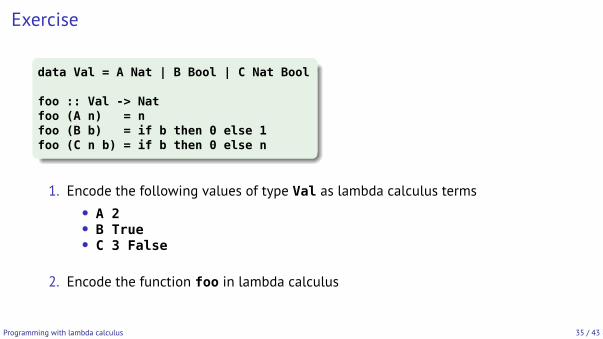
data Val = A Nat | B Bool | C Nat Bool
foo :: Val -> Natfoo (A n) = nfoo (B b) = if b then 0 else 1foo (C n b) = if b then 0 else n
1. Encode the following values of type Val as lambda calculus terms• A 2• B True• C 3 False
2. Encode the function foo in lambda calculus
Programming with lambda calculus 35 / 43
Outline
Introduction and history
Definition of lambda calculusSyntax and operational semanticsMinutia of β-reductionReduction strategies
Programming with lambda calculusChurch encodingsRecursion
De Bruijn indices
Programming with lambda calculus 36 / 43
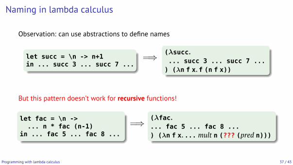
Naming in lambda calculus
Observation: can use abstractions to define names
let succ = \n -> n+1in ... succ 3 ... succ 7 ...
=⇒ (λsucc.... succ 3 ... succ 7 ...
) (λn f x.f (n f x))
But this pattern doesn’t work for recursive functions!
let fac = \n ->... n * fac (n-1)
in ... fac 5 ... fac 8 ...=⇒ (λfac.
... fac 5 ... fac 8 ...) (λn f x.... mult n (??? (pred n)))
Programming with lambda calculus 37 / 43
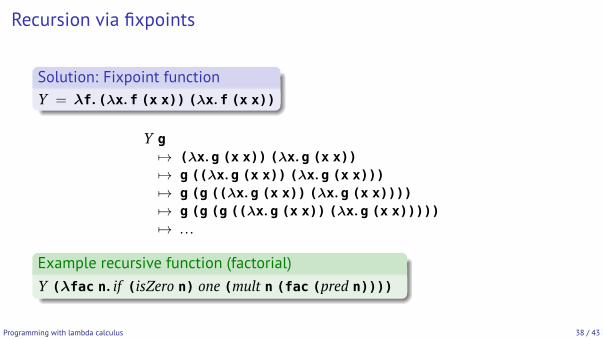
Recursion via fixpoints
Solution: Fixpoint functionY = λf. (λx.f (x x)) (λx.f (x x))
Y g7→ (λx.g (x x)) (λx.g (x x))7→ g ((λx.g (x x)) (λx.g (x x)))7→ g (g ((λx.g (x x)) (λx.g (x x))))7→ g (g (g ((λx.g (x x)) (λx.g (x x)))))7→ . . .
Example recursive function (factorial)Y (λfac n. if (isZero n) one (mult n (fac (pred n))))
Programming with lambda calculus 38 / 43
Outline
Introduction and history
Definition of lambda calculusSyntax and operational semanticsMinutia of β-reductionReduction strategies
Programming with lambda calculusChurch encodingsRecursion
De Bruijn indices
De Bruijn indices 39 / 43
The role of names in lambda calculus
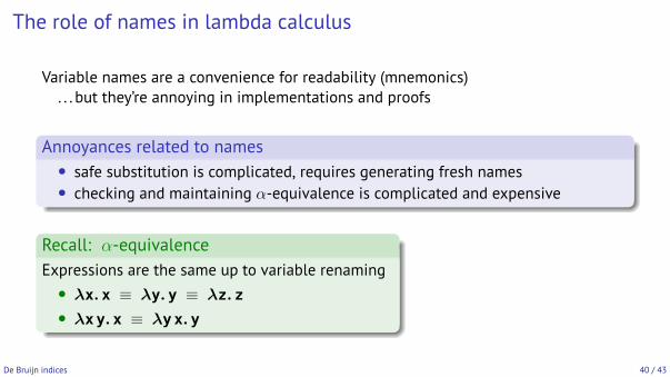
Variable names are a convenience for readability (mnemonics). . . but they’re annoying in implementations and proofs
Annoyances related to names• safe substitution is complicated, requires generating fresh names• checking and maintaining α-equivalence is complicated and expensive
Recall: α-equivalenceExpressions are the same up to variable renaming• λx. x ≡ λy. y ≡ λz. z• λxy. x ≡ λyx. y
De Bruijn indices 40 / 43
A nameless representation of lambda calculus
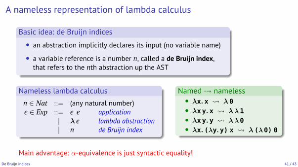
Basic idea: de Bruijn indices• an abstraction implicitly declares its input (no variable name)
• a variable reference is a number n, called a de Bruijn index,that refers to the nth abstraction up the AST
Nameless lambda calculus
n ∈ Nat ::= (any natural number)e ∈ Exp ::= e e application
| λ e lambda abstraction| n de Bruijn index
Named nameless• λx. x λ 0• λxy. x λλ1• λxy. y λλ0• λx. (λy.y) x λ (λ0) 0
Main advantage: α-equivalence is just syntactic equality!De Bruijn indices 41 / 43
Deciphering de Bruijn indices
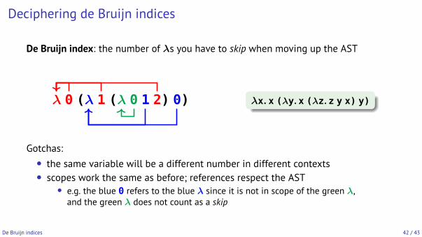
De Bruijn index: the number of λs you have to skip when moving up the AST
λ 0 (λ 1 (λ 0 1 2) 0) λx. x (λy.x (λz.z y x) y)
Gotchas:• the same variable will be a different number in different contexts• scopes work the same as before; references respect the AST
• e.g. the blue 0 refers to the blue λ since it is not in scope of the green λ,and the green λ does not count as a skip
De Bruijn indices 42 / 43
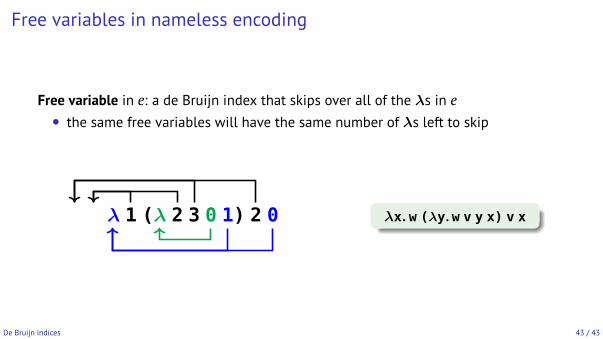
Free variables in nameless encoding
Free variable in e: a de Bruijn index that skips over all of the λs in e• the same free variables will have the same number of λs left to skip
λ 1 (λ 2 3 0 1) 2 0 λx. w (λy.w v y x) v x
De Bruijn indices 43 / 43


![Lambda Calculus - SJTUyuxi/teaching/lectures/Lambda Calculus.pdf · Lambda Calculus Alonzo Church [14Jun.1903-11Aug.1995] invented the -Calculus with a foundational motivation [1932].](https://static.fdocument.org/doc/165x107/5fb2b5193e095c5efe6ac4f7/lambda-calculus-sjtu-yuxiteachinglectureslambda-calculuspdf-lambda-calculus.jpg)
![COMP4630: [fg]structure-Calculus - 1. BasicsIntroduction Lambda Calculus Terms Alpha Equivalence Substitution Dynamics Beta Reduction Eta Reduction Normal Forms Evaluation Strategies](https://static.fdocument.org/doc/165x107/5fd846ab2233da093f0d9793/comp4630-fgstructure-calculus-1-basics-introduction-lambda-calculus-terms.jpg)