LAB Exercise #9 Strain Analysis - University of California...
6
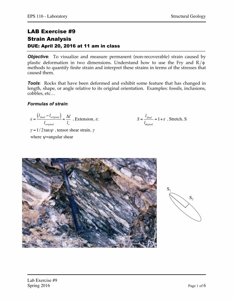
EPS 116 - Laboratory Structural Geology Lab Exercise #9 Spring 2016 Page 1 of 6 LAB Exercise #9 Strain Analysis DUE: April 20, 2016 at 11 am in class Objective: To visualize and measure permanent (non-recoverable) strain caused by plastic deformation in two dimensions. Understand how to use the Fry and Rf/φ methods to quantify finite strain and interpret these strains in terms of the stresses that caused them. Tools: Rocks that have been deformed and exhibit some feature that has changed in length, shape, or angle relative to its original orientation. Examples: fossils, inclusions, cobbles, etc… Formulas of strain: ε = l final − l original ( ) l original = Δl l o , Extension, ε; S = l final l original = 1 + ε , Stretch, S γ = 1 / 2 tan ψ , tensor shear strain, γ where ψ =angular shear S 2 S 1
Transcript of LAB Exercise #9 Strain Analysis - University of California...
EPS 116 - Laboratory Structural Geology
Lab Exercise #9 Spring 2016 Page 1 of 6
LAB Exercise #9
Strain Analysis DUE: April 20, 2016 at 11 am in class Objective: To visualize and measure permanent (non-recoverable) strain caused by plastic deformation in two dimensions. Understand how to use the Fry and Rf/φ methods to quantify finite strain and interpret these strains in terms of the stresses that caused them. Tools: Rocks that have been deformed and exhibit some feature that has changed in length, shape, or angle relative to its original orientation. Examples: fossils, inclusions, cobbles, etc… Formulas of strain:
ε =l final − loriginal( )loriginal
=Δllo
, Extension, ε; S =l finalloriginal
=1+ε , Stretch, S
γ =1/ 2 tanψ , tensor shear strain, γwhere ψ=angular shear
S2
S1
EPS 116 - Laboratory Structural Geology
Lab Exercise #9 Spring 2016 Page 2 of 6
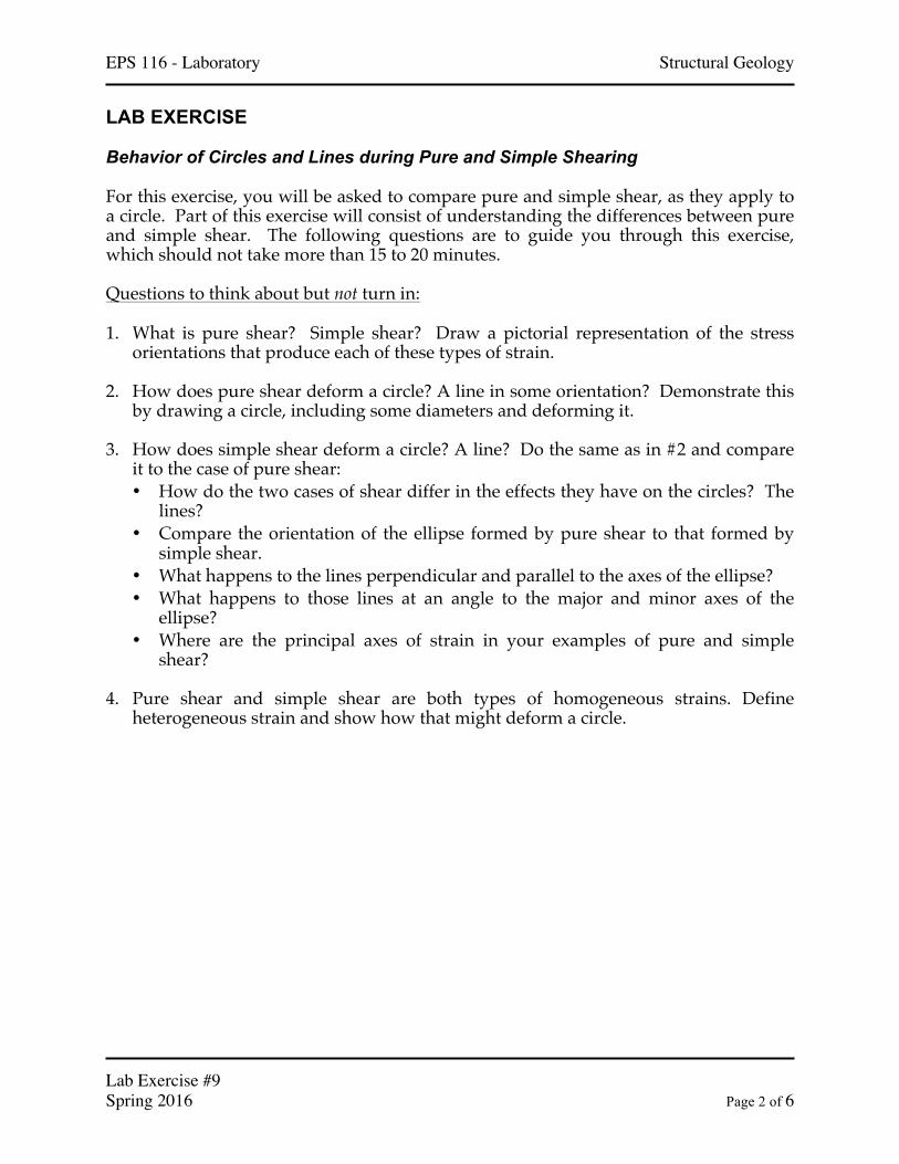
LAB EXERCISE Behavior of Circles and Lines during Pure and Simple Shearing For this exercise, you will be asked to compare pure and simple shear, as they apply to a circle. Part of this exercise will consist of understanding the differences between pure and simple shear. The following questions are to guide you through this exercise, which should not take more than 15 to 20 minutes. Questions to think about but not turn in: 1. What is pure shear? Simple shear? Draw a pictorial representation of the stress
orientations that produce each of these types of strain.
2. How does pure shear deform a circle? A line in some orientation? Demonstrate this by drawing a circle, including some diameters and deforming it.
3. How does simple shear deform a circle? A line? Do the same as in #2 and compare it to the case of pure shear: • How do the two cases of shear differ in the effects they have on the circles? The
lines? • Compare the orientation of the ellipse formed by pure shear to that formed by
simple shear. • What happens to the lines perpendicular and parallel to the axes of the ellipse? • What happens to those lines at an angle to the major and minor axes of the
ellipse? • Where are the principal axes of strain in your examples of pure and simple
shear?
4. Pure shear and simple shear are both types of homogeneous strains. Define heterogeneous strain and show how that might deform a circle.
EPS 116 - Laboratory Structural Geology
Lab Exercise #9 Spring 2016 Page 3 of 6
The Fry Method Fry, N. (1979) Random point distributions and strain measurements in rocks, Tectonophysics 60: 89-105. Summary of method presented in Twiss & Moores p. 453. The Fry method is a graphical technique for determining the strain ellipse ! Assume an initial uniform point distribution (isotropic). ! After deformation, the point distribution is non-uniform ! Where extension has occurred, distances between points increase; where contraction
has occurred, distances decrease. ! The maximum distance between points occurs parallel to principal stretch direction,
S1, while minimum distance occurs parallel to S2. The Method 1. Mark the center of each object on a tracing paper overlay (Centers Sheet) 2. Copy the dots onto a second overlay and choose a central reference point (Reference
Sheet). You should now have two identical pieces of tracing paper with a bunch of dots.
3. Place the Reference Sheet on top of the Centers sheet. 4. Line up the reference point with another point on the Centers Sheet 5. Trace all the dots from the Centers Sheet onto the Reference Sheet. They should
show up in different locations because you’ve moved the Reference Sheet. 6. Repeat the process with the Reference point lining up with every other point. Your
final product will have a lot of points (~ n2-n points) 7. If all goes as planned you should clearly see the strain ellipse around the reference
point, which shows up as either an elliptical area devoid of points or an elliptical area of concentrated points.
8. Draw in your interpretation of the strain ellipse size and orientation.
Strengths ! Quick and easy ! Can be used on rocks that have pressure solution along grain boundaries, i.e.
rocks in which some original material may have been lost ! Applies to sand grains in sandstone, ooids in limestone, and pebbles in a
conglomerate
Weaknesses ! Requires lots of points (at least 25 for more precise answers) ! Estimates of ellipticity can be subjective and, hence, inaccurate ! Cannot be used if particles being analyzed had some preferred axial direction
prior to deformation
EPS 116 - Laboratory Structural Geology
Lab Exercise #9 Spring 2016 Page 4 of 6
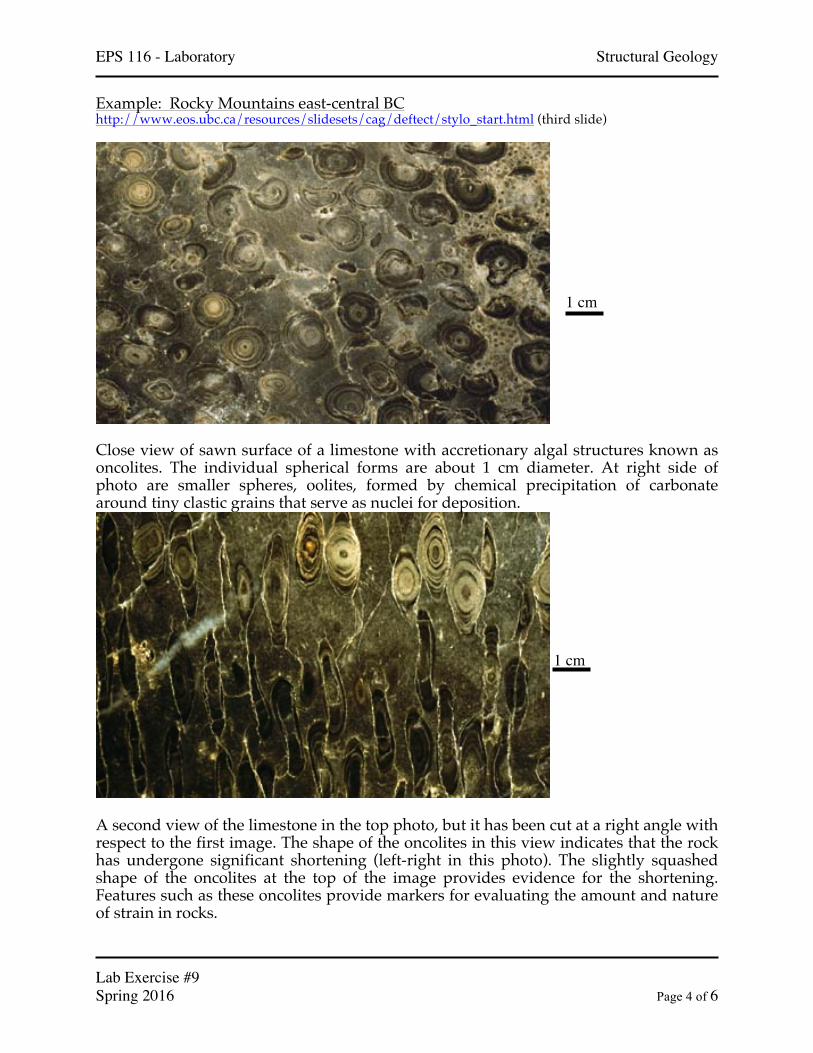
Example: Rocky Mountains east-central BC http://www.eos.ubc.ca/resources/slidesets/cag/deftect/stylo_start.html (third slide)
Close view of sawn surface of a limestone with accretionary algal structures known as oncolites. The individual spherical forms are about 1 cm diameter. At right side of photo are smaller spheres, oolites, formed by chemical precipitation of carbonate around tiny clastic grains that serve as nuclei for deposition.
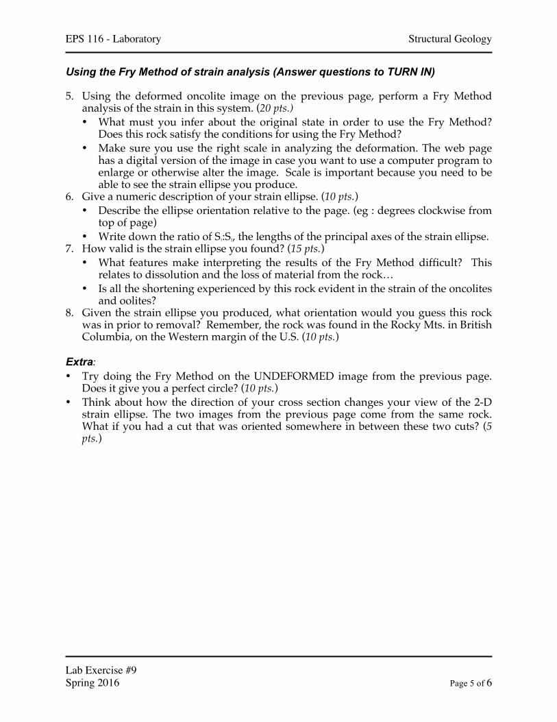
A second view of the limestone in the top photo, but it has been cut at a right angle with respect to the first image. The shape of the oncolites in this view indicates that the rock has undergone significant shortening (left-right in this photo). The slightly squashed shape of the oncolites at the top of the image provides evidence for the shortening. Features such as these oncolites provide markers for evaluating the amount and nature of strain in rocks.
1 cm
1 cm
EPS 116 - Laboratory Structural Geology
Lab Exercise #9 Spring 2016 Page 5 of 6
Using the Fry Method of strain analysis (Answer questions to TURN IN) 5. Using the deformed oncolite image on the previous page, perform a Fry Method
analysis of the strain in this system. (20 pts.) • What must you infer about the original state in order to use the Fry Method?
Does this rock satisfy the conditions for using the Fry Method? • Make sure you use the right scale in analyzing the deformation. The web page
has a digital version of the image in case you want to use a computer program to enlarge or otherwise alter the image. Scale is important because you need to be able to see the strain ellipse you produce.
6. Give a numeric description of your strain ellipse. (10 pts.) • Describe the ellipse orientation relative to the page. (eg : degrees clockwise from
top of page) • Write down the ratio of S1:S2, the lengths of the principal axes of the strain ellipse.
7. How valid is the strain ellipse you found? (15 pts.) • What features make interpreting the results of the Fry Method difficult? This
relates to dissolution and the loss of material from the rock… • Is all the shortening experienced by this rock evident in the strain of the oncolites
and oolites? 8. Given the strain ellipse you produced, what orientation would you guess this rock
was in prior to removal? Remember, the rock was found in the Rocky Mts. in British Columbia, on the Western margin of the U.S. (10 pts.)
Extra: • Try doing the Fry Method on the UNDEFORMED image from the previous page.
Does it give you a perfect circle? (10 pts.) • Think about how the direction of your cross section changes your view of the 2-D
strain ellipse. The two images from the previous page come from the same rock. What if you had a cut that was oriented somewhere in between these two cuts? (5 pts.)
EPS 116 - Laboratory Structural Geology
Lab Exercise #9 Spring 2016 Page 6 of 6
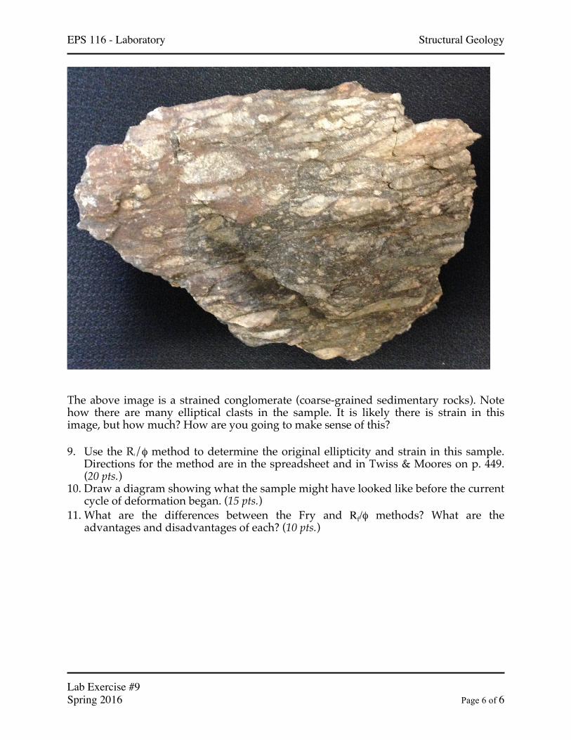
The above image is a strained conglomerate (coarse-grained sedimentary rocks). Note how there are many elliptical clasts in the sample. It is likely there is strain in this image, but how much? How are you going to make sense of this? 9. Use the Rf/φ method to determine the original ellipticity and strain in this sample.
Directions for the method are in the spreadsheet and in Twiss & Moores on p. 449. (20 pts.)
10. Draw a diagram showing what the sample might have looked like before the current cycle of deformation began. (15 pts.)
11. What are the differences between the Fry and Rf/φ methods? What are the advantages and disadvantages of each? (10 pts.)


![Geology · Geology Forthescientificjournal,seeGeology(journal). Geology(fromtheAncientGreekγῆ,gē,i.e.“earth”and-λoγία,-logia,i.e.“studyof,discourse”[1][2 ...](https://static.fdocument.org/doc/165x107/5f512a8dc36d4d05a271efd1/geology-geology-forthescientiicjournalseegeologyjournal-geologyfromtheancientgreekgieaoeearthaand-o-logiaieaoestudyofdiscoursea12.jpg)