L18: CAPM 1

Lecture 18: Testing CAPM

• The following topics will be covered:• Time Series Tests

– Sharpe (1964)/Litner (1965) version

– Black (1972) version

• Cross Sectional Tests– Fama-MacBeth (1973) Approach

L18: CAPM 2

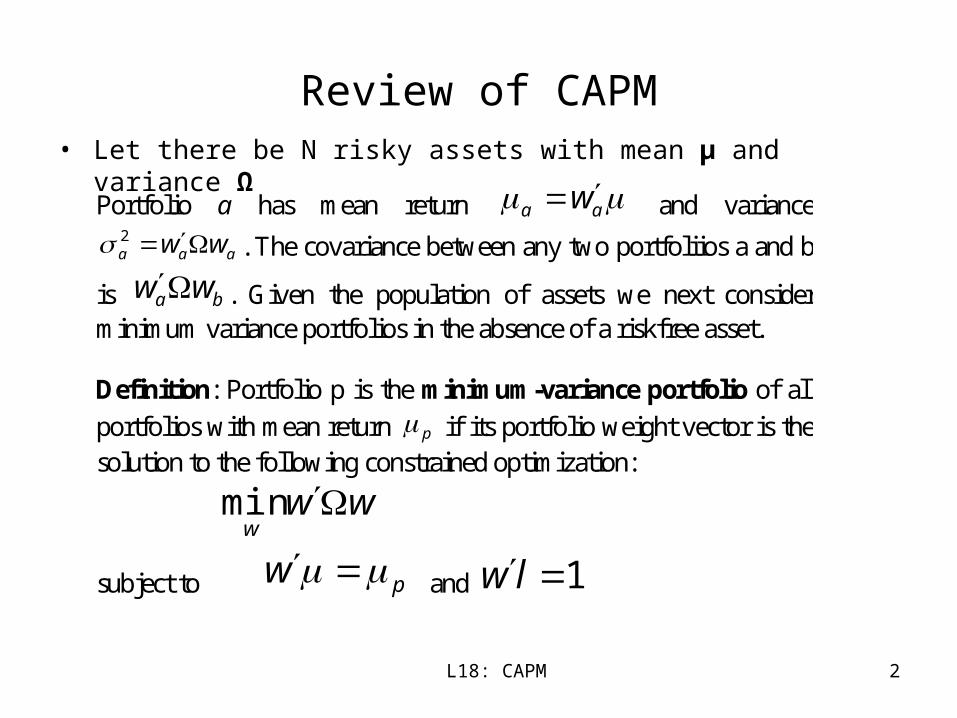
Review of CAPM• Let there be N risky assets with mean µ and variance Ω

Portfolio a has mean return aa w and variance

aaa ww 2 . The covariance between any two portfoliios a and b

is ba ww . Given the population of assets we next consider minimum variance portfolios in the absence of a riskfree asset. Definition: Portfolio p is the minimum-variance portfolio of all

portfolios with mean return p if its portfolio weight vector is the solution to the following constrained optimization:

www

min

subject to pw and 1lw

L18: CAPM 3

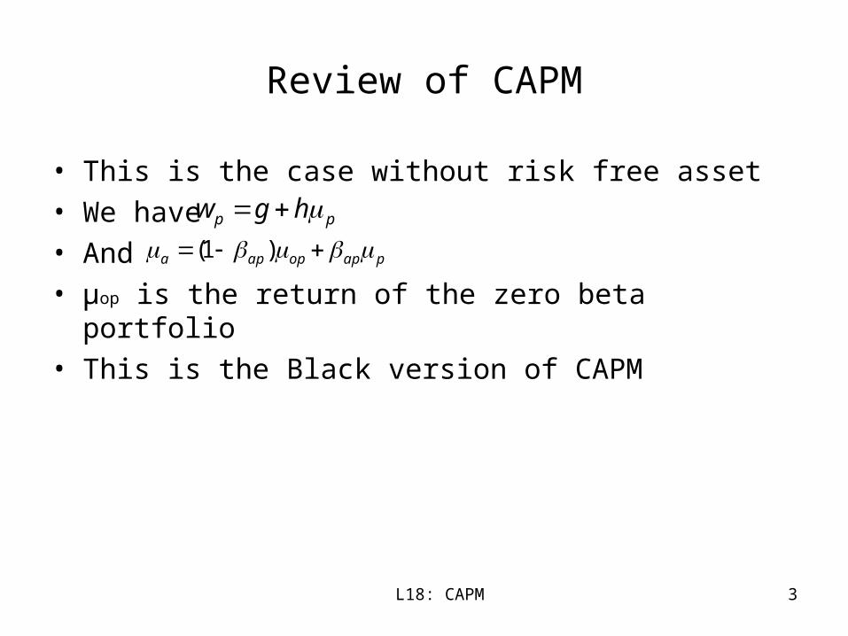
Review of CAPM

• This is the case without risk free asset

• We have

• And

• µop is the return of the zero beta portfolio

• This is the Black version of CAPM

pp hgw

papopapa )1(

L18: CAPM 4

Review of CAPM

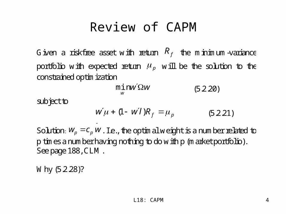
Given a riskfree asset with return fR the minimum-variance

portfolio with expected return p will be the solution to the constrained optimization

www

min (5.2.20)

subject to

pfRlww )1( (5.2.21)

Solution:

wcw pp . I.e., the optimal weight is a number related to p times a number having nothing to do with p (market portfolio). See page 188, CLM. Why (5.2.28)?

L18: CAPM 5

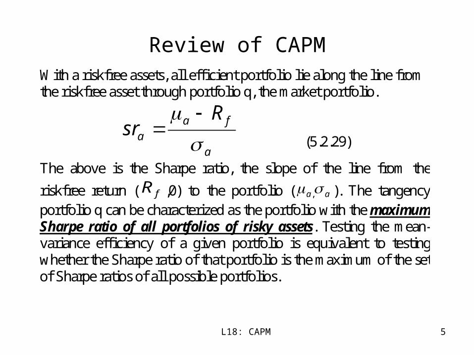
Review of CAPMWith a riskfree assets, all efficient portfolio lie along the line from the riskfree asset through portfolio q, the market portfolio.

a

faa

Rsr

(5.2.29)

The above is the Sharpe ratio, the slope of the line from the

riskfree return ( fR ,0) to the portfolio ( aa , ). The tangency portfolio q can be characterized as the portfolio with the maximum Sharpe ratio of all portfolios of risky assets. Testing the mean-variance efficiency of a given portfolio is equivalent to testing whether the Sharpe ratio of that portfolio is the maximum of the set of Sharpe ratios of all possible portfolios.

L18: CAPM 6

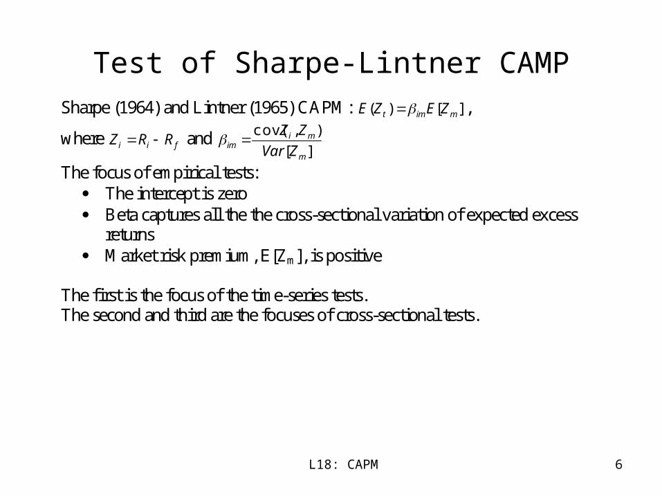
Test of Sharpe-Lintner CAMPSharpe (1964) and Lintner (1965) CAPM: ][)( mimt ZEZE ,

where fii RRZ and ][

),cov(

m

miim ZVar

ZZ

The focus of empirical tests: The intercept is zero Beta captures all the the cross-sectional variation of expected excess

returns Market risk premium, E[Zm], is positive

The first is the focus of the time-series tests. The second and third are the focuses of cross-sectional tests.

L18: CAPM 7

Time-Series Tests: Maximum Likelihood Approach

• There are N assets and hence, N equations.

• For each equation, we can run OLS and obtain estimates of i and i, I = 1,…,N.

• We could also estimate the equations jointly.

• Is there any advantage to doing this, that is, run the “seemingly unrelated” regression on the system?

• As it turns out, joint estimation is useless if we only need estimates for ’s and ’s.

• However, for our joint test, it’s not useless. We need the covariance matrix for our joint test.

L18: CAPM 8

The Likelihood Function

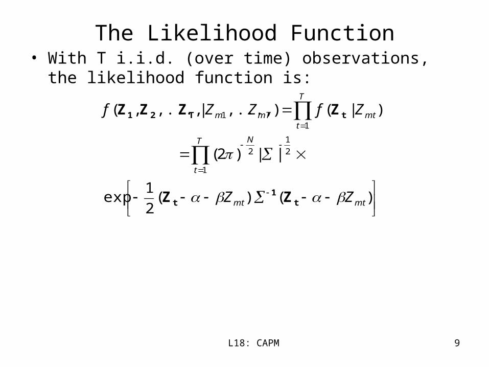
• We will assume that the distribution for excess returns are jointly normal. This is critical for the maximum likelihood approach. However, if we use Quasi ML, or GMM, we do not need normality assumption.

• Given joint normality of excess returns, the likelihood function for the cross-section of excess returns in a single period is:

)()'(2

1exp||)2()|( 2

1

2mtmt

N

mt ZZZf t1

tt ZZZ

L18: CAPM 9

The Likelihood Function• With T i.i.d. (over time) observations, the likelihood function

is:

)()'(2

1exp

||)2(

)|(),...,|,...,,(

1

2

1

2

11

mtmt

T

t

N

T

tmtmTm

ZZ

ZfZZf

t1

t

tT21

ZZ

ZZZZ

L18: CAPM 10

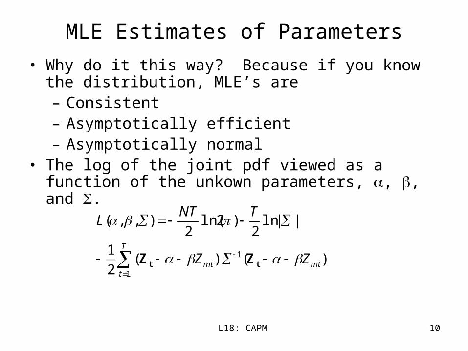
MLE Estimates of Parameters

• Why do it this way? Because if you know the distribution, MLE’s are – Consistent– Asymptotically efficient– Asymptotically normal

• The log of the joint pdf viewed as a function of the unkown parameters, , , and .

)()'(2

1

||ln2

)2ln(2

),,(

1

1mt

T

tmt ZZ

TNTL

tt ZZ

L18: CAPM 11

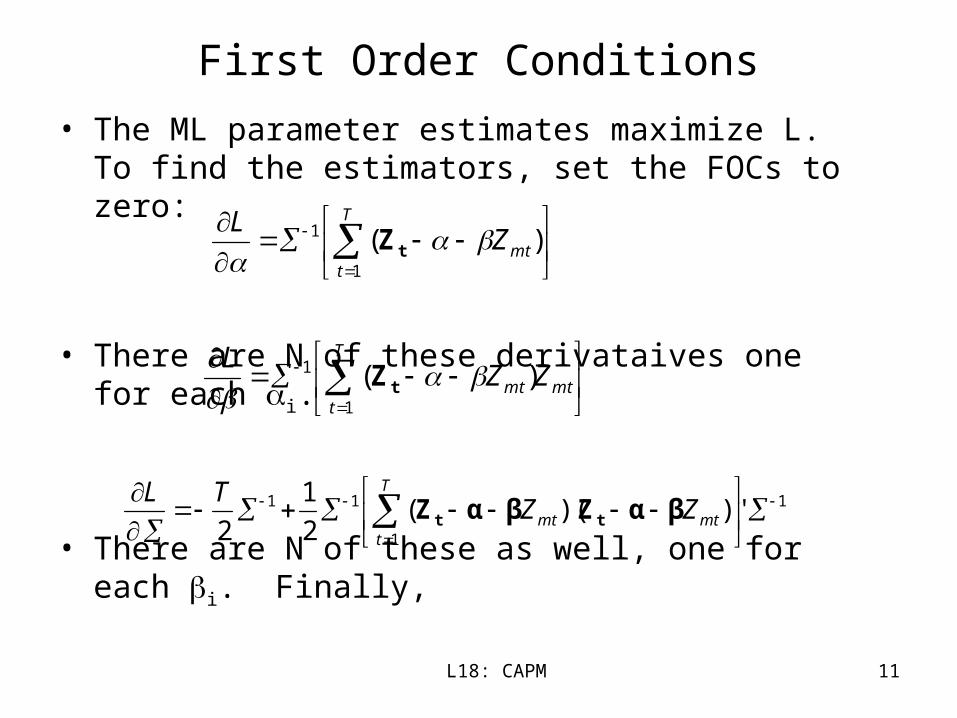
First Order Conditions

• The ML parameter estimates maximize L. To find the estimators, set the FOCs to zero:

• There are N of these derivataives one for each i.

• There are N of these as well, one for each i. Finally,

T

tmtZ

L

1

1 )( tZ

mt

T

tmt ZZ

L

1

1 )( tZ

1

1

11 )')((2

1

2

T

tmtmt ZZ

TLβαZβαZ tt

L18: CAPM 12

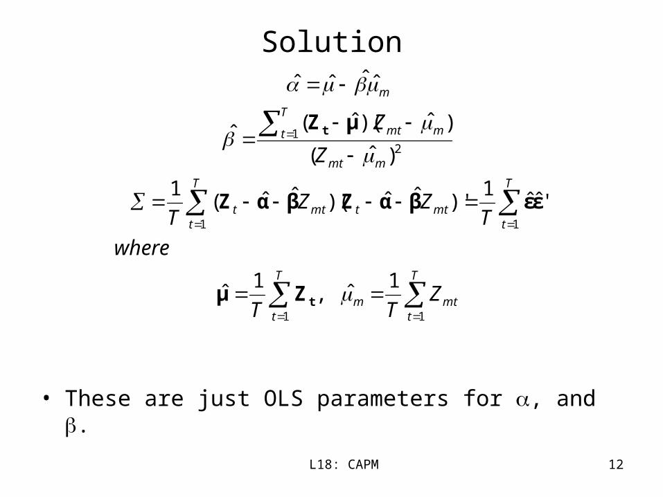
Solution

• These are just OLS parameters for , and .

T

tmtm

T

t

T

t

T

tmttmtt

mmt

T

t mmt

m

ZTT

where

TZZ

T

Z

Z

11

11

21

1ˆ,

1ˆ

'ˆˆ1

)'ˆˆ)(ˆˆ(1

)ˆ(

)ˆ)(ˆ(ˆ

ˆˆˆˆ

t

t

Zμ

εεβαZβαZ

μZ

L18: CAPM 13

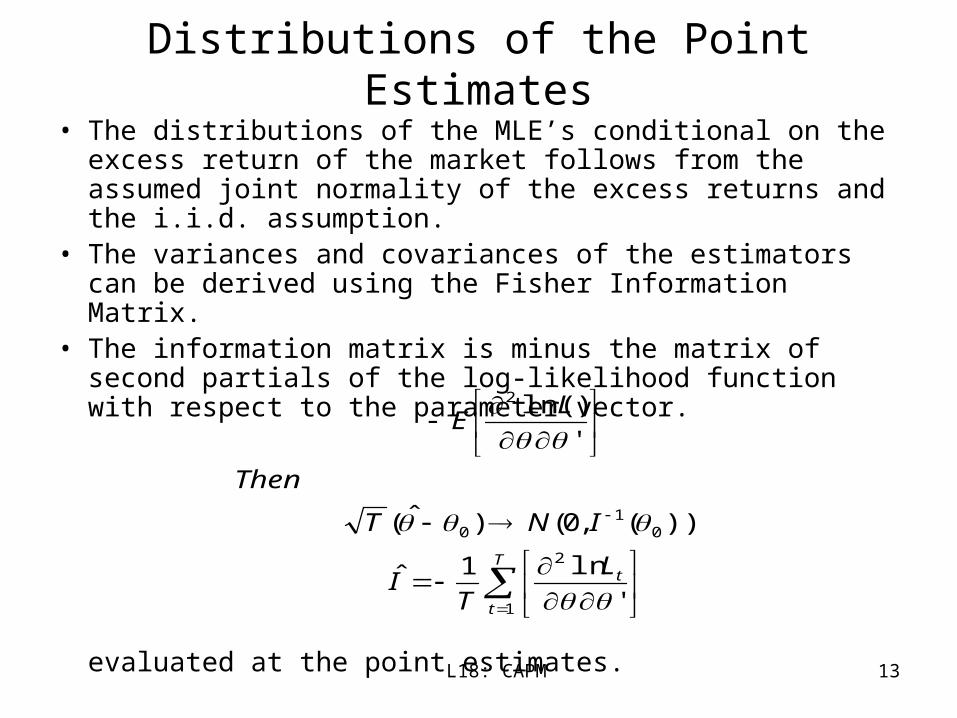
Distributions of the Point Estimates

• The distributions of the MLE’s conditional on the excess return of the market follows from the assumed joint normality of the excess returns and the i.i.d. assumption.

• The variances and covariances of the estimators can be derived using the Fisher Information Matrix.

• The information matrix is minus the matrix of second partials of the log-likelihood function with respect to the parameter vector.

evaluated at the point estimates.

T

t

tL

TI

INT

Then

LE

1

2

01

0

2

'

ln1ˆ

))(,0()ˆ(

'

)ln(

L18: CAPM 14

Asymptotic Properties of Estimators• The estimators are consistent and have the distributions:

• WN(T-2, ) indicates that the NxN covariance matrix T has a Wishart distribution with T-2 degrees of freedom, a multivariate generalization of the chi-squared distribution.

• Note that is independent of both

T

tmmtm

N

m

m

m

ZT

where

TWT

TN

TN

1

22

2

2

2

)ˆ(1

ˆ

),2(~ˆ

ˆ1

11

,~ˆ

ˆ

ˆ1

1,~ˆ

.ˆˆ and

L18: CAPM 15

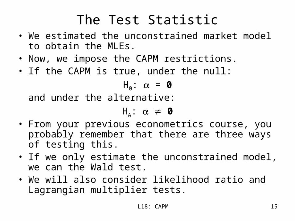
The Test Statistic• We estimated the unconstrained market model to obtain the

MLEs.• Now, we impose the CAPM restrictions.• If the CAPM is true, under the null:

H0: = 0and under the alternative:

HA: 0• From your previous econometrics course, you probably

remember that there are three ways of testing this. • If we only estimate the unconstrained model, we can the Wald

test.• We will also consider likelihood ratio and Lagrangian

multiplier tests.

L18: CAPM 16

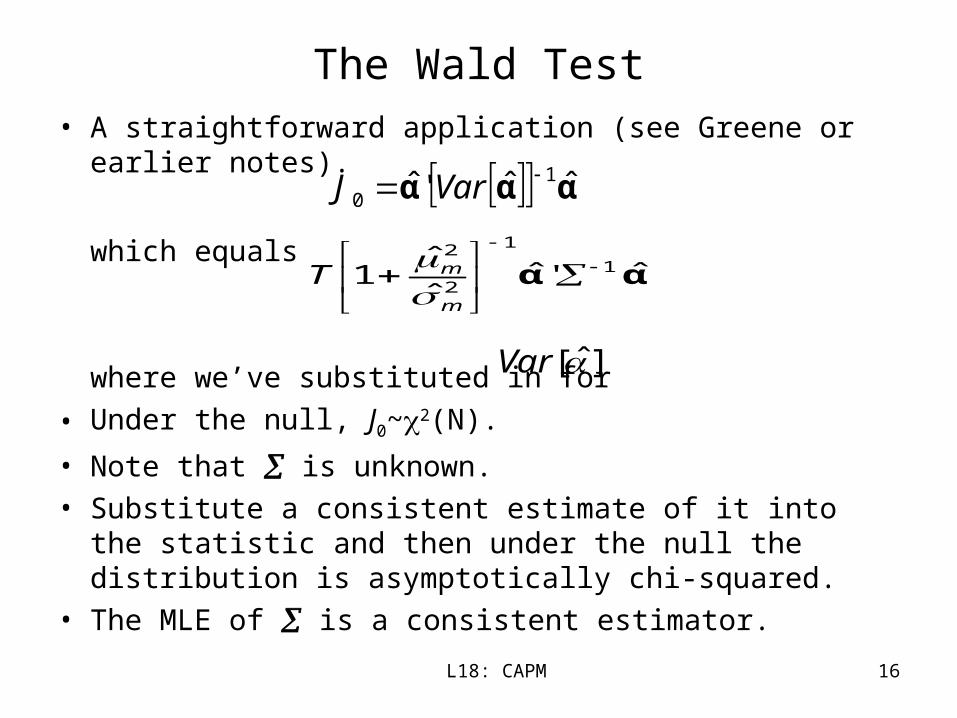
The Wald Test

• A straightforward application (see Greene or earlier notes).

which equals

where we’ve substituted in for

• Under the null, J0~2(N).

• Note that is unknown.

• Substitute a consistent estimate of it into the statistic and then under the null the distribution is asymptotically chi-squared.

• The MLE of is a consistent estimator.

ααα ˆˆ'ˆ 10

VarJ

].ˆ[Var

αα ˆ'ˆˆ

ˆ1 1

1

2

2

m

mT

L18: CAPM 17

We Can Do Better

• The Wald test is an asymptotic test.

• We, however, know the finite sample distribution.

• We can use this to do the Gibbons Ross and Shaken (1989) test.

• To do so, we will need the following theorem from Muirhead (1983).

• Theorem: Let the m-vector x be distributed N(0,), let the (mxm) matrix A be distributed Wm(n,) with nm, and let x and A be independent. Then:

.~')1(

1,

mnmFm

mnxAx 1

L18: CAPM 18

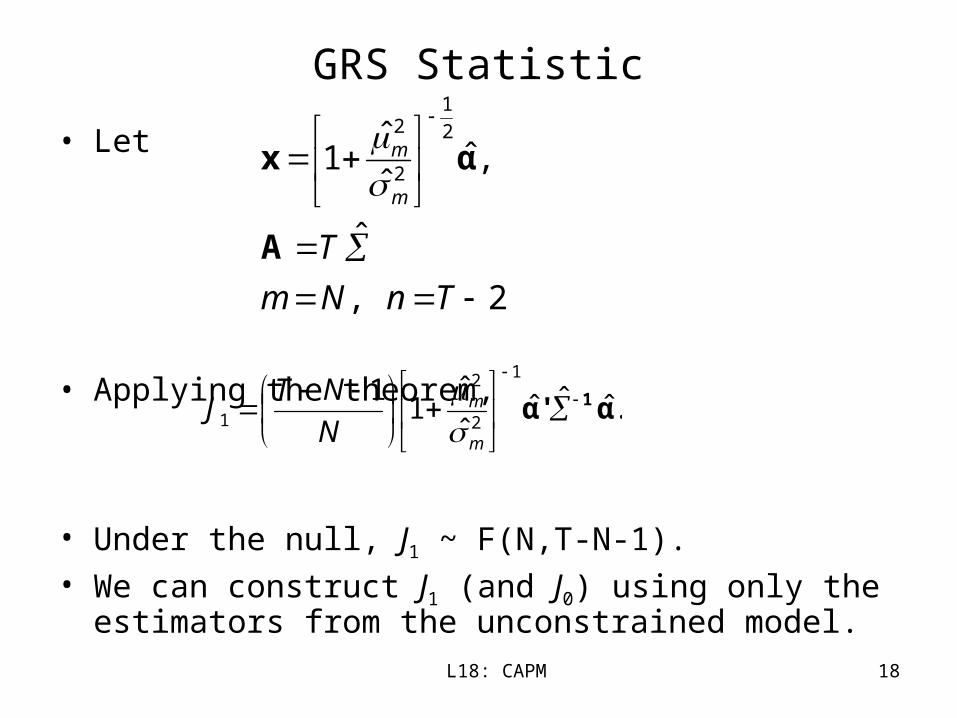
GRS Statistic

• Let

• Applying the theorem,

• Under the null, J1 ~ F(N,T-N-1).• We can construct J1 (and J0) using only the estimators from the

unconstrained model.

2,

ˆ

,ˆˆ

ˆ1

2

1

2

2

TnNm

T

m

m

A

αx

.ˆˆˆˆ

ˆ1

11

2

2

1 α'α 1

m

m

N

NTJ

L18: CAPM 19

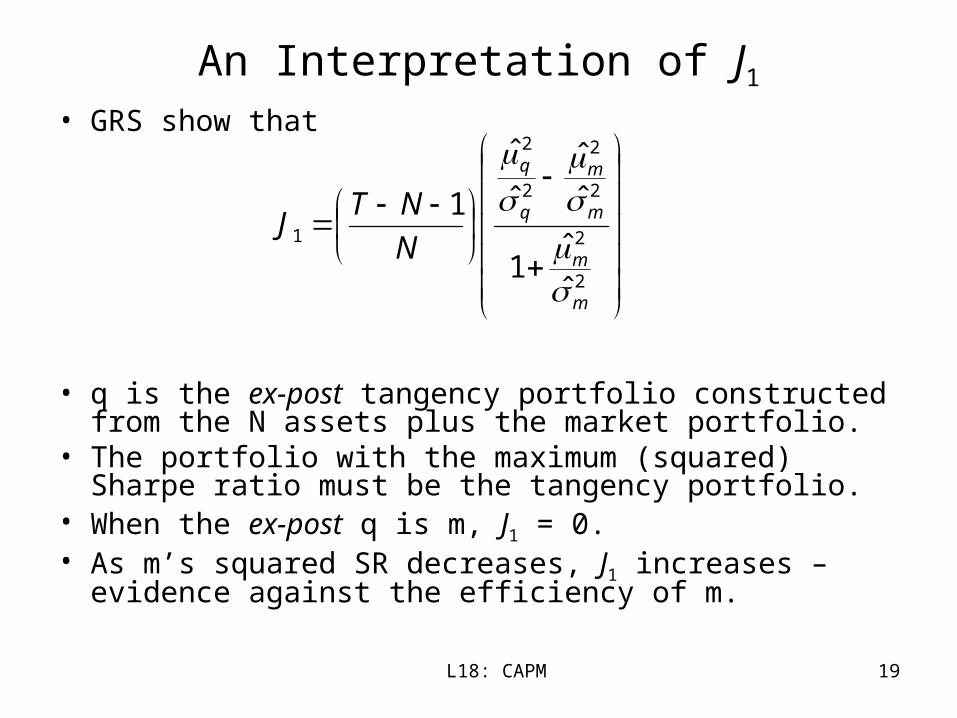
An Interpretation of J1

• GRS show that

• q is the ex-post tangency portfolio constructed from the N assets plus the market portfolio.

• The portfolio with the maximum (squared) Sharpe ratio must be the tangency portfolio.

• When the ex-post q is m, J1 = 0.• As m’s squared SR decreases, J1 increases – evidence against

the efficiency of m.

2

2

2

2

2

2

1

ˆˆ

1

ˆˆ

ˆ

ˆ

1

m

m

m

m

q

q

N

NTJ

L18: CAPM 20

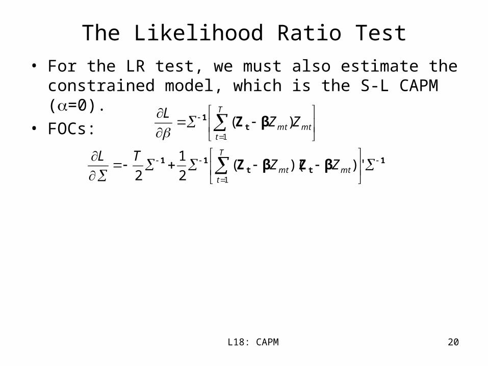
The Likelihood Ratio Test

• For the LR test, we must also estimate the constrained model, which is the S-L CAPM (=0).

• FOCs:

1tt

11

t1

βZβZ

βZ

T

tmtmt

T

tmtmt

ZZTL

ZZL

1

1

)')((2

1

2

)(

L18: CAPM 21

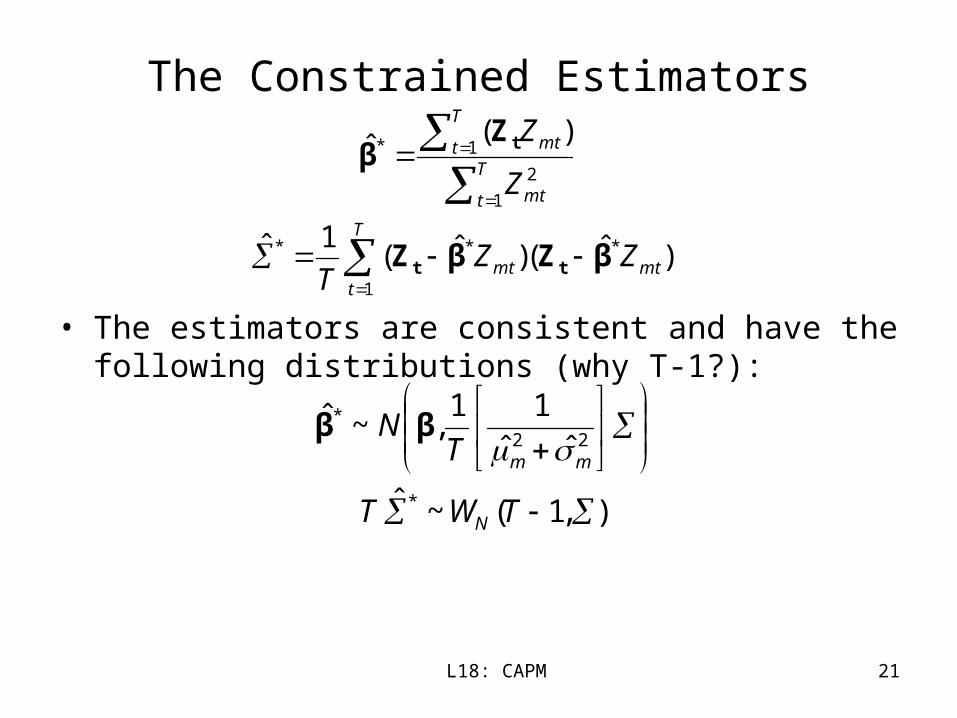
The Constrained Estimators

• The estimators are consistent and have the following distributions (why T-1?):

)'.ˆ()ˆ(1ˆ

)(ˆ

*

1

**

1

2

1*

mt

T

tmt

T

t mt

T

t mt

ZZT

Z

Z

βZβZ

Zβ

tt

t

),1(~ˆ

ˆˆ11

,~ˆ

*

22*

TWT

TN

N

mm ββ

L18: CAPM 22

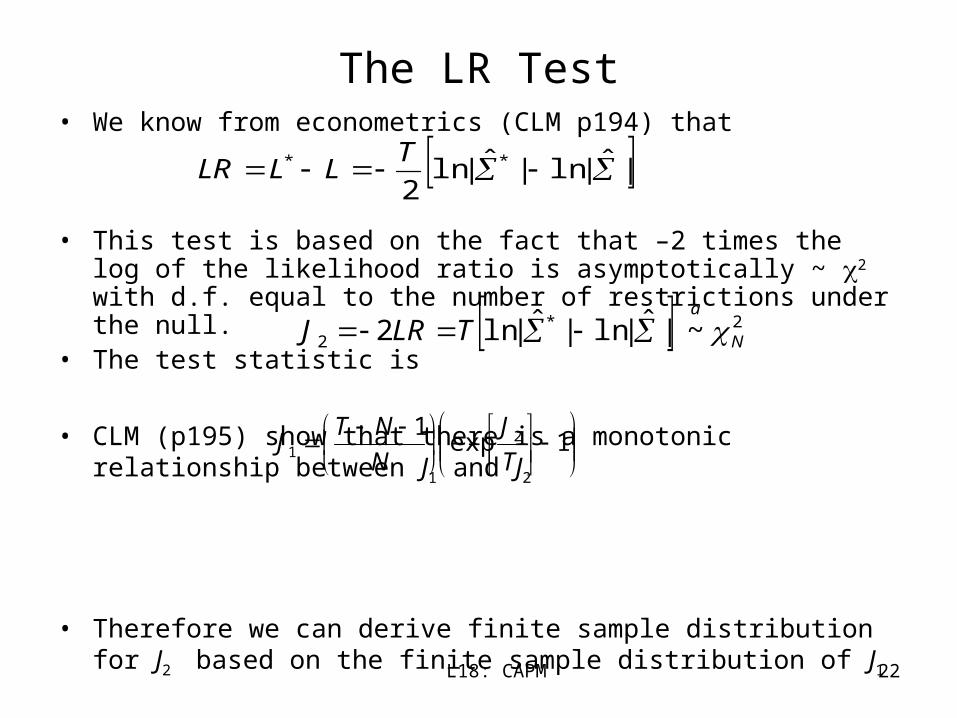
The LR Test• We know from econometrics (CLM p194) that

• This test is based on the fact that –2 times the log of the likelihood ratio is asymptotically ~ 2 with d.f. equal to the number of restrictions under the null.

• The test statistic is

• CLM (p195) show that there is a monotonic relationship between J1 and J2

• Therefore we can derive finite sample distribution for J2 based on the finite sample distribution of J1

|ˆ|ln|ˆ|ln2

** T

LLLR

2*2 ~|ˆ|ln|ˆ|ln2 N

a

TLRJ

1exp1 2

1 T

J

N

NTJ

L18: CAPM 23

Jobson and Korkie (1982) Adjustment

which is also asymptotically distributed as a

• Why do we need different statistics?

• Because although their asymptotic properties are similar, they may have different small-sample properties.

.2N

23

22/J

T

NTaJ

L18: CAPM 24

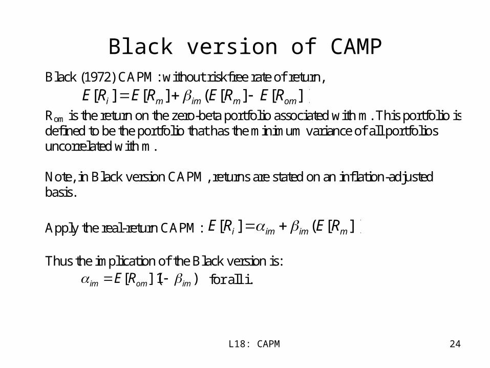
Black version of CAMPBlack (1972) CAPM: without riskfree rate of return,

])[][(][][ ommimmi RERERERE Rom is the return on the zero-beta portfolio associated with m. This portfolio is defined to be the portfolio that has the minimum variance of all portfolios uncorrelated with m. Note, in Black version CAPM, returns are stated on an inflation-adjusted basis.

Apply the real-return CAPM: ])[(][ mimimi RERE Thus the implication of the Black version is: )1]([ imomim RE for all i.

L18: CAPM 25

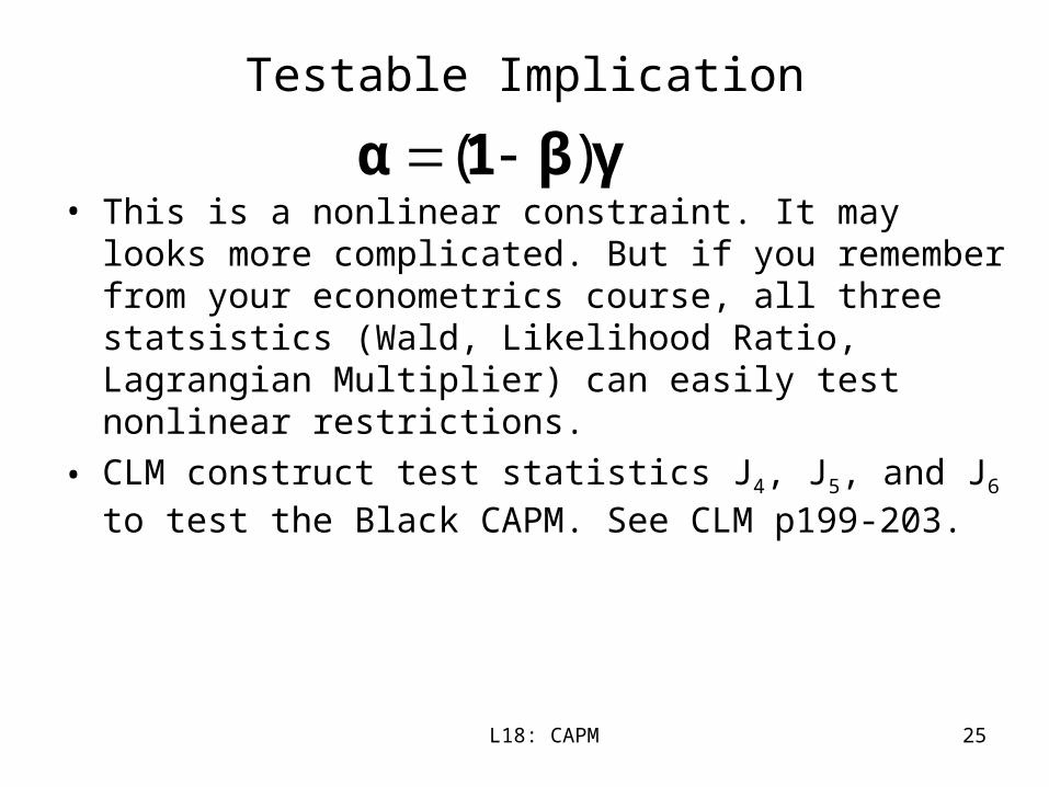
Testable Implication

• This is a nonlinear constraint. It may looks more complicated. But if you remember from your econometrics course, all three statsistics (Wald, Likelihood Ratio, Lagrangian Multiplier) can easily test nonlinear restrictions.

• CLM construct test statistics J4, J5, and J6 to test the Black CAPM. See CLM p199-203.

γβ1α )(

L18: CAPM 26

Size and Power

• They also use simulations to compare small sample properties of all the statistics (Section 5.4 and 5.5 ) – Size simulation: simulate under the null, and compare the

rejection rates under simulation with the theoretical rejection rates

– Power simulation: simulate under the alternative, and see if rejection rate is high enough.

L18: CAPM 27

Further Issues• What if assets returns are not normal?

• One alternative approach is to use quasi-maximum likelihood. Under certain regularity conditions you can estimate the model as if the returns were normally distributed, and the Wald, Likelihood ratio, and Lagrangian multiplier tests are still valid (after adjusting for the covariance matrix for the errors).

• However, small sample properties of QMLE are of serious concern.

• Another alternative is to use GMM, which only rely on a few momentum conditions.

L18: CAPM 28

Cross-sectional Test

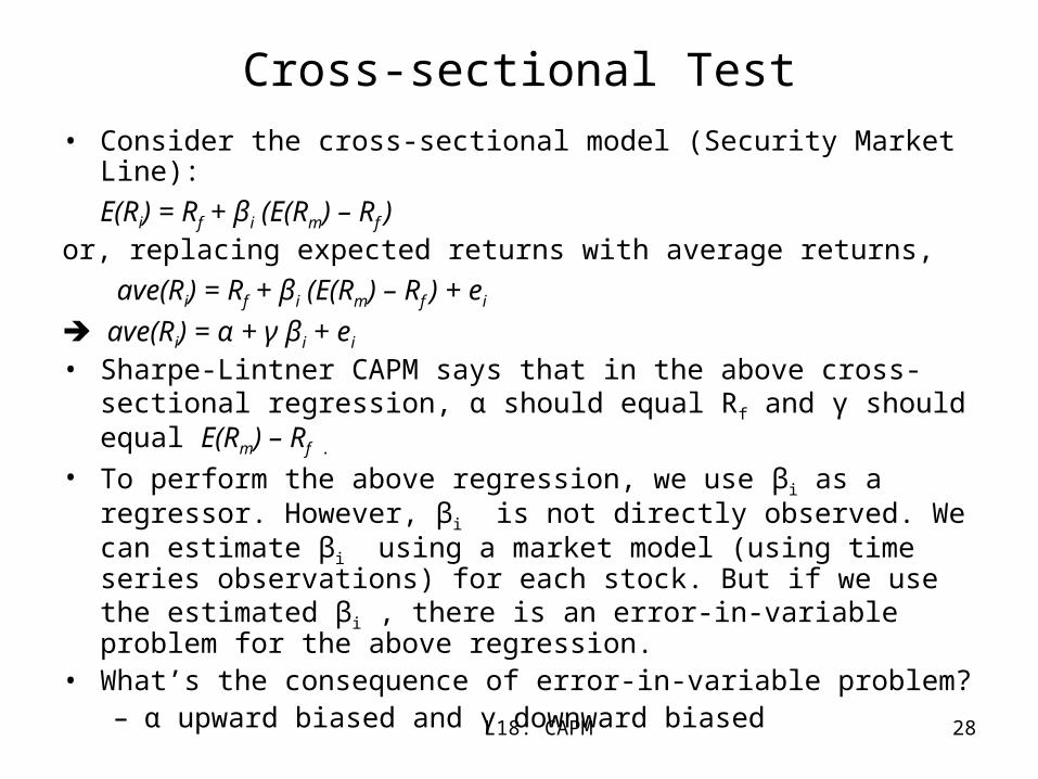
• Consider the cross-sectional model (Security Market Line):

E(Ri) = Rf + βi (E(Rm) – Rf )or, replacing expected returns with average returns,

ave(Ri) = Rf + βi (E(Rm) – Rf ) + ei

ave(Ri) = α + γ βi + ei • Sharpe-Lintner CAPM says that in the above cross-sectional regression, α

should equal Rf and γ should equal E(Rm) – Rf .

• To perform the above regression, we use βi as a regressor. However, βi is not directly observed. We can estimate βi using a market model (using time series observations) for each stock. But if we use the estimated βi , there is an error-in-variable problem for the above regression.

• What’s the consequence of error-in-variable problem?– α upward biased and γ downward biased

L18: CAPM 29

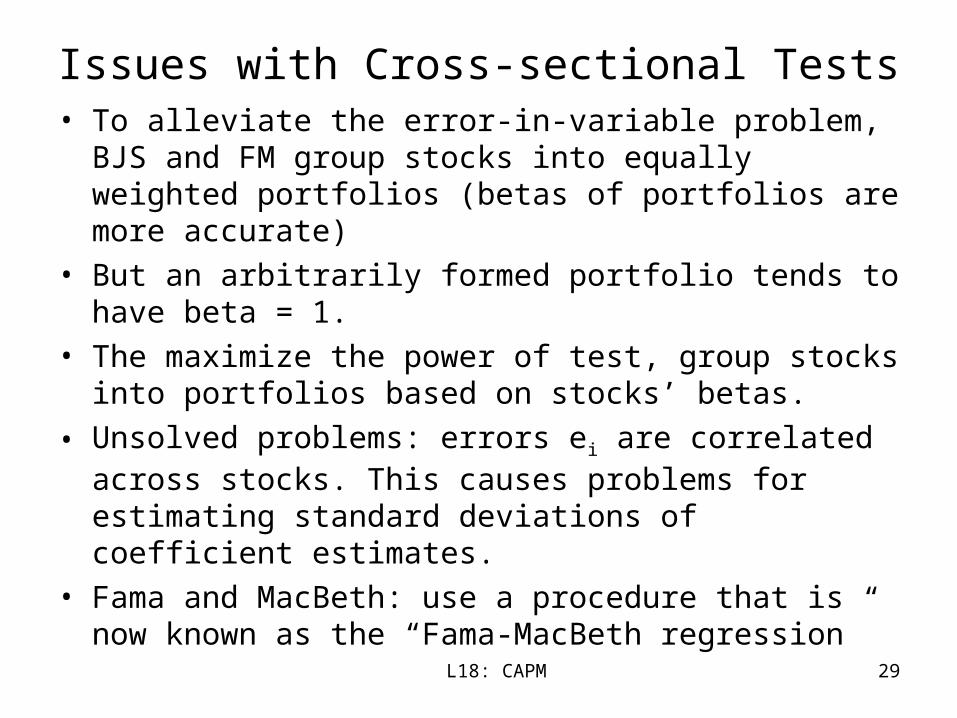
Issues with Cross-sectional Tests• To alleviate the error-in-variable problem, BJS and FM group

stocks into equally weighted portfolios (betas of portfolios are more accurate)

• But an arbitrarily formed portfolio tends to have beta = 1.

• The maximize the power of test, group stocks into portfolios based on stocks’ betas.

• Unsolved problems: errors ei are correlated across stocks. This causes problems for estimating standard deviations of coefficient estimates.

• Fama and MacBeth: use a procedure that is now known as the “Fama-MacBeth regression”

L18: CAPM 30

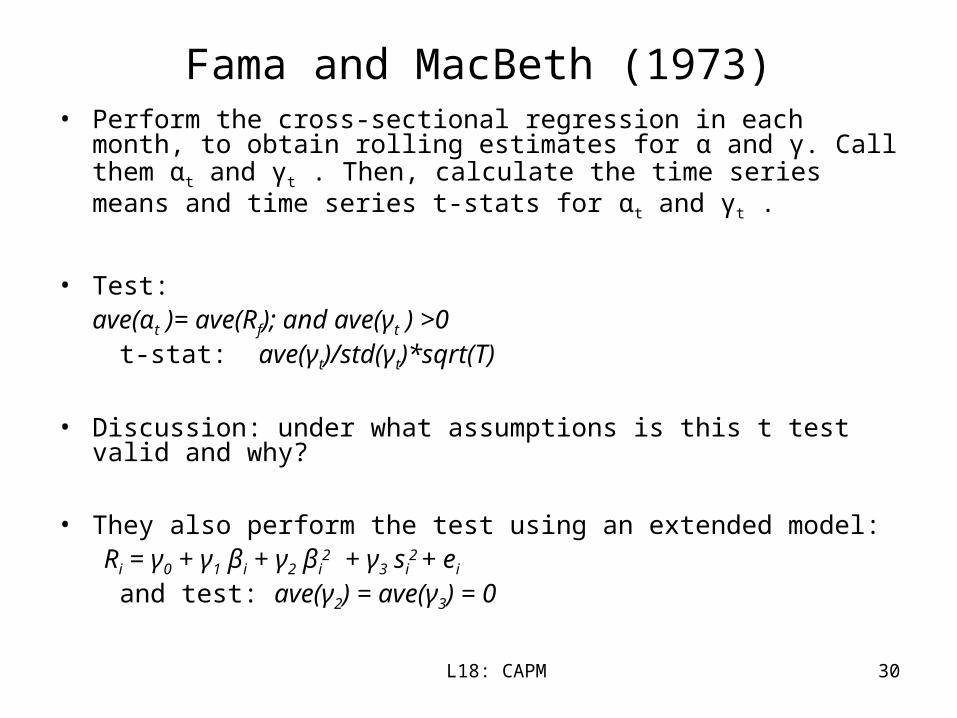
Fama and MacBeth (1973)• Perform the cross-sectional regression in each month, to obtain rolling

estimates for α and γ. Call them αt and γt . Then, calculate the time series means and time series t-stats for αt and γt .

• Test:ave(αt )= ave(Rf); and ave(γt ) >0

t-stat: ave(γt)/std(γt)*sqrt(T)

• Discussion: under what assumptions is this t test valid and why?

• They also perform the test using an extended model: Ri = γ0 + γ1 βi + γ2 βi

2 + γ3 si

2 + ei

and test: ave(γ2) = ave(γ3) = 0

L18: CAPM 31

Results from Cross-sectional Tests

• Estimated α seems too high, relative to the average riskfree rate.

• Estimated γ too low, relative to the average market risk premium.

• Black version of CAPM seems more consistent with the data.

• Other variables, such as squared beta and the variance of idiosyncratic component of returns, do not have marginal power to explain average returns.

• In other words, C1 and C2 seem to hold; C3 is rejected.

L18: CAPM 32

Exercises

• CLM