1

KOZENY-CARMAN EQUATION REVISITED

Jack Dvorkin -- 2009

Abstract

The Kozeny-Carman equation is often presented as permeability versus porosity,

grain size, and tortuosity. When it is used to estimate permeability evolution versus

porosity, some of these arguments (e.g., the grain size and tortuosity) are held constant.

Here we theoretically explore the internal consistency of this assumption and offer

alternative forms for the Kozeny-Carman equation. The only advantage of these forms

over the one traditionally used is their internal consistency. Such analytical solutions

cannot replace measurements, physical and digital, but can rather serve for quality

control of physical and digital data.

1. Problem Formulation

Traditionally, the Kozeny-Carman equation relates the absolute permeability

€

kabsoluteto porosity

€

φ and grain size

€

d as

€

kabsolute ~ d2φ 3 . (1.1)

This form is frequently employed to mimic permeability versus porosity evolution

in datasets, such as in Fontainebleau sandstone (Bourbie and Zinszner, 1985) or Finney

pack (Finney, 1970). During such calculations, the grain size

€

d is typically kept

constant.

We find at least two inconsistencies in this approach: (a) the Kozeny-Carman

equation has been derived for a solid medium with pipe conduits, rather than for a

granular medium and (b) even if a grain size is used in this equation, it is not obvious

that it does not vary with varying porosity (Figure 1.1 and 1.2).

Bearing this argument in mind, we explore how permeability can be predicted

consistently within the Kozeny-Carman formalism, by varying the radii of the conduits,

their number, and type. We find that such a consistent approach is possible. However,

2

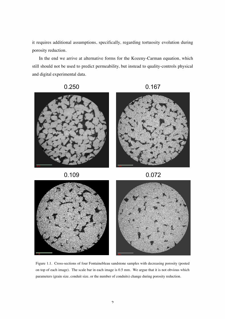
it requires additional assumptions, specifically, regarding tortuosity evolution during

porosity reduction.

In the end we arrive at alternative forms for the Kozeny-Carman equation, which

still should not be used to predict permeability, but instead to quality-controls physical

and digital experimental data.

0.0720.109

0.1670.250

Figure 1.1. Cross-sections of four Fontainebleau sandstone samples with decreasing porosity (posted

on top of each image). The scale bar in each image is 0.5 mm. We argue that it is not obvious which

parameters (grain size, conduit size, or the number of conduits) change during porosity reduction.

3

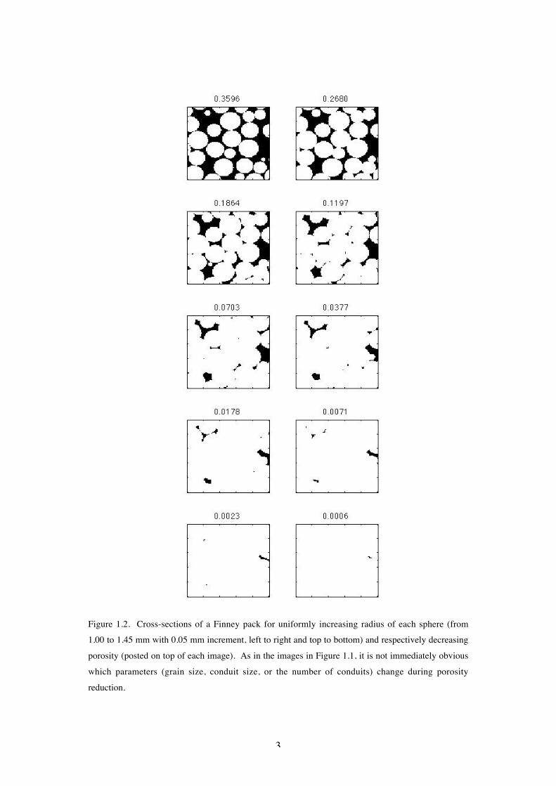
Figure 1.2. Cross-sections of a Finney pack for uniformly increasing radius of each sphere (from

1.00 to 1.45 mm with 0.05 mm increment, left to right and top to bottom) and respectively decreasing

porosity (posted on top of each image). As in the images in Figure 1.1, it is not immediately obvious

which parameters (grain size, conduit size, or the number of conduits) change during porosity

reduction.

4

2. Definition of Absolute Permeability

The definition of absolute permeability

€

kabsolute of porous rock comes from Darcy’s

equation (e.g., Mavko et al., 1998)

€

Q = −kabsoluteAµdPdx, (2.1)

where

€

Q is the volume flux through the sample (in, e.g., m3/s);

€

A is the cross-sectional

area of the sample (in, e.g., m2);

€

µ is the dynamic viscosity of the fluid (in, e.g., Pa s

with 1 cPs = 10-3 Pa s); and

€

dP /dx is the pressure drop across the sample divided by the

length of the sample (in, e.g., Pa/m).

3. Flow Through a Circular Pipe

The equation for laminar viscous flow in a pipe of radius

€

b is

€

∂ 2u∂r2

+1r∂u∂r

=1µdPdx, (3.1)

where

€

u is the velocity of the fluid in the axial (

€

x) direction;

€

µ is the dynamic viscosity

of the fluid;

€

dP /dx is the pressure gradient in the axial direction; and

€

r and

€

x are the

radial and axial coordinates, respectively.

A general solution of Equation (3.1) is

€

u = ˜ A + ˜ B r2 + ˜ C ln r, (3.2)

where

€

˜ A ,

€

˜ B , and

€

˜ C are constants. It follows from Equation (3.2) that

€

∂u∂r

= 2 ˜ C r +˜ C r

, ∂ 2u∂r2 = 2 ˜ C −

˜ C r2 . (3.3)

By substituting the expressions from Equation (3.3) into Equation (3.1) we find that

€

2 ˜ B −˜ C

r2 + 2 ˜ B +˜ C

r2 =1µ

dPdy

, (3.4)

which means that

€

˜ B = 14µ

dPdx

. (3.5)

5

To avoid singularity at

€

r = 0 we need to assume that in Equation (3.2)

€

˜ C = 0.

Next, we will employ the no-slip condition

€

u = 0 at

€

r =

€

b.

€

u = ˜ A + ˜ B r2 = ˜ A + 14µ

dPdx

r2 = ˜ A + 14µ

dPdx

b2 = 0, (3.6)

which means

€

˜ A = − 14µ

dPdx

b2 (3.7)

and

€

u = −14µ

dPdx

b2(1− r2

b2). (3.8)

The total volume flux through the pipe is

€

q = −πb4

8µΔPl, (3.9)

where

€

l is the length of the pipe,

€

ΔP is the pressure head along the length of the pipe,

and the pressure gradient

€

dP /dx is replaced with

€

ΔP / l .

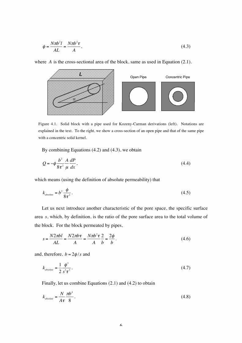
4. Absolute Permeability – Round Pipe

Assume that a pore space is made of

€

N identical parallel round pipes embedded in a

solid block at an angle

€

α to its horizontal face (Figure 4.1). The horizontal pressure

head across the block is

€

ΔP . The length of each pipe inside the block is

€

l = L /sinα = Lτ, (4.1)

where

€

L is the horizontal length of the block and, by definition,

€

τ = sin−1α is the

tortuosity.

Using Equations (3.9) and (4.1), we obtain the total flux through

€

N pipes as

€

Q = Nq = −N πb4

8µΔPLτ

= −N πb4

8µτdPdx

= −Nπb2τ b2

8µτ 2dPdx, (4.2)

where

€

ΔP /Lτ is the pressure gradient across the pipe.

The porosity of the block due to the pipes is

6

€

φ =Nπb2lAL

=Nπb2τA

, (4.3)

where

€

A is the cross-sectional area of the block, same as used in Equation (2.1).

Figure 4.1. Solid block with a pipe used for Kozeny-Carman derivations (left). Notations are

explained in the text. To the right, we show a cross-section of an open pipe and that of the same pipe

with a concentric solid kernel.

By combining Equations (4.2) and (4.3), we obtain

€

Q = −φb2

8τ 2AµdPdx, (4.4)

which means (using the definition of absolute permeability) that

€

kabsolute = b2 φ8τ 2

. (4.5)

Let us next introduce another characteristic of the pore space, the specific surface

area

€

s, which, by definition, is the ratio of the pore surface area to the total volume of

the block. For the block permeated by pipes,

€

s =N2πblAL

=N2πbτA

=Nπb2τA

2b

=2φb. (4.6)

and, therefore,

€

b = 2φ /s and

€

kabsolute =12φ 3

s2τ 2. (4.7)

Finally, let us combine Equations (2.1) and (4.2) to obtain

€

kabsolute =NAτ

πb4

8. (4.8)

7

5. Absolute Permeability -- Concentric Pipe

Consider fluid flow through a round pipe of radius

€

b with a concentric solid kernel

of radius

€

a inside (Figure 4.1). Equations (3.1) and (3.2) are still valid for the flow

inside the annular gap formed by the pipe and kernel. The solution for velocity

€

u inside

the annular gap is obtained from Equation (3.2) and using the no-slip (

€

u = 0) boundary

conditions at

€

r =

€

b and

€

r =

€

a :

€

u = −14µ

dPdx

b2[(1− r2

b2) − (1− a

2

b2) ln(b /r)ln(b /a)

]. (5.1)

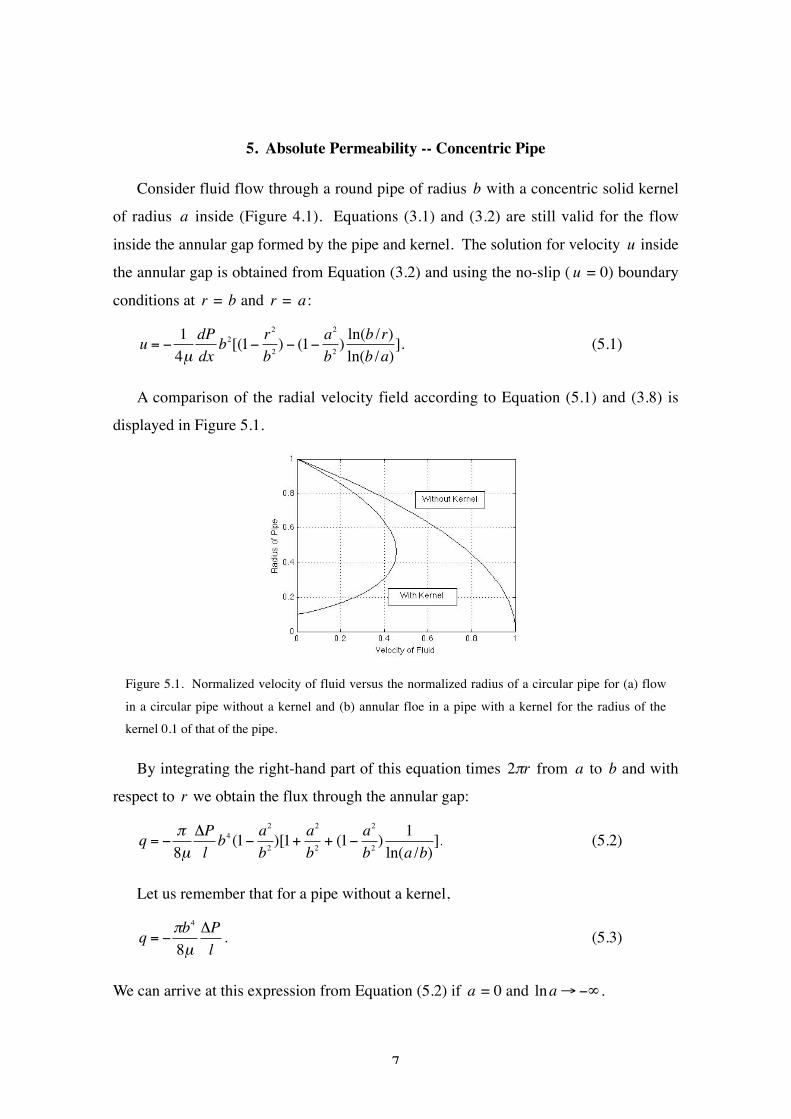
A comparison of the radial velocity field according to Equation (5.1) and (3.8) is

displayed in Figure 5.1.

Figure 5.1. Normalized velocity of fluid versus the normalized radius of a circular pipe for (a) flow

in a circular pipe without a kernel and (b) annular floe in a pipe with a kernel for the radius of the

kernel 0.1 of that of the pipe.

By integrating the right-hand part of this equation times

€

2πr from

€

a to

€

b and with

respect to

€

r we obtain the flux through the annular gap:

€

q = −π8µ

ΔPlb4 (1− a

2

b2)[1+

a2

b2+ (1− a

2

b2) 1ln(a /b)

]. (5.2)

Let us remember that for a pipe without a kernel,

€

q = −πb4

8µΔPl. (5.3)

We can arrive at this expression from Equation (5.2) if

€

a = 0 and

€

lna→−∞ .

8

Also, if

€

a→ b, the infinity in the denominator of the third term in the square

brackets in Equation (5.2) has the same order as that in the numerator, and

€

q→ 0 .

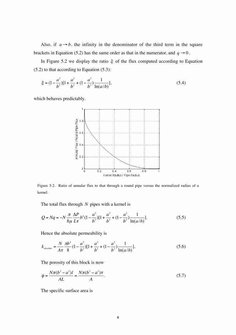
In Figure 5.2 we display the ratio

€

ξ of the flux computed according to Equation

(5.2) to that according to Equation (5.3):

€

ξ = (1− a2

b2)[1+

a2

b2+ (1− a

2

b2) 1ln(a /b)

], (5.4)

which behaves predictably.

Figure 5.2. Ratio of annular flux to that through a round pipe versus the normalized radius of a

kernel.

The total flux through

€

N pipes with a kernel is

€

Q = Nq = −N π8µ

ΔPLτ

b4 (1− a2

b2)[1+

a2

b2+ (1− a

2

b2) 1ln(a /b)

]. (5.5)

Hence the absolute permeability is

€

kabsolute =NAτ

πb4

8(1− a

2

b2)[1+

a2

b2+ (1− a

2

b2) 1ln(a /b)

]. (5.6)

The porosity of this block is now

€

φ =Nπ (b2 − a2)l

AL=Nπ (b2 − a2)τ

A. (5.7)

The specific surface area is

9

€

s =N2π (b + a)l

AL=N2π (b + a)τ

A=Nπ (b2 − a2)τ

A2

b − a=2φb − a

. (5.8)

As a result,

€

kabsolute =φ8τ 2

b2[1+a2

b2+ (1− a

2

b2) 1ln(a /b)

]. (5.9)

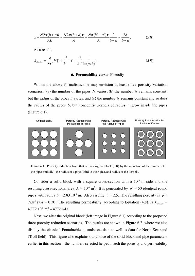
6. Permeability versus Porosity

Within the above formalism, one may envision at least three porosity variation

scenarios: (a) the number of the pipes

€

N varies, (b) the number

€

N remains constant,

but the radius of the pipes

€

b varies, and (c) the number

€

N remains constant and so does

the radius of the pipes

€

b, but concentric kernels of radius

€

a grow inside the pipes

(Figure 6.1).

Original Block Porosity Reduces withthe Number of Pipes

Porosity Reduces withthe Radius of Pipes

Porosity Reduces with theRadius of Kernels

Figure 6.1. Porosity reduction from that of the original block (left) by the reduction of the number of

the pipes (middle), the radius of a pipe (third to the right), and radius of the kernels.

Consider a solid block with a square cross-section with a 10-3 m side and the

resulting cross-sectional area

€

A = 10-6 m2. It is penetrated by

€

N = 50 identical round

pipes with radius

€

b = 2.83·10-5 m. Also assume

€

τ = 2.5. The resulting porosity is

€

φ =

€

Nπb2τ /A = 0.30. The resulting permeability, according to Equation (4.8), is

€

kabsolute =

4.772·10-5 m2 = 4772 mD.

Next, we alter the original block (left image in Figure 6.1) according to the proposed

three porosity reduction scenarios. The results are shown in Figure 6.2, where we also

display the classical Fontainebleau sandstone data as well as data for North Sea sand

(Troll field). This figure also explains our choice of the solid block and pipe parameters

earlier in this section – the numbers selected helped match the porosity and permeability

10

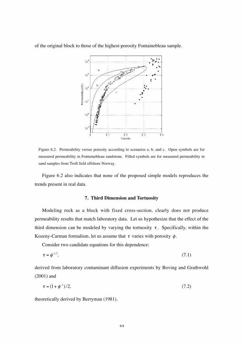
of the original block to those of the highest-porosity Fontainebleau sample.

Figure 6.2. Permeability versus porosity according to scenarios a, b, and c. Open symbols are for

measured permeability in Fontainebleau sandstone. Filled symbols are for measured permeability in

sand samples from Troll field offshore Norway.

Figure 6.2 also indicates that none of the proposed simple models reproduces the

trends present in real data.

7. Third Dimension and Tortuosity

Modeling rock as a block with fixed cross-section, clearly does not produce

permeability results that match laboratory data. Let us hypothesize that the effect of the

third dimension can be modeled by varying the tortuosity

€

τ . Specifically, within the

Kozeny-Carman formalism, let us assume that

€

τ varies with porosity

€

φ .

Consider two candidate equations for this dependence:

€

τ = φ−1.2, (7.1)

derived from laboratory contaminant diffusion experiments by Boving and Grathwohl

(2001) and

€

τ = (1+ φ−1) /2, (7.2)

theoretically derived by Berryman (1981).

11

At

€

φ = 0.3, these two equations give

€

τ = 4.24 and 2.17, respectively.

Let us next repeat out calculations of permeability for the three porosity evolution

scenarios, but this time with the tortuosity varying versus porosity. Also, to keep the

scale consistent, we will scale Equations (7.1) and (7.2) to yield

€

τ = 2.5 at

€

φ = 0.3 as

follows

€

τ = 0.590φ−1.2 (7.3)

and

€

τ = 0.576(1+ φ−1). (7.4)

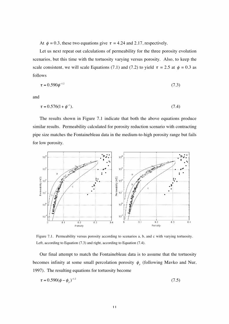
The results shown in Figure 7.1 indicate that both the above equations produce

similar results. Permeability calculated for porosity reduction scenario with contracting

pipe size matches the Fontainebleau data in the medium-to-high porosity range but fails

for low porosity.

Figure 7.1. Permeability versus porosity according to scenarios a, b, and c with varying tortuosity.

Left, according to Equation (7.3) and right, according to Equation (7.4).

Our final attempt to match the Fontainebleau data is to assume that the tortuosity

becomes infinity at some small percolation porosity

€

φ p (following Mavko and Nur,

1997). The resulting equations for tortuosity become

€

τ = 0.590(φ − φ p )−1.2 (7.5)

12

and

€

τ = 0.576[1+ (φ − φ p )−1]. (7.6)

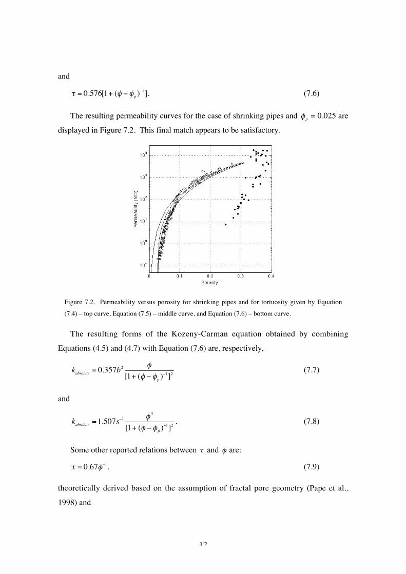
The resulting permeability curves for the case of shrinking pipes and

€

φ p = 0.025 are

displayed in Figure 7.2. This final match appears to be satisfactory.

Figure 7.2. Permeability versus porosity for shrinking pipes and for tortuosity given by Equation

(7.4) – top curve, Equation (7.5) – middle curve, and Equation (7.6) – bottom curve.

The resulting forms of the Kozeny-Carman equation obtained by combining

Equations (4.5) and (4.7) with Equation (7.6) are, respectively,

€

kabsolute = 0.357b2 φ[1+ (φ − φ p )

−1]2(7.7)

and

€

kabsolute =1.507s−2 φ 3

[1+ (φ − φ p )−1]2. (7.8)

Some other reported relations between

€

τ and

€

φ are:

€

τ = 0.67φ−1, (7.9)

theoretically derived based on the assumption of fractal pore geometry (Pape et al.,

1998) and

13

€

τ =1.8561− 0.715φ, 0.1< φ < 0.5;τ = 2.1445 −1.126φ, 0.3 < φ < 0.5;τ = −2.1472 + 5.244φ, 0.6 < φ <1.0;

(7.10)

derived from laboratory fluid flow experiments on textiles, kaolinite, and soil by Salem

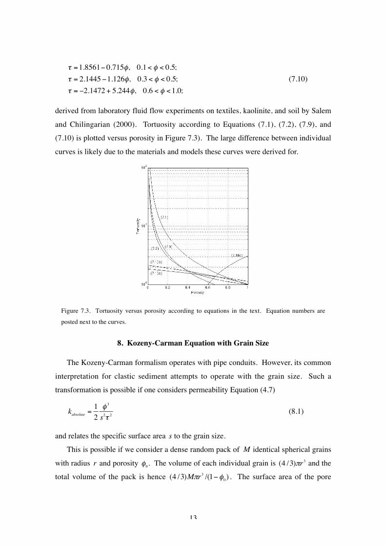
and Chilingarian (2000). Tortuosity according to Equations (7.1), (7.2), (7.9), and

(7.10) is plotted versus porosity in Figure 7.3). The large difference between individual

curves is likely due to the materials and models these curves were derived for.

Figure 7.3. Tortuosity versus porosity according to equations in the text. Equation numbers are

posted next to the curves.

8. Kozeny-Carman Equation with Grain Size

The Kozeny-Carman formalism operates with pipe conduits. However, its common

interpretation for clastic sediment attempts to operate with the grain size. Such a

transformation is possible if one considers permeability Equation (4.7)

€

kabsolute =12φ 3

s2τ 2(8.1)

and relates the specific surface area

€

s to the grain size.

This is possible if we consider a dense random pack of

€

M identical spherical grains

with radius

€

r and porosity

€

φ0. The volume of each individual grain is

€

(4 /3)πr3 and the

total volume of the pack is hence

€

(4 /3)Mπr3 /(1−φ0) . The surface area of the pore

14

space is

€

4Mπr2. Therefore, for this specific case,

€

s = 3(1−φ0) /r = 6(1−φ0) /d, (8.2)

where

€

d = 2

€

r .

Note that this equation is only valid for a sphere pack with porosity

€

φ0 ≈ 0.36. If

we assume that the same equation applies to the entire porosity range, which is clearly

invalid since

€

s should be generally decreasing with decreasing porosity, we obtain form

Equations (8.1) and (8.2)

€

kabsolute =r2

18φ 3

(1−φ)2τ 2=d 2

72φ 3

(1−φ)2τ 2, (8.3)

where

€

d = 2

€

r .

We can also modify this last equation by introducing a percolation porosity

€

φ p

(Mavko and Nur, 1997) as

€

kabsolute =d 2

72(φ − φ p )

3

(1−φ + φ p )2τ 2, (8.4)

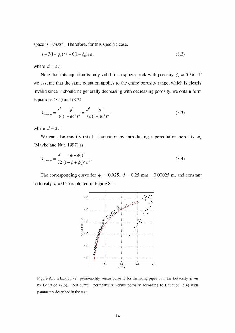
The corresponding curve for

€

φ p = 0.025,

€

d = 0.25 mm = 0.00025 m, and constant

tortuosity

€

τ = 0.25 is plotted in Figure 8.1.

Figure 8.1. Black curve: permeability versus porosity for shrinking pipes with the tortuosity given

by Equation (7.6). Red curve: permeability versus porosity according to Equation (8.4) with

parameters described in the text.

15

9. Conclusion

Consistency is possible in deriving and applying Kozeny-Carman equation for

permeability as a function of porosity. Any such derivation inherently requires such

idealized and, generally, nonexistent in real rock parameters as grain size, pore size, and

tortuosity. Yet, the Kozeny-Carman equation can be made to mimic some experimental

trends and, therefore, serve as a quality-control tool for physical and digital

experimental results.

References

Berryman, J.G., 1981, Elastic wave propagation in fluid-saturated porous media,

Journal of Acoustical Society of America, 69, 416-424.

Bourbie, T., and Zinszner, B., 1985, Hydraulic and acoustic properties as a function of

porosity in Fontainebleau Sandstone, Journal of Geophysical Research, 90, 11,524-

11,532.

Boving, T.B., and Grathwohl, P., 2001, Tracer diffusion coefficients in sedimentary

rocks: correlation to porosity and hydraulic conductivity, Journal of Contaminant

Hydrology, 53, 85-100.

Finney, J., 1970, Random packing and the structure of simple liquids (The geometry of

random close packing), Proceedings of the Royal Society, 319A, 479.

Mavko, G., and Nur, A., 1997, The effect of a percolation threshold in the Kozeny-

Carman relation, Geophysics, 62, 1480-1482.

Pape, H., Clauser, C., and Iffland, J., 1998, Permeability prediction for reservoir

sandstones and basement rocks based on fractal pore space geometry, SEG

Expanded Abstracts, SEG 1998 Meeting.

Salem, H., and Chilingarian, G.V., 2000, Influence of porosity and direction of flow on

tortuosity in unconsolidated porous media, Energy Sources, 22, 207-213.

16

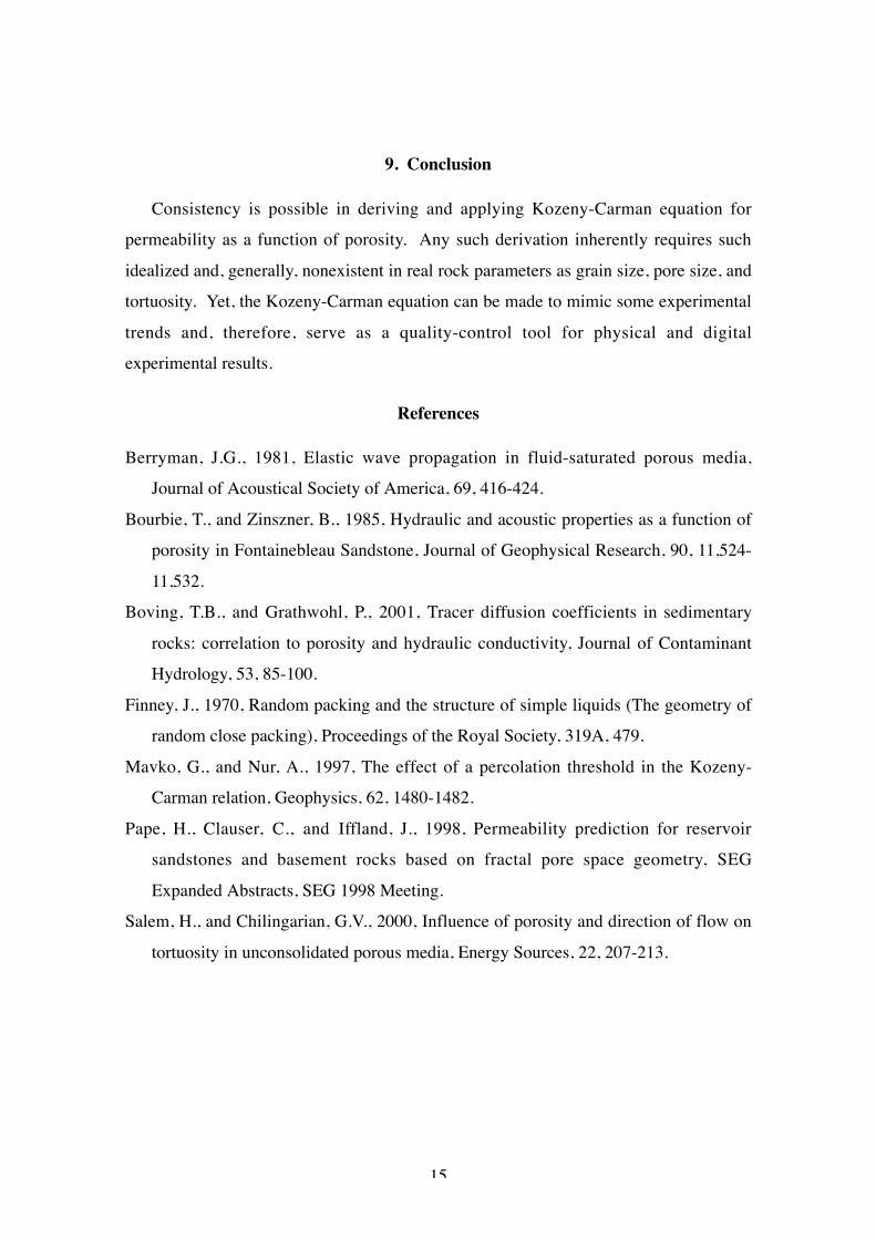
Appendix: Specific Surface Area of the Finney Pack with Expanding Spheres

We select a cubic subset of the Finney pack and gradually and uniformly expand the

radius of each sphere from 1 to 1.5 mm. The evolution of the porosity of these packs

versus the radius of a sphere is shown in Figure A.1.

Figure A.1. Left – porosity of a Finney pack decreasing with the increasing radius of each sphere.

Middle – the specific surface area decreasing with the increasing radius of each sphere. Right – the

specific surface area increasing with increasing porosity (black). The red curve is computed from

Equation (A.1) with fixed sphere radius 1 mm. The blue curve is also computed from Equation (A.1)

but with respectively increasing sphere radius.

In the same figure we display the calculated specific surface area versus the radius

and the specific surface area versus the porosity. In the latter frame, we also display a

theoretical curve according to equation

€

s = 3(1−φ) /r (A.1)

for varying porosity and fixed radius

€

r = 1 and for varying porosity and varying radius.

Neither of these two theoretical curves even qualitatively matches the computed specific

surface area.